The relationship between hydrodynamic variables
and particle size distribution in flotation
Thèse
Ali Vazirizadeh
Doctorat en génie des matériaux et de la métallurgie
Philosophiæ Doctor (Ph.D.)
Québec, Canada
iii
Résumé
La flottation industrielle est un procédé continu qui se déroule souvent en plusieurs étapes et dans lequel des particules d'une espèce de minéral donnée (généralement celles d'intérêt), présentes en différentes tailles, rencontrent une grande quantité de bulles de gaz (normalement de l'air) pour produire des agrégats bulles-particules minérales, qui sont extraits du dispositif de flottation (colonne ou cellule) en tant que produit de valeur (concentré). Le contenu en bulles est décrit par les conditions hydrodynamiques régnant dans le réacteur de flottation. Celles-ci sont reconnues pour leur influence sur la performance de la flottation.
Ce projet de recherche porte sur deux sujets majeurs. Le premier est l'analyse de l’impact des particules solides sur les variables hydrodynamiques et l’effet de ces variables hydrodynamiques sur la récupération d’eau au concentré. Pour ce faire, l'effet du solide sur la distribution de la taille des bulles et le taux de rétention de l’air, ainsi que la corrélation entre la distribution de taille des bulles et le taux de rétention de l’air dans une colonne de flottation ont été étudiés. L'effet du taux de rétention de l’air, de la dimension des bulles et du taux surfacique de bulles (Sb) sur la quantité d’eau extraite au concentré a ensuite été
analysé.
Le second sujet traite de l'utilisation des variables hydrodynamiques pour la modélisation de la cinétique du procédé de flottation selon distribution granulométrique des particules introduites. La surface inter-faciale de bulle (Ib) est introduite à cet égard comme une
variable hydrodynamique fournissant plus d'informations sur la distribution de taille de bulle que le taux surfacique de bulles qui est plus couramment utilisé. De plus, la corrélation entre la constante cinétique, la taille des particules et certaines variables hydrodynamiques a été analysée en utilisant une projection de structures latentes (PSL). Les résultats indiquent que l'importance relative des variables hydrodynamiques pour la modélisation de la cinétique de flottation dépend de la distribution granulométrique des particules. Finalement, les variables hydrodynamiques suggérées pour chaque classe granulométrique considérée ont été utilisées pour produire des modèles de régression mono-variable de la constante cinétique.
v
Abstract
Industrial flotation is a continuous and often multistage process, where particles of a given mineral species (usually the targeted one), present in different sizes, encounter a large amount of gas bubbles (normally air) to produce mineral–bubble aggregates, which are removed from the flotation device (cell or column) as a valuable product (concentrate). The bubble content inside the cell is characterized by the prevailing hydrodynamic conditions (known as gas dispersion variables), which in turn are known to influence the flotation performance.
This research project deals with two major topics. The first one is identifying the effect of mineral particles on hydrodynamic variables, and the effects of hydrodynamic variables on the final water recovery. For this purpose, the effect of solid particles on the bubble size distribution and gas hold-up, as well as the correlation between bubble size distribution and gas hold-up in column flotation were studied. It is followed by an assessment of the effect of the gas hold-up, bubble size and bubble surface area flux (Sb) on the amount of water
reporting to the concentrate.
The second topic deals with applying appropriate hydrodynamic variables for flotation modeling based on a given introduced particle size distribution. The interfacial area of bubbles (Ib) is introduced to address this issue as a hydrodynamic variable providing more
information about the size distribution of bubbles than the commonly used bubble surface area flux. The correlation between the flotation rate constant and particle size as well as given hydrodynamic variables using a Projection to Latent Structures (PLS) has been analyzed. Results suggest that the relative importance of hydrodynamic variables for flotation rate modeling depends on the particle size distribution. Finally the suggested hydrodynamic variables for each of the various particle size-classes considered were used to produce single variable models for the flotation rate constant.
vii
Table of contents
Résumé ... iii
Abstract ... v
List of Tables ... xi
List of Figures ... xiii
Nomenclature ... xvii
Acknowledgments ... xxi
Foreword ... xxiii
Chapter 1 Introduction ... 1
1.1 Principles of flotation ... 1
1.2 Hydrophobic and hydrophilic particles ... 1
1.3 Use of reagents in flotation practice ... 2
1.3.1 Collectors ... 2 1.3.2 Modifiers ... 3 1.3.3 Frothers ... 3 1.4 Bubble-particle collection ... 4 1.4.1 Bubble-Particle Collision ... 5 1.4.2 Particle attachment ... 7 1.4.3 Particle detachment ... 8 1.4.4 Particle entrainment ... 9 1.5 Flotation devices ... 10 1.5.1 Mechanical cells ... 10 1.5.2 Flotation columns ... 11 1.6 Flotation modeling ... 15 1.6.1 Performance justification ... 15
1.6.2 Kinetic constant modeling ... 18
1.6.3 Residence time measurement in a flotation column ... 21
1.7 Gas dispersion properties ... 22
1.7.1 Gas hold-up (εg) ... 22
viii
1.7.3 Bubble surface area flux (Sb) ... 23
1.7.4 Bubble size distribution ... 26
1.7.5 Gas dispersion properties range and effects ... 27
1.8 Relation between the kinetic constant and gas dispersion properties ... 29
1.9 Problems associated to the use of a single Sb value... 30
1.10 Assumptions made in this experimental work... 33
1.10.1 Hydrophobicity ... 33
1.10.2 Solid particle residence time ... 33
1.10.3 Ultimate recovery (R∞) ... 34
1.10.4 Froth depth and its effect on the final recovery ... 35
1.11 Experimental set-up and results... 35
1.12 Objectives ... 36
1.13 Outline of the thesis ... 37
Chapter 2 Effect of particles on the bubble size distribution and gas hold-up in column flotation ... 41
2.1 Introduction ... 42
2.2 Experimental set-up ... 43
2.3 Results and discussion ... 48
2.3.1 Solid particles on the bubble size distribution ... 48
2.3.2 Effect of solid particles on the gas hold-up ... 55
2.3.3 Discussion ... 59
2.4 Conclusion ... 61
Chapter 3 The effect of gas dispersion properties on water recovery in a laboratory flotation column ... 63
3.1 Introduction ... 64
3.2 Results and discussion ... 66
3.2.1 Effect of gas dispersion properties on the water recovery ... 66
3.2.2 Effect of hydrophobic particle size on the water recovery ... 69
3.2.3 Effect of gas dispersion properties on the carrying capacity ... 70
ix Chapter 4 On the relationship between hydrodynamic characteristics and the kinetics of
column flotation. Part I: modeling the gas dispersion ... 73
4.1 Introduction ... 74
4.1.1 Hydrodynamic variables and particle size ... 75
4.1.2 Bubble surface area flux models ... 76
4.1.3 Bubble size measurement ... 77
4.1.4 Bubble size distribution ... 78
4.2 Equations of gas dispersion... 80
4.2.1 Normal distribution ... 80
4.2.2 Log-normal distribution ... 82
4.3 Test procedure ... 84
4.4 Results and discussion ... 85
4.4.1 Modeling the experimental bubble size distributions ... 85
4.4.2 Correlations between hydrodynamic variables ... 88
4.5 Conclusion ... 92
Chapter 5 On the relationship between hydrodynamic characteristics and the kinetics of flotation. Part II: model validation ... 95
5.1 Introduction ... 96
5.2 Test procedure ... 99
5.3 Results and discussion ... 100
5.3.1 Particle size and kinetic constants ... 100
5.3.2 Hydrodynamic variables and rate constant ... 101
5.3.3 Experimental validation ... 103
5.4 Interfacial area of bubbles and rate constant ... 107
5.5 Conclusion ... 111
Chapter 6 Single variable rate constant models ... 113
6.1 Introduction ... 113
6.2 Flotation kinetics of fine particle size-class ... 113
6.3 Flotation kinetics of large particle size-class ... 118
6.4 Flotation kinetics of particle size-class spanning a wide range ... 120
x
6.6 Conclusion ... 122
Chapter 7 Thesis conclusion ... 123
7.1 Future work ... 124
References ... 127
Appendix A ... 137
A.1 Sampling ... 137
A.2 RTD measurement ... 138
A.3 Kinetic constant calculation ... 140
Appendix B ... 141
B.1 Selection of the shear water rate ... 141
B.2 Effect of the temperature and duration of the test on the bubble size ... 141
B.3 Relationships between hydrodynamic variables in two and three-phases ... 142
Appendix C ... 147
C.1 Solid Characteristics ... 147
Appendix D ... 151
D.1 Radial gas dispersion analysis (Banisi et al., 1995) ... 151
Appendix E ... 153
Appendix F ... 155
F.1 Correlation between hydrodynamic variables ... 155
F.2 Regression methods ... 157
F.3 Datasets ... 160
xi
List of Tables
Table 1.1 Yoon’s model parameters for different flow conditions ... 6
Table 1.2 Example of a same Sb originating two different rate constants. ... 31
Table 1.3 Talc particle sizes measured by twice wet screening and Malvern 2000 ... 34
Table 2.1 Summary of the experimental plan ... 53
Table 2.2 Generated gas hold-up and d32 for gas-water and gas-slurry systems ... 59
Table3.1 Experimental plan ... 67
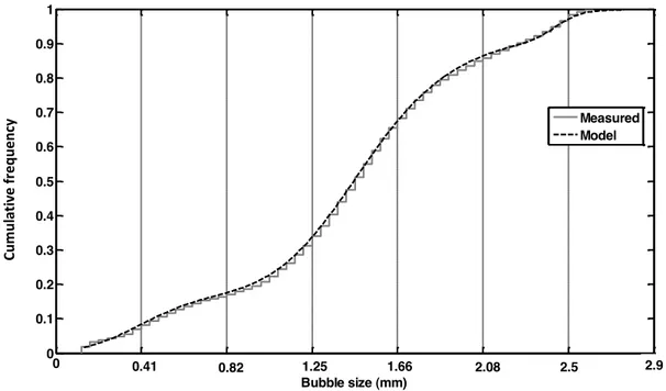
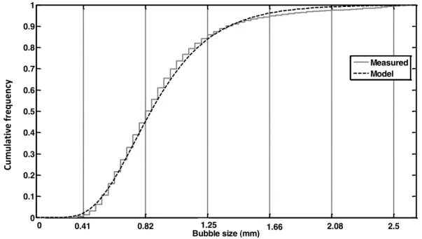
Table 4.1 Experimental conditions for three types of BSD ... 88
Table A.1 Measured RTDs of the tests ... 140
Table B.1 Effect of temperature and duration of test on bubble size distribution ... 142
Table B.2 Values of hydrodynamic variables generated by manipulating Jg and Jsw ... 143
Table C.1 XRF results of quartz (%) ... 147
Table C.2 Mineralogy analysis results ... 148
Table C.3 XRF results for quartz particles (%) ... 149
Table F.1 Experimental results ... 160
Table F.2 Gorain's results ... 161
Table F.3 Massinaei et al. data base ... 162
Table F.4 Kracht et al. data base ... 163
xiii
List of Figures
Figure1.1 Distribution of radial components of the particles and liquid velocity on the
bubble surface ... 7
Figure 1.2 Mechanical cell schematic (Fuerstenau et al., 2007) ... 11
Figure 1.3 Flotation column schematic ... 12
Figure 1.4 Three layers of the froth zone ... 14
Figure 1.5 Typical grade–recovery curves for froth flotation ... 17
Figure 1.6 Different bubble size distributions all having the same d32 ... 26
Figure 1.7 Different pairs of bubble size and gas velocity leading to a unique BSAF ... 31
Figure 1.8 Two BSDs having same d32 originate different kinetic constant ... 32
Figure 1.9 Light beam passing through loaded bubble ... 35
erugiF 2.1 Schematic of the experimental set-up ... 44
Figure 2.2 Schematic of the εg sensor (Gomez et al., 2003) ... 45
Figure 2.3 Schematic of a frit-sleeve sparger (Kracht et al., 2008) ... 46
Figure 2.4 Example of an original captured image and detected bubbles ... 47
Figure 2.5 Effect of the solid percent on the bubble size distribution ... 49
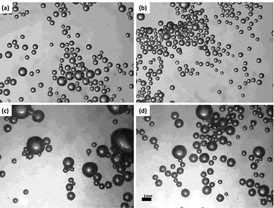
Figure 2.6 Example of bubble images using 25 ppm F150, and for Jg = 1 cm/s ... 50
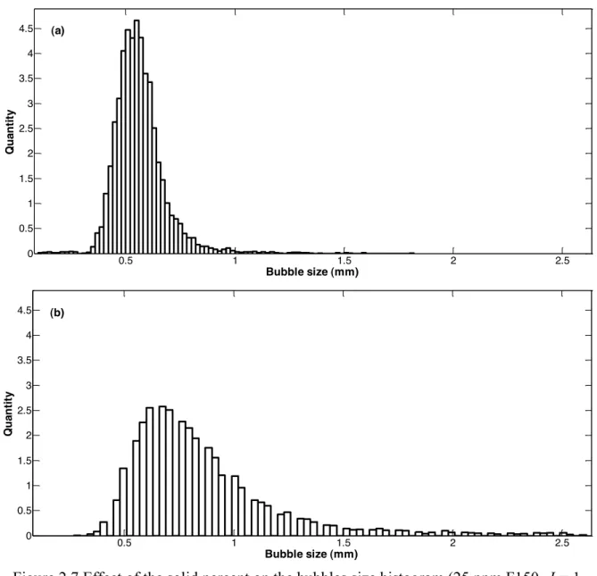
Figure 2.7 Effect of the solid percent on the bubbles size histogram ... 52
Figure 2.8 Bi-modal distribution due to coalescence ... 53
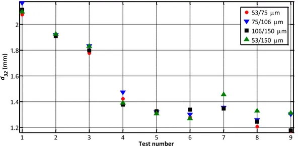
Figure 2.9 The effect of the particle size on the bubble d32 at constant gas rate (1 cm/s) .... 54
Figure 2.10 The effect of solids on the parameters of the bubble size distribution ... 57
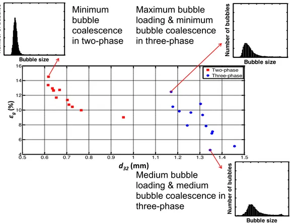
Figure 2.11 Bubble size and gas hold-up correlation in two and three-phase system ... 60
xiv
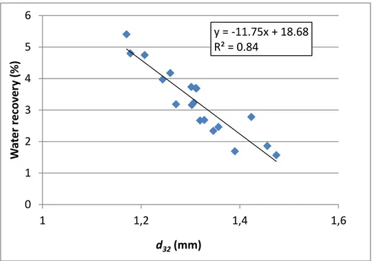
Figure 3.1 Effect of the mean bubble size (d32) on water recovery for constant as rate ... 68
Figure 3.2 Effect of the gas hold-up on the water recovery for constant as rate ... 68
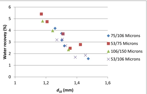
Figure 3.3 Effect of the mean talc particle size on the water recovery ... 69
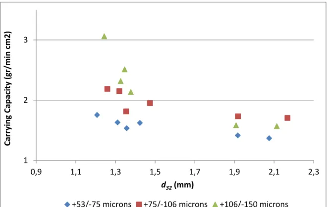
Figure 3.4 Effect of (a) the bubble size, (b) gas holdup, and (c) bubble surface area flux on the carrying capacity ... 71
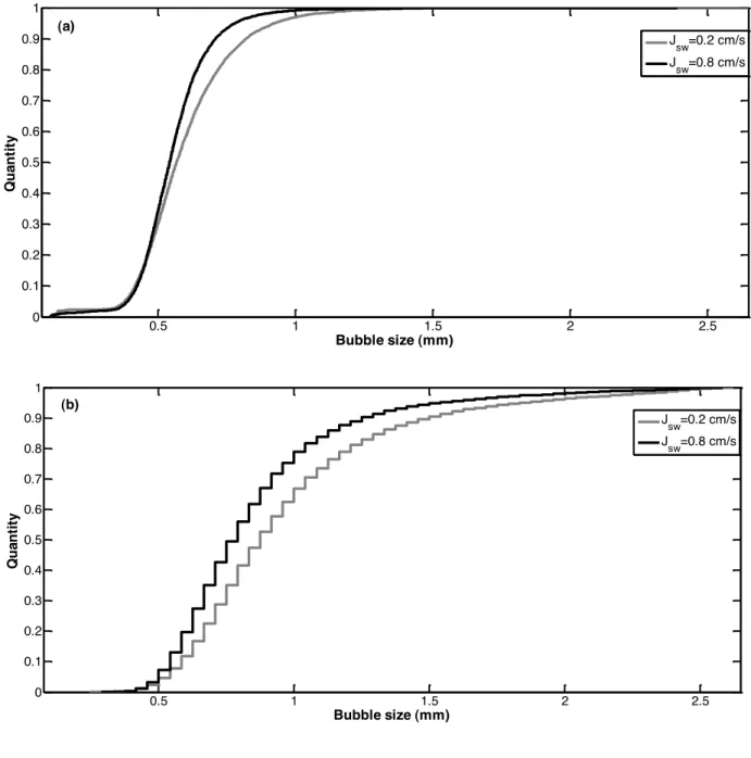
Figure 4.1 Bubble size distribution histogram ... 85
Figure 4.2 Example of a bubble size histogram for T1 distribution ... 86
Figure 4.3 Example of a cumulative bubble size T2 distribution fitted with multi-shape density function ... 87
Figure 4.4. Example of a cumulative bubble size T3 distribution fitted with a lognormal density function ... 88
Figure 4.5 Shows the correlation between Ibc and Ibm (a) for T2 distribution (b) for T3 distribution ... 89
Figure 4.6 Correlation between : (a) Ibc and Sb for T2 distributions, (b) Ibc and Sb for T3 distributions, (c) Ibm and Sb for T2 distributions, (d) Ibm and Sb for T3 distributions ... 90
Figure 4.7 Correlation between: (a) Ibc and εg for T2 distributions, (b) Ibc and εg for T3 distributions, (c) Ibm and εg for T2 distributions (d) Ibm and εg for T3 distributions ... 91
Figure 5.1. Relative importance of particle size (P.S.), εg, Sb and Ib ... 101
Figure 5.2. Importance of variables in VIP projection for three sizes of particles ... 104
Figure 5.3 PLS regression for hydrodynamic variables ... 105
Figure 5.4. PLS regression for hydrodynamic variables ... 106
Figure 5.5 PLS regression for hydrodynamic variables ... 107
Figure 5.6 PLS regression for hydrodynamic variables ... 107
Figure 5.7 PLS regression for hydrodynamic variables using mixed-size class particles . 108 Figure 5.8 PLS regression for hydrodynamic variables ... 109
xv
Figure 6.1 Talc collection rate constant as a function of the bubble size ... 114
Figure 6.2 Talc collection rate constant as a function of Sb for two particle size-classes .. 114
Figure 6.3 Kinetic constant as a function of d32 for the collection zone and the overall process ... 115
Figure 6.4 Nonlinear regression for d32 and kinetic constant, Predicted and actual values 117 Figure 6.5 Nonlinear regression for Sb and kinetic constant, Predicted and actual values . 118 Figure 6.6 Flotation rate constant as a function of εg for large particle size-class ... 119
Figure 6.7 Predicted and actual kinetic constants for the 106/150 µm particle size-class . 120 Figure 6.8 Flotation rate constant as a function of Ib for large particle size-class ... 120
Figure 6.9 Linear regression for Ib and k for large range particle size-class ... 121
Figure A. 1 shows the sampling points from flotation column .... ...137
Figure A. 2 schematic of sampler and its position in the column ... 138
Figure A. 3 Example of measured RTD by conductivity cells; Left) tracer impulse in the feeding point, Right) the detected response of tracer in the tailing point ... 139
Figure B. 1 Bubble size variation by shear water to a frit and sleeve sparger ... ...141
Figure B. 2 d32 variations over time ... 142
Figure B. 3 a) Variations of d32 with the gas and shearwater rates, b) variations of εg with the gas and shearwater rates and c) variations of Sb with the gas and shearwater rates .... 145
xvii
Nomenclature
BSD bubble size distribution f(db) size distribution function
c concentrate assay Ib interfacial area of bubbles
C total concentrate weight Ibc calculated Ib
db bubble size Ibm predicted Ib from d32 and εg
db max maximum bubble size Jg superficial gas rate
db min minimum bubble size k flotation rate constant
d0 bubble size at Jg = 0 µ mean of the BSD
d10 mean diameter of the BSD PC collision probability
d32 Sauter mean diameter of the BSD PD detachment probability
EA attachment efficiency R recovery
Ec collision efficiency Re Reynolds number
Ek collection efficiency Rp particle radius
erf (x) error function Sb bubble surface area flux
εg gas hold-up t assays of the tailing
f assays of the feed tind induction time
F total feed weight tslide sliding time
xix “Whatever you look for-will become your core” 1
To my immortal beloved ones: my parents
xxi
Acknowledgments
I would like to sincerely thank my supervisor, Professor Rene del Villar, for his guidance, support, and insightful comments throughout the years. Under his tutelage, I have learned to question myself and to think more sophisticatedly in order to perform quality research. As a mentor, his contributions to my professional development are invaluable.
Special thanks are likewise expressed to Professor Jocelyn Bouchard, my Co-supervisor, for providing perspective that contributed significant to this work. I am grateful for his diligent efforts to mentor me in many directions throughout my years as a PhD student. I would like to express my gratitude towards Professor Claude Bazin for their thought-provoking comments.
I would like to extend my gratitude to Jonathan Roy and Alberto Riquelme Diaz for their dedicated cooperation at the beginning of this research. Special thanks to Vicky Dodier for assistance in setting up the apparatus and technical support. I would like to acknowledge Dr. Massoud Ghasemzadeh Barbara and Professor Carl Duchesne for cooperating on the statistical analysis of the data.
I acknowledge the financial support received from NSERC (Natural Sciences and Engineering Research Council of Canada) and Corem, throughout my studies at Laval, Finally, I am forever thankful for the encouragement and support from my family, especially my parents, Dr. Damavandi and Dr. Amir Vasebi without whom this endeavor would not have been possible.
xxiii
Foreword
Chapter 2 is based on the article "Effect of particles on the bubble size distribution and gas hold-up in column flotation" submitted in October 2014 to the International Journal of Mineral Processing authored by Ali Vazirizadeh, Jocelyn Bouchard and Yun Chen. This article presents some explanations for the solid particle effects on bubble size and gas hold-up through the investigation of micro-phenomena. My role in the preparation of this article is that of main writer supervised by the co-authors for corrections.
Chapter 3 uses the material of the article "The effect of gas dispersion properties on water recovery in a laboratory flotation column" accepted and presented by myself at the 2014 IMPC Conference, Santiago, Chile, from 20-24 October 2014. I participated in the writing as the first author, followed by Jocelyn Bouchard and Rene del Villar who contributed to the editing of this document. The main objective is to study the effect of the gas rate, gas hold-up, bubble size and bubble surface area flux on the water recovery to the concentrate. I performed the laboratory testwork and analysis under the supervision of professors. Bouchard and del Villar.
Chapter 4 is based on the article "On the relationship between hydrodynamic characteristics and the kinetics of column flotation. Part I: modeling the gas dispersion". The interfacial bubble area concept is introduced in this article as a new hydrodynamic variable; its correlations with the other hydrodynamic variables are presented. This article was accepted for publication in Minerals Engineering in September (2014). I did all the laboratory, data analysis and mathematical developments. I participated in the writing as the first author. My co-authors, Professors Jocelyn Bouchard and del Villar corrected and edited the manuscript.
Chapter 5 uses the material presented in the article "On the relationship between hydrodynamic characteristics and the kinetics of flotation. Part II: model validation". The correlation between the flotation rate constant and particle size as well as some hydrodynamic variables is investigated in this article. This article was accepted for publication in Minerals Engineering in November (2014). My contribution as the first
author was performing the testwork, analyzing the data and writing the manuscript. Mr. Ghasemzadeh Barbara and Prof. Duchesne of Chem. Eng. Dept. contributed to the statistical analysis using PLS. Professors Bouchard and del Villar supervised the data analysis, as well as the preparation and edition of the article.
1
Chapter 1 Introduction
1.1 Principles of flotation
Froth flotation is a mineral separation method based on differences in water-repellency characteristics of the various mineral species contained in aqueous slurry. The hydrophobic particles attach to gas (generally air) bubbles injected at the bottom of the separation vessel. As a result of their lower specific gravity, the bubble-particle aggregates ascend to the vessel slurry surface, whereas the hydrophilic particles, that remain completely wetted, stay in the liquid phase and therefore are removed from the bottom of the device. Froth flotation can be practiced for a broad range of mineral separations, as it is possible to use chemical treatments to selectively modify mineral surface characteristics so that they have the required hydrophobicity for the separation to occur. Some examples are separation of sulfide minerals from siliceous gangue, separation of coal from ash-forming minerals and removing silicates from iron ores. Flotation is also used in chemical engineering fields such as processing recycled printed papers, where ink (carbon) is separated from paper-pulp; it is also used in the oil production from tar sands, where oil (carbon derived) is removed from sand (siliceous gangue). Flotation is particularly useful for processing fine-grained ores that are not amenable to other physical separation methods such as gravity- or magnetic-based methods.
1.2 Hydrophobic and hydrophilic particles
In terms of their behaviour in an aerated liquid (water), particles can be classified in two groups: those that are readily wettable (hydrophilic) and those that are water-repellent (hydrophobic). If a mixture of hydrophobic and hydrophilic particles is suspended in water contained in a device where air bubbles are injected, the hydrophobic particles will tend to attach to the bubbles and float with them to the top of the device (called a flotation cell) where they accumulate as a persistent froth, heavily loaded with the hydrophobic mineral, wherefrom it can be removed as a product, usually a valuable mineral concentrate. Since hydrophilic particles do not attach to the air bubbles, they will remain in the suspension, flowing down to the bottom exit of the cell, as a refuse (tail).
2
1.3 Use of reagents in flotation practice
With very few exceptions, minerals are rarely suitable for froth flotation, because they are naturally hydrophilic. Among the exceptions (natural hydrophobic minerals), it can be mentioned coal and carbon derivatives (like oil, diamonds, graphite), native sulphur, molybdenite and talc (used in this thesis as the hydrophobic component). Chemical reagents are thus required to render hydrophobic the target (valuable) hydrophilic mineral and also to preserve suitable froth characteristics.
1.3.1 Collectors
Collectors control the selective attachment of particles onto the bubble surface. They form a monolayer on the particle surface, which essentially leads to generate a thin film of nonpolar hydrophobic hydrocarbons, rendering the mineral surface hydrophobic. Selection of the correct collector is important for an effective separation by flotation. Collectors are generally classified depending on their ionic charge. They can be anionic, cationic, or non-ionic. The anionic and cationic collectors contain a polar part, which selectively attaches to the mineral surfaces and a non-polar part (organic), which projects out into the solution, making hydrophobic the particle surface. Non-ionic collectors are hydrophobic products (hydrocarbon oils, grease), which adhere to the surface forming a physical coat repelling water. Collectors can either chemically cover the mineral surface (react with) or they can be bonded on the surface by physical forces.
In the chemical coverage case, ions or molecules from the solution undergo a chemical reaction with the surface, becoming strongly bonded. This process drastically changes the nature of the surface. These kinds of collectors are highly selective, as the chemical bonds are specific to particular atoms. Among them Xanthates are the most commonly used collectors for sulfide mineral flotation.
In the case of physical coverage, ions or molecules from solution are reversibly linked with the surface, the attachment is due to electrostatic attraction or Van der Waals bonding. These collectors can be desorbed from the surface if some conditions change, such as variations in pH or in the solution composition. The collectors, bonded through physical coverage, are much less selective than the collectors chemically attached, as they might
3 adsorb on any surface that has the correct electrical charge or degree of natural hydrophobicity. The collector available for the flotation of oxide minerals (oxyhydryl collectors) are one of those. Typical examples are the fatty acid salts, e.g. sodium oleate, the sodium salt of oleic acid.
1.3.2 Modifiers
Modifiers are chemical reagents changing the form the collector attaches to the mineral surface. They are categorized in: (a) activators, which increase the adsorption of collector onto a given mineral, (b) depressants, that prevent collector from adsorbing onto a mineral and (c) pH-regulators.
The latter are probably the simplest type of modifiers, since the surface chemistry of most minerals is determined by the pH. For example, minerals in general exhibit a negative charge under alkaline conditions and a positive surface charge under acidic conditions. Since each mineral change from negative charge to positive charge at some particular pH, it is possible to control the degree of attraction of collectors to their surfaces simply by pH adjustments. Acids are used generally to adjust pH in the low range, while alkalis such as lime (CaO or Ca(OH)2) are used to rise pH. Pyrite can be separated from chalcopyrite by
regulating the suspension pH to an appropriate value.
The possibility of collector attachment increases by means of activators, i.e. activators facilitate the task of a collector. A classical example of an activator is the use of copper sulfate as an activator for sphalerite (ZnS) flotation with xanthate collectors. The copper ions replace the zinc ions on the surface and the xanthate gets fixed more effectively to the newly formed ”copper” surface, rendering the Cu-coated ZnS particle hydrophobic.
Depressants act by preventing collectors from attaching onto particular mineral surfaces, thus they show the opposite effect of activators. For example, cyanide ions act as particularly useful depressant for pyrite (FeS2) during sulfide minerals flotation.
1.3.3 Frothers
Frothers are compounds that help changing the size and stabilizing the generated bubbles, so that they remain well dispersed in the slurry and form a stable froth layer, which can be
4
removed before bubble bursting. Many types of organic compounds serve this objective. However, some of them have also collecting properties (e.g. amines, carboxylic acids, etc.). In such cases, their dosage control might become cumbersome (same reagent having two different actions). This is why the most commonly used frothers are alcohols, which do not have collecting properties. The most commonly frother used in plant practice are the methyl isobutyl carbinol (MIBC) and water-soluble polymers, such as polypropylene glycols and polyglycols (F150). The polypropylene glycol frothers in particular are very versatile and they can be manipulated to a wide range of froth properties. Some other frothers available are natural product such as cresols and pine oils; however most of them are considered obsolete, because of their cost, and are not as widely used as the synthetic ones.
1.4 Bubble-particle collection
The basic flotation separation mechanism is hydrophobicity, which is the ability of a given particle to get attached to an air bubble after a collision. However, such separation mechanism is not perfect, as some undesired particles (low-grade non-liberated) might attach to the bubbles or are entrained in the bubble wake entering into the froth zone. Inversely, some hydrophobic particles might detach from the air bubbles during the transport of the bubble-particle aggregates to the froth zone or due to bubble coalescence in it, thus returning back to the pulp phase; also some hydrophobic particles do not attach to the bubbles because of their size (too small or too large) and the number of available bubbles (amount of bubble surface).
In a flotation device, a mineral particle is collected by an air bubble through one of two main mechanisms: 1) particle-bubble attachment due to the particle surface hydrophobicity, or 2) entrainment into the wake of the bubble and the boundary layer which does not relate to the particle hydrophobicity.
The particle collection by attachment occurs due to bubble-particle collision followed by adhesion of the hydrophobic particle on the surface of air bubble. The efficiencies of both steps determine the final collection efficiency by attachment. However, there is another micro process to be considered, called detachment. The detachment usually occurs when
5 the particle-bubble is disrupted by flow turbulence or bubble coalescence. Consequently, the collection efficiency, Ek, is given by:
Ek = Ec EA (1- PD) (1-1)
where Ec is the collision efficiency, EA is the attachment efficiency, and PD is the
detachment probability.
1.4.1 Bubble-Particle Collision
The collision efficiency is the fraction of all hydrophobic particles swept out by the projected area of bubbles that collide with the bubbles.
Yoon (1993) explained that the collision efficiency is strongly affected by both the particle size and bubble size as well as by the system turbulence. He introduced a model between collision efficiency and bubble size and particle size under different hydrodynamic conditions:
( / )n
c p b
P A d d (1-2)
where dp is the particle size diameter, db is the bubble mean size diameter, A and n are
model parameters depending on the flow conditions. Table 1.1 indicates the value of those parameters for each flow condition, depending on the bubble Reynolds number (Re). He quantified how increasing the bubble size decreases the probability of collision regardless of the flow conditions.
6
Table 1.1 Yoon’s model parameters for different flow conditions
Flow condition A n Stokes 2/3 2 Intermediate 3 4 0.72 2 15 Re 2 Intermediate 3 1 (3 /16) 0.56 2 1 0.249 Re Re 2 Potential 3 1
Based on experimental observation, Finch and Dobby (1990) indicated that when particle size increases, collision efficiency also increases, but attachment efficiency decreases. This is in accordance with Yoon's model (Eq. 1-2) and common knowledge. Dai et al. (2000) came to the same conclusion as Finch and Dobby (1990), based on reviewing the previous collision models.
Independently of the size of the particle being floated, large bubbles exhibit lower collection efficiencies than fine bubbles. However, using very fine bubbles does not improve the process selectivity because the possibility of particle-bubble collision for fine and coarse particles are relatively similar (Dobby and Finch, 1987).
Weber and Paddock (1983) studied the particle-bubble collision based on the equation of motion of spherical particle relative to a spherical bubble rising in an infinite pool of liquid. According to their study, the collision efficiency is affected by two main steps: first, by intercepting collisions, occurring for neutrally buoyant particles exactly following the fluid streams, and second, by gravitational collisions which would occur for particles with assumed zero dimension and finite settling velocity. The efficiency of both steps increase by increasing the particle size and decreasing the bubble size.
7 The collection efficiency improves as a result of increasing the collision independently of the attachment efficiency. Therefore, regarding Weber and Paddock's conclusion, the collection efficiency would increase by generating finer bubbles.
1.4.2 Particle attachment
A key concept in the estimation of particle–bubble attachment probability is the induction time, tind, first introduced by Sven-Nilsson (1934). Basically, the induction time is defined
as the sliding time of a particle on the bubble surface required for thinning and draining the liquid film interposed between the particle and the bubble, until its rupture and actual contact between particle and air bubble. In the flotation process, the induction time can be interpreted as a threshold sliding duration (Nguyen and Schulze, 2003). When a particle meets a bubble, it will first deviate from its initial trajectory, due to fluid forces, and then it will slide on the bubble surface for a short period of time called tslide. If tslide equals or
exceeds tind, then attachment is expected to occur. The tslide depends on the distribution of
bubble-particle collision angles, the maximum bubble-particle contact angle and the particle sliding velocity (Finch and Dobby, 1990). The particle collision angle is determined from the angle made by the fluid streamlines and the bubble in the vicinity of the bubble surface (Figure 1.1).
The maximum contact angle corresponds to the angle where the radial component of particle settling velocity (directed toward the bubble surface) is equal to the radial component of the liquid velocity (oriented away from the bubble surface).
Figure1.1 Distribution of radial components of the particles and liquid velocity on the bubble surface
θ θ
max
Radial component of particle settling velocity
8
Moreover, Yoon (1993) stated that surface chemistry and system hydrodynamic conditions have an enormous effect on the induction time, which is mainly determined by the particle hydrophobicity. According to Yoon, For example, for two same-size mineral particles, the strongly hydrophobic could have an induction time of around 15 ms, whereas the second one, weakly hydrophobic, would require 40 ms for induction.
The reduction of particle size, for a given bubble size, may have an effect on flotation selectivity. Longer sliding times give more chances to any particle to attach to bubbles, irrespective of their degree of hydrophobicity. In other words, less hydrophobic particles (containing some gangue at the surface) can have similar chances to attach to the bubble as highly hydrophobic (richer) particles. Consequently, both sorts of small particles may attach to the bubble and selectivity is then reduced.
On the other hand, selectivity increases if bubble size diminishes since the sliding time may be too short compared to the induction time (Weber and Paddock, 1983).
While the collision process is more determined by physical parameters, adhesion is the result of both physical and chemical factors. Since both the bubble size and particle size affect collision and adhesion, the effect of these two variables is more pronounced on collection efficiency.
1.4.3 Particle detachment
A particle will be detached from an air bubble if the detachment force exceeds the attachment force. The maximum attachment force of a single particle can be calculated from:
cos
a p
F =π σ R 1- θ (1-3)
where Fa is the attachment force, Rp is the particle radius, σ the liquid surface tension and θ
the three-phase contact angle (Nutt, 1960).
The detachment force is the sum of gravitational forces, shear forces and external vibratory forces, the latter depending on the particle mass, the vibration amplitude and frequency (Cheng and Holtham, 1995). The particle size and flow turbulence in flotation – the latter mostly determined by the flotation device – affect on each individual detachment force.
9 However, in general, the probability of detachment is less important in a flotation column than in a mechanical cell, because the flow turbulence in the flotation column is much lower than in a mechanical cells (Finch and Dobby, 1990). In addition, the probability of detachment of fine particles (less than 100 μm) is mostly negligible.
1.4.4 Particle entrainment
According to Cilek (2009), the entrainment mechanism not only refers to the recovery of hydrophilic particles but also to hydrophobic particles recovered without being attached to air bubbles. The particle entrainment is directly related to the fraction of water reporting to the concentrate, called ‘water entrainment’. There is agreement in that the wake of the bubble swarm is responsible for the water entrainment to the froth. The volume of the bubble wake is a function of the bubble size and its rising velocity, as well as the liquid viscosity, therefore the water entrainment should be determined by such variables.
The role of frother type and concentration (as the manipulated variable in flotation) on water entrainment can be illustrated through its effect on the bubble size and velocity
(Ekmekçi et al., 2003). Since frother modifies the bubble size and its velocity, it indirectly determines the bubble wake and consequently the volume of water reporting to the concentrate.
In addition, it appears that gas dispersion properties in general (such as the bubble size, gas hold-up, etc.) play a major role, similar to the frother effect, on the particle entrainment through their effect on bubble wake (Nelson and Lelinski, 2000; Phan et al., 2003; Rodrigues et al., 2001; Yoon, 2000).
Yianatos et al. (2009) observed a selective entrainment of fine particles (less than 45 μm) in a large industrial cell as. On the other hand, the recovery of coarse particles (larger than 150 μm) by entrainment is considered negligible, less than 0.1% (Yianatos et al., 2009; Zheng et al., 2006). Experimental evidence also confirms that if the liberation size is smaller, grinding product (cyclone overflow) must be finer which might imply a greater content of fine gangue particles, easier to be entrained than coarser ones (Guler and Akdemir, 2012).
10
Regarding to the micro-processes presented in this section (1.4), it seems that the bubble size and particle size, as well as the flow conditions in the flotation device, play the most important role on particle recovery when particles have the same hydrophobicity.
1.5 Flotation devices
The flotation process is accomplished in a device having two main roles: keeping the pulp in suspension and providing air bubbles. The device should also provide a mean to evacuate the two products: concentrate (loaded froth) and tails (depleted mineral pulp). There are two main flotation devices well accepted in the industrial practice, flotation columns (and other similar devices) and mechanical cells. The latter are usually connected in banks having enough cells to assure the required particle residence time for adequate recovery. Subsequently, various banks, each having its particular targets of concentrate grade and recovery, are interconnected to form a flotation circuit, capable of attaining the desired overall metallurgy (product).
1.5.1 Mechanical cells
A mechanical flotation cell is basically a cylindrical or rectangular vessel or tank fitted with an impeller. The impeller function is to mix thoroughly the slurry to keep particles in suspension, and also to disperse the injected air into fine bubbles, providing conditions promoting bubble-particle collisions. It is worth mentioning that mechanical cells operate either on self aspiration mechanism (no air feed rate control) or controlled compressed air. Formed bubble-particle aggregates rise up through the cell by buoyancy and are removed from it into an inclined drainage box called "concentrate launder". Water sprays will help breaking the aggregates to make possible the pumping of the concentrate downstream. Particles that do not attach to the bubbles are discharged out from the bottom of the cell.
A mechanical cell requires the generation of three distinct hydrodynamic regions for effective flotation. The region close to the impeller encompasses the turbulent zone needed for solids suspension, dispersion of gas into bubbles, and bubble-particle interaction. Above the turbulent zone lies a quiescent zone where the bubble-particle aggregates moves up in a relatively less turbulent area. This zone also helps in sinking the amount of gangue minerals that may have been entrained mechanically. The third region above the quiescent zone is
11 the froth zone serving as an additional cleaning step as a result of bubble coalescence and other phenomena (Fuerstenau et al., 2007). Figure 1.2 shows a typical schematic of mechanical cell.
Figure 1.2 Mechanical cell schematic (Fuerstenau et al., 2007)
1.5.2 Flotation columns
A flotation column is typically a tall vertical cylinder or rectangular with no mobile parts (agitator), fed with a mineral pulp (top third of column), air bubbles is injected (always generated by controlled compressed air) at its very bottom. These bubbles rise-up in counter-current with the descending flow of pulp, so that the contained hydrophobic particles are able to attach to the air bubbles. The so-formed bubble-particle aggregates are carried upwards by a buoyancy effect. The zone where this process takes place is called the collection zone, corresponding to 75% to 90% of the total column height. The hydrophilic particles and some non-collected hydrophobic particles move downwards throughout the collection zone, being finally discharged through the tailing outlet at the bottom of the column. The ascending bubble-particle aggregates accumulate in the upper part of the
12
column before overflowing into a launder as a concentrate. This zone, which stands from the pulp-froth interface up to the top of the column, is called the froth zone or cleaning. Its thickness generally varies between 10% and 25% of total column height (Zheng, 2001 ), although in specific applications it can be as shallow as 40 cm. Figure 1.3 shows a schematic of a flotation column unit.
Figure 1.3 Flotation column schematic
1.5.2.1 Bubble generating systems
The bubble size is essentially determined by the type of frother and the mechanism used for bubble generation. It can be modified through the frother concentration, and gas feed rate to the device. The bubble generation system is another feature which distinguishes flotation columns from mechanical cells. In the case of flotation columns the most commonly used for bubble generation method is through internal spargers near to the bottom of the device. There are two categories of internal spargers: porous spargers and single or multinozzle spargers (Finch and Dobby, 1990). Whereas the former are used at laboratory scale, the second method is the most common at industrial scale. A variant has been introduced in the
Feed Conc Tail Water Air Wash Water
13 so-called reactor-separator columns, in that gas and slurry are brought into intense contact in an external section (called reactor), with a very short residence time. Then the aeratered pulp passes to a quiescent zone (separator) where bubble aggregates separate from settling gangue particles, each stream exiting the separator at a different outlet. The amount of slurry introduced to the sparger is usually a small fraction of tails flow rate (around 10%) (Massinaei et al., 2009).
In the mechanical cells,air enters to the device through a concentric pipe surrounding the impeller shaft. The rotating impeller tips create a high-shear zone where air is broken up into a dispersion of bubbles, when passing through a static set of bars around the impeller. The bubbles are deviated outwards from the impeller tips and dispersed throughout the solid-liquid mixture (slurry) into the next zone (quiescent) of the cell (Fuerstenau et al., 2007).
1.5.2.2 Froth zone, wash water and bias rate
Another feature distinguishing the flotation column from the mechanical cell is the addition of wash water above or slightly inside the froth zone. A fraction of this flow of fresh water travelling down the froth zone, would wash-out the hydrophilic particles entrained into the froth zone, thus avoiding their recovery to the concentrate. The remainder of the water injected helps the concentrate overflowing into its launder. To assess the wash water cleaning performance, the bias rate concept – i.e. the fraction of the wash water flow rate going downwards through the pulp-froth interface – was introduced by Finch and Dobby (1990).
14
Figure 1.4 Three layers of the froth zone
The froth zone normally consists of three regions: an expanded bubble bed (next to the interface), a packed bubble bed above the previous one and a conventional draining froth at the top (Figure 1.4). As for practical considerations (plugging of water nozzles) wash water is sometimes sprayed above the froth and therefore the conventional draining froth does not establish properly (Finch and Dobby, 1990).
Bubbles pass through the collection zone and enter the expanded bubble bed after colliding with the first layer of bubbles, which defines a very distinct interface. These incoming bubbles have a relatively homogeneous and small size and remain spherical all the way up. Bubbles colliding with the interface, generate shock pressure waves promoting collisions up through the expanded bubble bed. This phenomenon seems to be the main cause of bubble coalescence, promoting film thinning and finally its rupture.
The packed bubble bed region expands to the wash water inlet level. The fractional liquid content is lower than in the expanded bubble region and bubbles keep a relatively spherical shape, but the range moves towards larger bubbles. Bubbles rise upward with close to plug-flow conditions, thus promoting a good distribution of the wash water.
Expanded bubble bed Packed bubble bed Conventional draining froth
15 Above the wash water inlet level lays the conventional draining froth, therefore the net flow of water is ascending here is negative. The main aim of this region is to convert froth vertical motion into horizontal motion to collect the froth.
1.6 Flotation modeling
1.6.1 Performance justification
There is no universal way for expressing the effectiveness of a separation, but several useful indices exist for evaluating the quality of the flotation process.The following are the most commonly used.
Ratio of concentration: defined as the weight of feed divided by the weight of concentrate, that is:
ratio of concentration = F/C (1-4)
where F is the total feed weight and C is the total concentrate weight .
The drawback of this performance index is the need of weight values. Although from laboratory experiments these data can be obtained, in the industrial practice it is unlikely that the ore is weighed, only assays are available. However, is possible to express the ratio of concentration in terms of ore assays. From the definition of the ratio of concentration (F/C) and using the following mass balance equations, it can be calculated:
F= C+T (1-5)
Ff=Cc +Tt (1-6)
where f, c, and t are assays of the feed, concentrate, and tailings, respectively. Rearranging Eq. (1-5) and Eq. (1-6) gives:
c t F C f t (1-7)Percent recovery: The percent recovery is the percent of mineral in the original feed that is recovered in the concentrate. By means of weights and assays it can be calculated by:
16 100 C c R F f (1-8)
or by replacing weights by assays (from material balances):
100 c f t R f c t (1-9)where R is the percent recovery.
Enrichment ratio: The enrichment ratio is directlycalculatedfrom the assays as c / f. Mass pull: The mass pull is the inverse of the ratio of concentration, thus:
f t C F c t (1-10) Grade-recovery curvesAlthough the above mentioned indices are useful for comparing flotation performance for different conditions, a “grade–recovery curve”, constructed from concentrate grade and recovery values at different operating conditions, is a more useful tool for inferring the optimal operating conditions. This is a graph of the recovery of the valuable mineral against the concentrate grade for given operating conditions, and it is particularly practical for comparing separations where both the grade and the recovery are varying. A set of grade– recovery curves is shown in Figure 1.5.
17 Figure 1.5 Typical grade–recovery curves for froth flotation
Controlling of grade and recovery in flotation processes has received significant attention from researchers in the past years. Since more than hundred variables affect the flotation process (Arbiter, 1962), knowing which variables have more influence, can help controlling flotation performance variables, i.e. the grade and recovery. On the other hand, finding the relationship between manipulated variables and controlled variables is imperative to find out set-points leading to improved metallurgy. Therefore, some models for recovery parameters have been proposed. The form of such models and their definition are presented in the next section.
Another important parameter often used for cell/column design is the so-called carrying capacity. The carrying capacity of the cell is calculated based on the recovered mass of particles, both hydrophobic and hydrophilic, per unit cell surface per unit of time. This
Improving
Performance
Pure
Mineral
Assay (%)
Feed
100
0
Rec
ov
ery (
%
)
18
variable is directly related to the bubble surface available for collection, and therefore to the bubble size. 2 1 ( ) min dC kg Carrying Capacity dt A m (1-11)
where A is the cross-section area of the flotation cell and t is the time unit and C is total recovered mass.
1.6.2 Kinetic constant modeling
To model the flotation process, two main approaches are possible: the empirical modeling and the phenomenological modeling.
In empirical models, input and output variables are related through suitable mathematical equations. Statistical methods are used to define dependent and independent variables and to estimate the curve fitting parameters. Obtained parameters do not necessarily have any physical meaning and they are valid just for the limited conditions in which the model was calibrated.
Phenomenological modeling provides an explanation for causes and effects, which are related to physical and chemical conditions of the process. Phenomenological models are divided in three main categories: kinetic, probabilistic and population balance models. Probabilistic models are based on some sub-processes such as collision, adhesion and detachment and can be used as a bridge between micro- and macro-models. Kinetic models use the chemical reactor analogy and consider flotation as a reaction between bubbles and particles (Polat and Chander, 2000). A good understanding about mixing conditions in the flotation process is also required to obtain a reliable kinetic model. For instance, mixing conditions in a laboratory column (5 cm diameter) are close to plug flow pattern, whereas in industrial columns they are something between plug flow and perfect mixing patterns (Finch and Dobby, 1990).
There is an expression relating the collection efficiency to the flotation rate constant. For the situation of gas bubbles rising through a column of water containing hydrophobic particles at a concentration cp and having collection efficiency Ek, and given a cubic volume
19 of water with side dimension L, the particle collection process is represented by the rate of particle removal from the slurry by air bubbles. In other words, it can be calculated from the rate of particle removed per bubble times the number of bubbles.
At a gas rate Qg and a slip velocity Usg (the velocity of gas relative to slurry), this
expression is equivalent to:
2 3 3 4 6 p b g sg p k sg b dc d Q L L U c E dt d U (1-12)After cancelling out some terms: 1.5 p g k p b dc J E c dt d (1-13) where 2g g Q J L .
Eq. (1-13) is equivalent to the expression of first-order rate process where the first order rate constant kc is given by:
1.5 g k c b J E k d (1-14)
It is very well accepted that the flotation process follows a first order kinetics with respect to the concentration of the floatable particles c as indicated in equation (1-15).
dc
k c
dt (1-15)
By integration and introduction of the recovery definition, it is possible to obtain the following expressions, respectively for plug flow conditions (Eq.1-16) and perfect mixing conditions (Eq.1-17):
(1
)
kcR
e
(1-16) 1 c c k R k
(1-17)20
where τ is the particle mean residence time. Equation (1-16) for plug flow and Equation (1-17) for perfect mixture indicate that increasing the flotation kinetic constant leads to an increase in the recovery.
In the case of plug flow conditions (or a batch flotation processes), equation (1-16) is always valid since the kinetic constant is invariant. However in actual flotation conditions, particle size and bubble size are present as a population distribution, which leads to consider a kinetic constant distribution for proper flotation modeling. It is also possible that the industrial flotation device exhibits a mixing behaviour which is neither plug flow, nor perfect mixing, in which case the residence time distribution, obtained through tracer tests, must be used.
In this regard, Polat and Chander (2000) applied a generalized form of equation (1-16) shown in 0 0 (1 kt) ( ) ( ) R e F k E t dk dt R
(1-18)where R is the mineral recovery at time t and R∞ represents the ultimate recovery at infinite
time, E(t) is residence time distribution and F(k) is the kinetic-constant distribution function for a continues process. This formulation is more appropriate since both the kinetic constant distribution and the residence time distribution are being considered.
It is worth mentioning that the presented recovery models are for the collection zone only; the froth zone recovery has not been considered so far. In fact, as a result of various events taking place in the froth zone (e.g. bubble coalescence) some hydrophobic particle may detach from the bubbles and return to the pulp zone, making the overall recovery lower than that of the collection zone, calculated with the previous equations. To eliminate the froth zone effect on the overall flotation recovery, a very shallow froth height (less than 15 cm) has to be used in the experimental determination of the kinetic constant, so that the overall flotation recovery can be assumed to be equal to that of the collection zone. Since the evaluation of k always implies a series of restrictions or inaccuracies, such as the model will require to be compared to a reference value that is inaccurate. Based on, given all these
21 inaccuracies, a different approach would be worth to be explored. This will be tackled later on in this thesis.
1.6.3 Residence time measurement in a flotation column
One of the most used methods for determining the residence time distribution (RTD) in liquid or pulp systems, is the injection of a know amount of tracer (liquid or solid) at the column feed port and to track its concentration with tailing flow as function of time. Mean residence time can be calculated based on the time variation of tracer concentration through: exp ( ) ( )
i i i erimental i i t C t dt t C C C t dt
(1-19)where τexperimental is the mean residence time (min), C(t) is the tracer concentration at time t.
The expected mean residence time is simply obtained from:
exp eff ected V Q
(1-20)where Veff (m3) is effective cell volume (collection zone without gas) and Q (m3/h) is feed
flow rate.
Various sorts of tracers have been used for RTD measurement, such as ionic salt tracers (NaCl and KCl) and radioactive tracers (Br-82) for liquid RTD and MnO2 as a solid particle
tracer. However, liquid tracers are not as accurate as solid tracers for modeling of flotation because the aim is to track particle behavior in flotation conditions through studying the flotation rate. However, ionic salt tracers are simpler to use as their concentration can be detected by conductivity measurements. These tracers are generally used for liquid RTD measurements as a mean to evaluate the mixing conditions in the flotation device. Radioactive tracers provide more accurate results since less amount of tracer is required and the tracer is tracked by a non-invasive sampling system (measuring the radiation in the output flow).
22
The best tracer for measuring the residence time of solid particles are the solid tracers, as long as they have the same physical features (density, size and hydrophobicity) as the target solid particles. There are some reports on the application of solid tracers like MnO2 for
tracking particle behavior and particle RTD in the flotation cells (Finch and Dobby, 1990). Yianatos and Bergh (1992) have systematically used the radioactive tracer technique for coding the different solid particles and measuring the RTD of hydrophilic particles in industrial flotation columns and cells. More recently, Cole et al. (2010) presented a Positron Emission Particle Tracking (PEPT) method which can be applied to particles in froth flotation systems to observe the behavior of individual hydrophilic particles in a mixed particle–liquid–gas system.
1.7 Gas dispersion properties
Gas dispersion properties have proved to be a key feature of the flotation process. Among them, the most relevant are: the gas hold-up, superficial gas velocity, bubble size and bubble surface area flux. This latter has received considerable attention and has been reported to linearly correlate with the flotation rate constant and bubble carrying capacity, both related to flotation performance (Gorain et al., 1998).
1.7.1 Gas hold-up (εg)
The volumetric fraction of gas in a given volume of the device is called the gas hold-up. For a given column section, it can be estimated through the following equation:
g
Volume of bubbles Volume of aerated pulp
(1-21)
where volume could refer to the total volume of a given zone, in which case we are talking of an overall gas hold-up) or part of it thus a local gas hold-up. The εg value strongly
depends on the prevailing gas rate and bubble size values (Gorain et al., 1998).
1.7.2 Superficial gas velocity (Jg)
The volumetric gas flow rate (cm3/s) divided by the cross-sectional area of the device (cm2)
23 g g Q J A (1-22)
where Qg is the gas volumetric flow rate and A is the cell cross-sectional area. This
definition is quite useful, since is independent of the device size, therefore it is a scalable value. For flotation devices the recommended Jg value should vary from 1-2 cm/s.
1.7.3 Bubble surface area flux (Sb)
Bubble Surface Area Flux (BSAF or Sb) is defined as follows:
surface area of bubbles generated per unit of time cross sectional area of the column
b
S (1-23)
Assuming that bubble sizes can be presented in m different discrete bubble sizes, then Eq. (1-23) can be expressed mathematically as:
1 m i bi i b cell n S S A
(1-24)where Acell is the cell cross sectional area, ni is the number of bubbles of size i generated per
unit of time and Sbi is the surface area of a bubble of size i. Similarly, the volumetric gas
flow rate can be defined as follows:
1 m g i bi i Q nV
(1-25)where Vbi is the volume of an air bubble of size i. Then, Sb can be written as:
1 1 m i bi g i b m cell i bi i n S Q S A nV
(1-26)Assuming that all bubbles are spherical, thenSbi
di2 and 3 6bi i
V d . Since
g g cell
J Q A , Sb can be calculated in terms of the superficial gas velocity Jg and a mean
24 32 6 g b J S d (1-27)
where d32 is the Sauter mean diameter defined as:
3 1 32 2 1 m i i i m i i i n d d n d
(1-28)Another way to calculate d32 from a set of bubble sizes is:
3 1 32 2 1 b b N i i N i i d d d
(1-29)where Nb represents the total number of collected bubbles.
1.7.3.1 Experimental models for Sb
Bubble size measurement in flotation devices is difficult enough to induce researchers to look for simpler alternatives, among which the empirical modeling of Sb has been
considered as the most appropriate approach.
An empirical model was developed by Gorain et al. (1999), using extensive pilot and industrial tests obtained with different cell types and sizes. It allows predicting the Sb in
mechanical flotation cells by
0.44 0.75 0.10 0.42 80
123
( )
b s g sS
N
J
A
P
(1-30)where Ns is the impeller peripheral speed, Jg is the superficial air velocity, As is the impeller
aspect ratio and P80 is feed 80% passing size.
This model was shown to be acceptable for 20-150 µm particles in rougher, scavenger and cleaner mechanical cells, but was not validated for flotation columns (Gorain et al., 1999). Heiskanen (2000) evaluated Gorain’s model and formulated some criticisms. In particular, he mentioned that "the measurement and computation of superficial gas velocity, and partially also the bubble size may be biased in some conditions. This makes the bubble
25 surface area flux behave such that the final outcome is in doubt." Some other criticisms were:
- the model validation did not address the different particle sizes at all;
- the results from Gorain’s evaluation show that increasing bubble size gives a higher flotation rate constant and that poor dispersion gives a good flotation response, both results being in contradiction with earlier finding and industrial experience;
- lastly, he suggested that the bubble surface area flux would need more validation using different ore types and that the linear relationship between flotation rate constant and Sb
also required more research.
Finch et al. (2000) suggested another empirical relationship, this time to predict the Sb from
gas hold-up measurements:
5.5
b g
S
(1-31)This model was tested for mechanical cells and flotation columns, both at laboratory and industrial scale, and it was deemed to be valid for Sb lower than 130 s-1 and εg lower than
25%. The problem of this model is the method used for bubble size estimation (drift flux analysis), which does not have a good accuracy. This Sb prediction model was proposed
based on the fact that gas hold-up measurement is easier than that of the bubble size.
A third expression can be developed using the empirical model proposed by Nesset et al. (2006) for estimating the Sauter mean bubble diameter from superficial gas velocity measurements. They found that the d32 increases when Jg is increased according on:
32 0
n g
d
d
C J
(1-32)where C and n are the model parameters and d0 is determined by extrapolation of the d32
graph for Jg = 0. By replacing the d32 in equation (1-27), the following expression for Sb can
be obtained: 0 6 g b n g J S d C J (1-33)