A direct examination of the dynamics of dipolarization
fronts using MMS
Z. H. Yao1,2 , I. J. Rae1 , R. L. Guo3 , A. N. Fazakerley1 , C. J. Owen1 , R. Nakamura4, W. Baumjohann4 , C. E. J. Watt5 , K. J. Hwang6 , B. L. Giles6 , C.T. Russell7 , R. B. Torbert8 , A. Varsani4 , H. S. Fu9 , Q. Q. Shi10 , and X.-J. Zhang7
1UCL Mullard Space Science Laboratory, Dorking, UK,2Laboratoire de Physique Atmosphrique et Plantaire, STAR Institute, Universit de Lige, Lige, Belgium,3School of Earth and Space Sciences, Peking University, Beijing, China,4Space Research Institute, Austrian Academy of Sciences, Graz, Austria,5Department of Meteorology, University of Reading, Reading, UK, 6NASA Goddard Space Flight Center, Greenbelt, Maryland, USA,7Institute of Geophysics and Planetary Physics, University of California, Los Angeles, California, USA,8Space Science Center, University of New Hampshire, Durham, New Hampshire, USA,9School of Space and Environment, Beihang University, Beijing, China,10Shandong Provincial Key Laboratory of Optical Astronomy and Solar-Terrestrial Environment, School of Space Science and Physics, Shandong University, Weihai, China
Abstract
Energy conversion on the dipolarization fronts (DFs) has attracted much research attention through the suggestion that intense current densities associated with DFs can modify the more global magnetotail current system. The current structures associated with a DF are at the scale of one to a few ion gyroradii, and their duration is comparable to a spacecraft’s spin period. Hence, it is crucial to understand the physical mechanisms of DFs with measurements at a timescale shorter than a spin period. We present a case study whereby we use measurements from the Magnetospheric Multiscale (MMS) Mission, which provides full 3-D particle distributions with a cadence much shorter than a spin period. We provide a cross validation amongst the current density calculations and examine the assumptions that have been adopted in previous literature using the advantages of MMS mission (i.e., small-scale tetrahedron and high temporal resolution). We also provide a cross validation on the terms in the generalized Ohm’s law using these advantageous measurements. Our results clearly show that the majority of the currents on the DF are contributed by both ion and electron diamagnetic drifts. Our analysis also implies that the ion frozen-in condition does not hold on the DF, while electron frozen-in condition likely holds. The new experimental capabilities allow us to accurately calculate Joule heating within the DF, which shows that plasma energy is being converted to magnetic energy in our event.1. Introduction
A dipolarization front (DF), characterized by a sharp increase in the northward magnetic field component
Bz, is often observed during bursty bulk flows (BBFs) in the magnetotail [Nakamura et al., 2002]. It is usually thought that the DF is the leading edge of a reconnection outflow [Sergeev et al., 2009; Sitnov et al., 2009, 2013;
Angelopoulos et al., 2013]. At reconnection outflow velocities, a DF traverses a quasi-stationary spacecraft in
seconds, which corresponds to a scale of one to a few ion gyroradii [Sergeev et al., 2009; Fu et al., 2012b; Yao
et al., 2013]. Therefore, the physics of a DF can traditionally only be probed at a cadence of order of the
space-craft spin period, and it is thus difficult to identify the physical mechanisms driving these current structures on a gyroscale.
The intense current densities associated with DFs have been reported and discussed extensively in the recent literature [e.g., Nakamura et al., 2009; Zhang et al., 2011; Runov et al., 2011a]. Single-event case studies [Yao
et al., 2014], statistical studies [Palin et al., 2012; Yao et al., 2015; Liu et al., 2015a], and particle-in-cell simulations
[Lu et al., 2016] all suggest that the currents carried by the DF may modify the magnetotail cross-tail current. Furthermore, the currents associated with DFs usually have a strong field-aligned component [Hwang et al., 2011; Liu et al., 2013a, 2013b; Sun et al., 2013; Zhou et al., 2013], which will act to couple the magnetosphere and ionosphere or indeed even contribute to the substorm current wedge (SCW) [McPherron et al., 1973]. The field-aligned current system associated with DFs contains two major current pairs, i.e., a region 2 sense current
RESEARCH ARTICLE
10.1002/2016JA023401
Key Points:
• We reveal that electrons and ions carry comparable currents on a DF • We compared three calculations
of current density and show very consistent results
• Hall MHD is not suitable for DF study, while the electron MHD is likely suitable
Correspondence to:
Z. H. Yao, z.yao@ucl.ac.uk
Citation:
Yao, Z., et al. (2017), A direct examina-tion of the dynamics of dipolarizaexamina-tion fronts using MMS, J. Geophys. Res.
Space Physics, 122, 4335–4347,
doi:10.1002/2016JA023401.
Received 26 AUG 2016 Accepted 24 MAR 2017
Accepted article online 29 MAR 2017 Published online 19 APR 2017
©2017. The Authors.
This is an open access article under the terms of the Creative Commons Attribution License, which permits use, distribution and reproduction in any medium, provided the original work is properly cited.
Journal of Geophysical Research: Space Physics
10.1002/2016JA023401
immediately ahead of the DF and a region 1 sense current on the DF itself. The two current systems have the same configuration as the large-scale substorm associated region 1 and region 2 currents [McPherron et al., 1973; Hoffman et al., 1985; Yao et al., 2012]. However, the significance of the role of a DF in forming the SCW is still under debate [e.g., Liu et al., 2015b; Lui, 2015].
A reduction of the north-south component of the magnetic field (Bz) is usually observed immediately ahead of the sharp Bzincrease representing the DF [Shiokawa et al., 2005; Runov et al., 2011b]. Using these criteria, Yao et al. [2013] classified both current regions according to their Bzfeatures: the “magnetic dip current” preceding the DF and the “front layer current” flowing along the DF itself. Using this classification, field-aligned currents dominate the “magnetic dip” region, while at the front layer, the current is mainly perpendicular to the mag-netic field orientation of the DF. Based upon single-event studies, the current carriers within the perpendicular current in the front layer have both been concluded to be predominantly carried by ions [Runov et al., 2011a] or electrons [Zhang et al., 2011]. However, the estimation of current density using single spacecraft is likely to be inaccurate if there is a complex current structure, in particular for any structure that carries both perpen-dicular and parallel currents such as a DF. In addition, analyses based on plasma moments obtained over a spin period are not ideal since, as discussed previously, the duration of a DF is usually comparable to the spin period of the spacecraft used in previous studies (e.g., ∼ 3 s for THEMIS and ∼ 4 s for Cluster). In order to study DF physics on the relevant timescales, previous studies have either concentrated simply on pitch angle dis-tributions or interpolated low cadence moments into a higher cadence data product [Zhang et al., 2011; Fu
et al., 2012b; Yao et al., 2016]. Faster-than-spin-period resolution 3-D particle distributions, such as
measure-ments now being made by the Magnetospheric Multiscale (MMS) Mission [Burch et al., 2016a], is required to make further progress in understanding the dynamics of these DF events.
Very recently, Schmid et al. [2016] presented a comparative statistical study of DF features observed by Cluster in the midtail (radial distance R ∼ 18 RE) and MMS in the near tail (radial distance R ∼ 12 RE). The velocity distribution in the XYGSM plane [Schmid et al., 2016, Figure 1] implies that DFs converge as they propagate into the inner magnetotail (from the dawnside/duskside toward the midnight meridian) at both
R ∼ 18REand R ∼ 12RE. The results of Schmid et al. [2016] strongly imply that DFs observed from −15RE < YGSM< 15REpropagate from tailside, dawnside, and duskside to the near-Earth flow braking region, although “rebounding” of DFs from the inner magnetotail has also been reported [Panov et al., 2010; Liu et al., 2013a;
Panov et al., 2014].
Since a DF has a typical scale of ∼ 1 to a few ion gyroradii, the ion frozen-in condition should be naturally broken. However, whether or not the electron frozen-in condition holds on the DF is still unclear. The frozen-in condition for electrons is usually indicated by E+Ve×B = 0 [e.g., Torbert et al., 2016a], although the strict form should be 𝜕B
𝜕t = ∇ × (Ve× B). The two forms are not exactly the same, as the former expression is a special case of the latter one. In Hall MHD, E + Ve× B = 0 is required, and the electron frozen-in condition is satisfied, while in electron MHD (EMHD) frame, E + Ve× B = −
∇Pe
ne , which also satisfies the more general condition in uniform number density condition, i.e.,𝜕B
𝜕t = ∇ × (Ve× B). Here Perepresents electron pressure. In EMHD, the electric field in the frame comoving with electrons is balanced by electron pressure gradient, i.e.,
E + Vi× B −J × B
ne = −
∇Pe
ne . (1)
Direct evaluation and comparison of the terms in the generalized Ohm’s law has been attempted in the con-text of the magnetotail [e.g., Henderson et al., 2006], but by using the high time resolution, measurements of MMS will improve the accuracy of such assessments and thus our understanding of key physical pro-cesses operating there. It is noteworthy that higher than spin resolution electron moments can be obtained with Cluster and THEMIS measurements based on some assumptions [e.g., Fu et al., 2012b and Zhang et al., 2011]. However, MMS measurements now routinely provide a data set to directly examine all assumptions, and we discuss these within this paper. Moreover, the high-resolution ion measurements combined with the magnetic fields from MMS tetrahedron provide a cross validation to the electron dynamics.
In this paper, we report a DF event detected by MMS spacecraft during its commissioning phase, which occurred on 12 August 2015. The separation of the MMS tetrahedron was ∼ 100 km, which is ideal for studying in detail the DF structure which has usually a scale of ∼ 1000 km. Using high-cadence plasma measure-ments, we determine the dominant current carriers, present an analysis of the charged particle terms in the generalized Ohm’s law, and reveal how energy is converted between the field and the plasma at this dipolarization front.
2. Observations
2.1. Overview of 2015–08–12 Event
During the commissioning phase, the four MMS spacecraft traveled through the near-Earth magnetotail, which provides a good opportunity to investigate magnetotail dynamics. In the present paper, we use MMS 1, 2, 3, and 4 to denote the four identical spacecraft throughout this paper. The charged particle data are from plasma analyzers (FPI) [Pollock et al., 2016] and energetic particle detectors (EPD) [Mauk et al., 2016]. The field measurements are from fluxgate magnetometers (FGM) (FGM consisting of digital fluxgate (DFG) and analogue magnetometer (AFG)) [Russell et al., 2016; Torbert et al., 2016b] and electric field instruments (Spin-plane Double Probe (SDP)/Axial Double Probe (ADP)) [Ergun et al., 2016; Lindqvist et al., 2016]. For this event, the electric and magnetic field data are available from all four spacecraft, while plasma measurement are only available from MMS 2, 3, and 4, in the required burst mode. The three-dimensional electron distribu-tions are collected with a temporal resolution of 30 ms, and 3-D ion distribudistribu-tions are collected with a temporal resolution of 150 ms. In this paper, we choose to present the plasma data from MMS 4 only, since the particle measurements from all spacecraft are very similar across such a small tetrahedron.
During this DF, at ∼ 21:57:00 UT, the MMS tetrahedron was located at [−3.2, 11.2, −2.1]REin Geocentric Solar Ecliptic (GSE) coordinates, with an interspacecraft separation of ∼ 100 km. Note that this separation is much smaller than the separation of the typical Cluster tetrahedron used in previous DF research. The tetrahedron with small separation allows us to perform local boundary propagation using minimum directional derivation (MDD) [Shi et al., 2005], spatiotemporal difference (STD) [Shi et al., 2006], and timing (referred to as constant velocity approach) [Russell et al., 1983] methods. Curlometer techniques developed for the Cluster mission [Dunlop et al., 1988; Robert et al., 1998] also provide a more accurate current density distribution within the DF structure given that the smaller MMS tetrahedron is more closely matched to the natural scale of the structure. As discussed in previous studies [e.g., Runov et al., 2011a; Fu et al., 2012b; Yao et al., 2013], a boundary nor-mal LMN coordinate system is generally more suitable to study the structure of the DF. For this study, we thus perform minimum variance analysis (MVA) [Sonnerup and Cahill, 1967; Sonnerup and Scheible, 1998] on the DF structure and thus obtain the standard LMN coordinates introduced by Sonnerup and Cahill [1967], with N being the normal direction to the DF (toward the Earth) and L representing the maximum variance eigenvec-tor (northward), and we determine the M component by M = −N × L. Here we would like to emphasize that the MVA results do not represent a global reconfiguration, and we do not conclude if the spacecraft detected the dawnside or duskside of the DF based on the MVA results. As clearly presented in recent simulations [e.g.,
Pritchett and Coroniti, 2013; Sitnov et al., 2014], MVA and associated analysis are not able to determine the
entire DF orientation and distinguish propagation direction because of the small-scale perturbations of the DF in the azimuthal direction.
Figure 1 shows a summary plot of the DF event. Figure 1a shows the averaged magnetic field vector among the four MMS spacecraft in LMN coordinates. The three eigenvalues of the MVA analysis of the averaged magnetic field are𝜆1 ∼ 27.69,𝜆2 ∼ 0.58, and𝜆3 ∼ 0.10, where L ∼ [0.25, 0.75, 0.60], M ∼ [0.95, −0.06, −0.30], and
N ∼ [0.19, −0.65, 0.73] in GSE coordinates. The large ratio of 𝜆1/𝜆2implies that this structure might be a 1-D structure, which is further confirmed by MDD analysis (not shown). The propagation speed of the DF given by STD method is 130 × [0.03, −0.51, 0.8] km s−1in GSE coordinates, in which the normal direction is relatively consistent (within ∼ 13∘) of the MVA analysis. We also calculated the propagation speed with the constant velocity method, which is ∼ 150 × [−0.12, −0.62, 0.76] km s−1and which is within ∼ 20∘ of the MVA normal direction. Overall, all these methods show that this DF is indeed a quasi-1-D structure and has a propagation speed of about 130 ∼ 150 km s−1, and its normal direction is predominantly the negative Y and positive Z directions in GSE coordinates. Since this DF structure propagation is different from the usual predominantly earthward propagating DF, here we use a cartoon to present the geometry of the DF layer in YZ plane in GSE coordinates. Figure 1b presents the angle between the averaged magnetic field over the four MMS spacecraft and the magnetic field measured by each MMS spacecraft. In order to verify the quality of field-aligned current calculation, we apply the consistency of the magnetic direction (CMD) parameter that was introduced by
Yao et al. [2016]. The black dashed line in Figure 1b is a CMD parameter that was defined as the maximum
angle away from the average among the four angles at each time point by Yao et al. [2016]. It is clear that the CMD index increased in the magnetic dip region with a peak of ∼ 10∘, although this is still quite small in absolute terms, suggesting a good consistency of the magnetic field directions across the MMS tetrahedron. Thus, we can conclude that we can obtain reliable parallel and perpendicular current densities. Figures 1c and 1d show the field-aligned currents (FACs) and perpendicular current densities directly calculated from
Journal of Geophysical Research: Space Physics
10.1002/2016JA023401
Figure 1. Overview of the DF event on 12 August 2015. From top to bottom the panels show (a) the average magnetic
field among the four MMS spacecraft inLMNcoordinates; (b) angles between magnetic field at each MMS spacecraft and the average magnetic field (the black line is the consistency of the magnetic direction (CMD) parameter, which is defined as the maximum angle of the four angles at each time point); (c and d) the field-aligned component of current density and the perpendicular current density inLMNcoordinates calculated from particle distribution functions; (e and f ) the field-aligned component of current density and the perpendicular current density inLMNcoordinates calculated from the curlometer method; and (g) the curlometer error indicator, i.e.,|∇ ⋅B∕∇ ×B|.
particle distribution function on the same temporal and spatial scales. In order to do this, we first smooth electron measurements with a 150 ms running mean and interpolate the electron data to ion data to obtain a 150 ms resolution current density variation for both electrons and ions. We further smooth the 150 ms current density with a 900 ms window to obtain an average current density over a ∼130 km spatial scale, which is roughly the separation of the MMS tetrahedron. Figures 1e and 1f present the current density obtained with the curlometer method. The perpendicular currents in Figures 1d and 1f are shown in the LMN coordinates. Figure 1g presents the curlometer error indicator, i.e.,|∇ ⋅ B∕∇ × B|. Although a few spikes exist, the value is generally smaller than 1 throughout the event, suggesting that a reliable current calculation is achieved with the curlometer method. Clear from Figure 1 is a reversal of field-aligned current from the magnetic dip to the front layer region, which is consistent with the previous result in Liu et al. [2013b], Yao et al. [2013], and Sun et al. [2013]. In this research, we do not discuss previously published results of the structuring of the field-aligned currents; rather, here we focus on the carriers of the perpendicular currents.
Figure 2. A cartoon to illustrate the geometry of magnetic field based on MMS measurements, and the configuration of
the four MMS spacecraft. The tetrahedron qualify factor (TQF) is adopted from Robert et al. [1998].
As shown in Figure 2, this DF propagates toward the midnight meridian in YZ plane but with a very small Vx. Since the component in X direction are very small compared to the other two components, we do not discuss whether this DF propagates earthward or tailward here. The X component plasma bulk velocity is sometimes considered as a criterion of DF selection [e.g., Schmid et al., 2011 and Fu et al., 2011] but at times is not [e.g.,
Liu et al., 2013a; Balikhin et al., 2014; Sergeev et al., 2009]. In addition, as we show that ions are not frozen in to
the field [e.g., Lui, 2015], we suggest that bulk velocity Vxis not an essential criterion for DF selection. Instead, we define the structure of a DF from the nature of dynamics kinetic regime features.
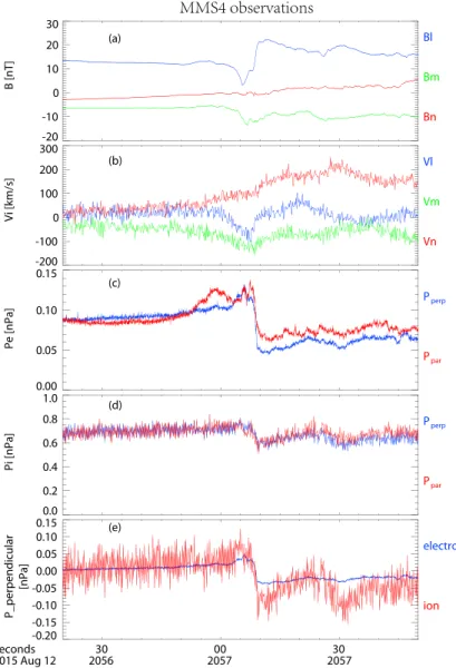
Figure 3a shows the magnetic field of MMS 4 in LMN coordinates. The ion bulk velocity, measured by MMS 4 and presented in Figure 3b, is primarily flowing in N direction, consistent with the DF sitting at the leading edge of the ion bulk flow event. Figures 3c and 3d show the plasma pressure (perpendicular in blue and parallel in red) for electrons and ions, respectively. Figure 3e shows the perpendicular ion (in red) and electron (in blue) pressure detrended by the average value between 20:56:30 UT and 20:57:30 UT. Although the ion pressure is about 1 order of magnitude higher than the electron, the detrended electron pressure shows a comparable decrease to that of the ions across the DF layer. Thus, the pressure gradients are similar, which in turn suggests that the electron diamagnetic current is nonnegligible as compared to the ion diamagnetic current. The currents carried by both ions and electrons are analyzed in the next section.
2.2. Carriers of the Perpendicular Current Associated With DF
In this section, we analyze the carriers of the intense current density associated with this dipolarization front. In ideal magnetohydrodynamics (MHD) theory, the current density can be expressed as equation (2)
J⟂= B B2×𝜌 du dt + B B2× ∇P, (2)
where𝜌 represents the mass density, u is the plasma bulk velocity, B is the magnetic field vector, and P repre-sents the plasma pressure. The first term on the right-hand side (RHS) is the inertial current, which is usually negligible in comparison with the pressure gradient (i.e., the second term on the RHS of equation (2)) in the magnetosphere current system [e.g., Lui, 1996; Shiokawa et al., 1997; Birn et al., 1999]. We do not directly calcu-late the full 3-D pressure gradient since the plasma measurements from MMS 1 were not available. However, the DF is a tangential discontinuity [e.g., Sergeev et al., 2009; Fu et al., 2012b; Liu et al., 2015a], a result which is also supported by our MVA analysis results, demonstrating that this DF is a quasi-1-D structure and Bnwas almost consistent and near 0 across the DF layer. Since we have determined the propagation speed of the DF structure from the constant velocity method applied to the B field data from all four spacecraft, we can thus calculate the pressure gradient in the normal direction from single-spacecraft plasma measurements. In the two-fluid frame, the plasma pressure could be expressed as two contributions from both ions and electrons, respectively, i.e., P = Pi+ Pe. So the m component of the perpendicular current density is expressed as
J⟂m= Bl
Journal of Geophysical Research: Space Physics
10.1002/2016JA023401
Figure 3. Measurements from MMS 4. (a) Magnetic field inLMNcoordinates, (b) the ion bulk velocity inLMN
coordinates, (c and d), the plasma pressure for both electron and ions (the blue and red curves represent the perpendicular and parallel components, respectively), and (e) the perpendicular plasma pressure for both ion and electron, detrended with the average value between 20:56:30 UT and 20:57:30 UT.
The two RHS terms are the ion diamagnetic current and electron diamagnetic current in m direction, respec-tively. We converted time differences to distances 𝜕P
𝜕t = 𝜕Pi,e
𝜕n ⋅ Vnand reconstructed the profile of ∇n(Pi,e). Similarly, we can also calculate the L component diamagnetic current density.
J⟂l= −Bm
B2∇n(Pi+ Pe). (4)
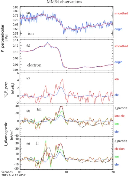
Figures 4a and 4b present the ion and electron perpendicular pressure. The blue curve shows the original data, and the red curve is the smoothed data with a 900 ms window. Figure 4c shows the reconstructed ion (red) and electron (blue) pressure gradient in the normal direction, which is calculated from the smoothed data in Figures 4a and 4b. As we can see from the plots, the smoothed data follow the major trends that we can identify by eye. Figures 4d and 4e show the diamagnetic currents (blue: electron, green: ion, and red: electron + ion), and the black curves are the m and l components of perpendicular current directly calculated from particle distributions. For the m component current, the electron and ion pressure have comparable peak gradients, which contribute current density of ∼ 13 nA/m2and ∼ 24 nA/m2at around 20:57:09 UT, respectively. Hence, the total diamagnetic current has a peak of ∼ 37 nA/m2. Similarly, the peak of L component diamag-netic current is ∼ 30 nA/m2that is contributed by ions of ∼ 18 nA/m2and electrons of ∼ 12 nA/m2. The total diamagnetic currents in both l and m components are highly consistent with the particle measurements.
Figure 4. (a, b) The perpendicular plasma pressure of ions and electrons; the red curves show the smoothed data
(a 900 ms smoothing window) of the original data that are given by the blue curves; (c) the ion (red) and electron (blue) pressure gradient that is calculated by𝜕P
𝜕t ⋅ Vn. (d and e) Thelandmcomponent current densities contributed by
electron (blue) and ion (green) diamagnetic drift. The red curve is the total diamagnetic current, as the sum of both electron and ion diamagnetic currents. The black curves are the current calculated from particle distribution functions.
Figure 5 shows the terms associated with generalized Ohm’s law. Previous discussions on generalized Ohm’s law are mostly associated with the plasma flow [e.g., Lui et al., 2007], which has a scale of a few Earth radii. Usually, spin resolution particle measurements are sufficient for this large-scale investigation. However, on the DF, as the front boundary is usually in a scale of ion gyroradius and can only be measured in one to two spin periods, higher temporal resolution measurements are required to study the generalized Ohm’s law. The high-cadence particle measurements from MMS provide for the first time the high-resolution pressure gradi-ent and bulk velocity for both ions and electrons, which allow the analysis of the generalized Ohm’s law within the DF with the necessary temporal cadence. Figures 5a–5c show the three components of both E + Vi× B andJ×Bne terms in LMN coordinates. The electric field E, ion bulk velocity Vi, magnetic field B, current density J, and number density n are directly from MMS 4 measurements. For both the E + Vi× B andJ×B
ne terms, the Ncomponent is the dominant component, while both L and M components are relatively small, although there were high-amplitude spikes in the m component that remain poorly understood. For the major com-ponent, i.e., the N comcom-ponent, a clear divergence exists between these two terms (between 20:57:08 UT and 20:57:10 UT), which directly implies that Hall MHD is not suitable in this DF structure.
Journal of Geophysical Research: Space Physics
10.1002/2016JA023401
Figure 5. A breakdown of the individual terms in the generalized Ohm’s law. (a–c)L,M, andNcomponents ofE + Vi× B
andJ×B
ne and (d) theNcomponent ofE + Ve× B,E + Vi× B − J×B
ne and− ∇Pe
ne terms.
Figure 5d presents the N component of the −∇Pe
ne, E + Ve× B, and E + Vi× B − J×B
ne. As expected, E + Ve× B and E + Vi× B − J×B
ne are exactly the same, which is, however, slightly greater than − ∇Pe
ne . We believe the small difference between −∇Pe
ne and E + Ve× B is caused by the uncertainty in electric field measurements. The uncertainties from electric field measurements affect the accuracy of E × B drift which, in turn, produces uncertainties in calculated bulk ion and electron velocities. However, this uncertainty does not affect the total current density, as this E × B drift velocity is the same for both ions and electrons and, hence, is canceled. In order to demonstrate that both measurements are reliable, we present the total diamagnetic current den-sity and the current denden-sity derived from particle distribution functions (Figures 4d and 4e). Both the total diamagnetic and particle-derived currents are consistent, demonstrating that the particle measurements are indeed reliable.
3. Discussion and Conclusions
In this paper, we study a dipolarization front (DF) using the high temporal plasma and field measurements from MMS on 12 August 2015. We analyzed the current carriers and validity of the electron frozen-in condition
for the DF, using these high temporal cadence measurements. The variations of plasma moments (derived from the 3-D particle distributions) within a DF are the first directly presented using MMS high-cadence mea-surements. Using both minimum variance analysis (MVA) and minimum directional derivation (MDD) analysis, we find that the DF structure is a quasi-1-D structure that in this case propagates with a speed of ∼ 150 km s−1 toward the midnight near-Earth magnetotail. Schmid et al. [2016] clearly demonstrate that the x component of propagation speed becomes much smaller in dawnside/duskside than the midnightside, and in our event, the DF was observed at very duskside, so the propagation was mostly in YZ direction. The ion gyroradius is 800 km for energy at 7 keV (the ion temperature, not shown here) in B ∼ 15 nT environment, and the duration of the DF is ∼ 4 s, corresponding to a spatial scale of ∼ 600 km, which is comparable to one ion gyroradius, so we would not expect ideal MHD to hold on DF structure.
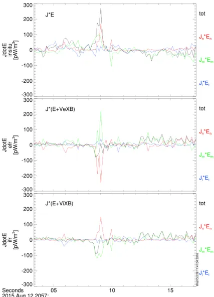
The new experimental capabilities provided by MMS and discussed above allow us to address the fundamen-tal question about the role of DFs in energy conversion in the magnetotail. Previous studies have reported that energy is transferred from field to plasma (i.e., J⋅ E >0) on the DF [Hamrin et al., 2013; Huang et al., 2015]. However, the accuracy of J⋅ E strongly depends on the current density calculation and 3-D electric field mea-surements. We note that both are significantly improved over previous missions by using the unprecedented temporal and spatial measurements available from MMS measurements. Moreover, we specifically point out that it is essential to calculate the Joule heating term in the structure’s rest frame, i.e., in a frame that is moving with magnetic structure, as described in Paschmann et al. [1979]. The energy transfer from the electromag-netic field to plasmas in plasma rest frame is formulated as a Lorentz-invariant scalar quantity [Zenitani et al., 2011]. It is certainly difficult to obtain the moving speed of magnetic field from in situ measurements, but pre-vious research typically uses ion bulk velocity or electron bulk velocity in the calculation, i.e., J⋅ (E + Vi× B) or J⋅ (E + Ve× B). It is interesting to note that the current literature refer to Joule heating as J⋅ E [e.g., Zong
et al., 2007; Hamrin et al., 2013; Huang et al., 2015], J⋅ (E + Vi× B) [e.g., Runov et al., 2011a; Angelopoulos et al., 2013], and J⋅ (E + Ve× B) [e.g., Zenitani et al., 2011; Burch et al., 2016b], and we can directly calculate all three versions below. Figure 6 shows the results from the three different calculations with measurements from MMS 4. Clearly, J⋅ E is positive, with a peak power of ∼ 250 pW/m3. The positive value is consistent with previous energy conversion on the DF with J⋅ E [e.g., Huang et al., 2015]. J ⋅ (E + Ve× B) and J⋅ (E + Vi× B) are both negative, with a peak power of ∼ −80 pW/m3. If one wishes to compute pure dissipation excluding bulk fluid acceleration, then one calculates the electric field in the rest frame of the fluid [Birn and Hesse, 2005; Fu et al., 2016]. This follows from the fact that J⋅ (V × B) = −V ⋅ (J × B), i.e., this term represents the work done by the Lorentz force on the fluid. Note that whether this is done in the electron (V = Ve) or ion (V = Vi) frame does not matter because the V × B terms are different by −neJ which gives zero contribution to energy conversion (J⋅ (J × B) = 0). This gives the potential mathematical reason as to why the calculations in both electron and ion rest frame (Figure 6) are consistent and hence this consistency can also serve as a cross validation of our calculation that plasma energy is being converted to fields in our event.
The current density associated with DFs is usually derived from the curlometer method applied to four-point magnetic field measurements, i.e., from Cluster and MMS tetrahedrons. However, in the derivation of the field-aligned current within a tetrahedron, the accuracy has been shown to depend on the consistency of the magnetic field direction at the four points, as indicated by Yao et al. [2016]. Particularly in the magnetic dip region immediately ahead of the DF, the magnetic field strength is usually small, and the direction of magnetic field is thus subject to large potential variation. The previous tetrahedron measurements from Cluster pro-vided their smallest interspacecraft separation in 2003 magnetotail season, which was ∼ 200 km. As shown in
Yao et al. [2016], the magnetic field directions of the four spacecraft are usually very different in the magnetic
dip region. The separation of the MMS tetrahedron is significantly smaller than the Cluster tetrahedron, which thus provides a much more accurate calculation for small-scale field-aligned current densities, as evidenced by a much smaller CMD index as highlighted by Yao et al. [2016]. We note here that the importance of CMD parameter is not only essential in determining the accuracy of FACs but also important in other calculations from the tetrahedron measurements (e.g., the calculation of Hall term J × B).
It is very interesting that the electron diamagnetic current density is about 30% of the total current density, which is significantly smaller than the conclusion in Zhang et al. [2011], which concluded that electrons con-tribute up to 60% of the total current density. The remainder of the current density (40%) was suggested to be contributed by polarization currents generated by dynamic pressure gradient. However, in our paper, we found a very good consistency between currents calculated from particle and magnetic field (Figures 4d and 4e), which directly demonstrates that the thermal pressure contribution is much more significant than
Journal of Geophysical Research: Space Physics
10.1002/2016JA023401
Figure 6. Three methods of Joule heating calculation, i.e.,J⋅ E + Ve× BandJ⋅ E + Vi× B. The blue, green, and red curves represent the three component contributions, and the black curves give the total values.
the dynamic pressure. Moreover, the total current density (from particle or curlometer) can be fully explained by the sum of electron and ion diamagnetic currents. Although we do not exclude the potential importance of the dynamic pressure gradients for the current density generation, our analyses clearly show that for this event the total diamagnetic currents constitute the majority of the currents within the DF.
With the more accurate measurement of current density and electric field from MMS, we can also determine the generalized Ohm’s law on the DF. Our results show direct evidence of the violation of ion frozen condition, as one should naturally expect since the DF has a scale of ion gyroradius. Moreover, we show a general con-sistency of −∇Pe
ne and E + Vi× B − J×B
ne terms but cannot conclude that E + Vi× B − J×B
ne = − ∇Pe
ne on a one-to-one basis with these data. It is very likely that EMHD holds on the DF layer, while it is necessary to present more events from the MMS tetrahedron with a smaller spatial separation in the future. In previous studies of Ohm’s law on the DF [e.g., Fu et al., 2012b], the high-resolution electron pressure was derived by interpolating the spin resolution temperature to high resolution on the DF, which is only valid when the temperature does not significantly change across the DF. The electron pressure in this present paper is directly calculated at a resolu-tion of 30 ms. Moreover, we found that the decrease of electron pressure on the DF was not only contributed by the decrease in number density but also by a significant decrease in temperature (not shown in the present paper), which suggests that the assumption for interpolating temperature to high-resolution data is insuffi-cient. The cross validation amongst −∇Pene, E + Vi× B −
J×B
ne, and E + Ve× B provides strong supports to our conclusion. We have also noted that the electron temperature at the DF is slightly anisotropic, which may
modify the diamagnetic current density carried by electrons in our calculation. It is worthy of a further study on the anisotropy effect on the DF when measurements are available from all four spacecraft, although the electron anisotropy behind DF has been comprehensively discussed in previous papers [Fu et al., 2011, 2012a;
Runov et al., 2013; Tang et al., 2016]. In this study, we do not discuss the effect on current density from electron
anisotropy behind the DF, as this effect also strongly depends on the radius of magnetic curvature, which is up to ∼ 0.7 REbehind the DF [Li et al., 2011]. The separation of MMS is thus too small to study this effect. We suggest that a proper analysis with Cluster tetrahedron on this effect would be ideal. In addition, the good consistency between the diamagnetic current (ions + electrons) and the current density directly integrated from particle distributions suggests that the anisotropy current on the DF in our event is not important. In this paper, we presented a single case that was observed in the duskside of the magnetotail. It is still very important to analyze more events with MMS data, especially the DF events near the midnight sector of the magnetotail after the mission apogee processes into this region the magnetosphere during summer season of 2016. However, the FPI instruments were not operated with burst mode, meaning that the high-cadence particle distribution in magnetotail region is still very little; our event is one of very few events that could reveal the dynamics within a kinetic magnetic structure, such as a DF. Further comparisons between DFs observed in midnight and dawnside/duskside would provide a better understanding of the relations between the DF and magnetotail reconnection, as well as how DFs impact magnetotail dynamics on a statistical basis. Our main results are summarized below:
1. Using high temporal particle measurements from MMS, we revisit the current carriers and generalized Ohm’s law on dipolarization fronts and provide a direct examination of the assumptions applied in previous research with Cluster and THEMIS measurements.
2. Although the ion pressure is about 1 order of magnitude higher than that of the electron, the electron pres-sure gradient is of the same order as the ion prespres-sure gradient. Hence, we show for the first time that the diamagnetic current carried by electrons is about 60% of that carried by ions. We calculate the current from the curlometer, directly integrate from particle distribution functions, and found that the three calcula-tions are highly consistent, which demonstrates that the polarization current in our event is not important, and the total perpendicular current density on DF can be fully explained by diamagnetic drifts of ions and electrons.
3. On the dipolarization front itself, the ion frozen-in condition is clearly broken, since the magnetic field dra-matically changes over the scale of an ion gyroradius. Our result shows that E + Ve× B≠ 0 on the DF such that assumptions of Hall MHD do not hold. We find a general consistency of E + Vi× B −
J×B ne = −
∇Pe ne, so it is very likely that electron frozen-in condition still holds on the DF.
4. Energy is being converted from plasma to fields in our event, although similar results have been previously explained as an opposite energy conversion only based on the directly measured J⋅ E >0.
References
Angelopoulos, V., A. Runov, X.-Z. Zhou, D. Turner, S. Kiehas, S.-S. Li, and I. Shinohara (2013), Electromagnetic energy conversion at reconnection fronts, Science, 341(6153), 1478–1482.
Balikhin, M., A. Runov, S. Walker, M. Gedalin, I. Dandouras, Y. Hobara, and A. Fazakerley (2014), On the fine structure of dipolarization fronts,
J. Geophys. Res. Space Physics, 119(8), 6367–6385, doi:10.1002/2014JA019908.
Birn, J., and M. Hesse (2005), Energy release and conversion by reconnection in the magnetotail, Ann. Geophys., 23, 3365–3373. Birn, J., M. Hesse, G. Haerendel, W. Baumjohann, and K. Shiokawa (1999), Flow braking and the substorm current wedge, J. Geophys. Res.,
104(A9), 19,895–19,903.
Burch, J., T. Moore, R. Torbert, and B. Giles (2016a), Magnetospheric multiscale overview and science objectives, Space Sci. Rev., 199(1–4), 5–21.
Burch, J., et al. (2016b), Electron-scale measurements of magnetic reconnection in space, Science, 352(6290), AAF2939.
Dunlop, M., D. Southwood, K.-H. Glassmeier, and F. Neubauer (1988), Analysis of multipoint magnetometer data, Adv. Space Res., 8(9), 273–277.
Ergun, R., et al. (2016), The axial double probe and fields signal processing for the MMS mission, Space Sci. Rev., 199(1–4), 167–188. Fu, H. S., Y. V. Khotyaintsev, M. André, and A. Vaivads (2011), Fermi and betatron acceleration of suprathermal electrons behind
dipolarization fronts, Geophys. Res. Lett., 38, L16104, doi:10.1029/2011GL048528.
Fu, H. S., Y. Khotyaintsev, A. Vaivads, M. André, V. Sergeev, S. Huang, E. Kronberg, and P. Daly (2012a), Pitch angle distribution of suprathermal electrons behind dipolarization fronts: A statistical overview, J. Geophys. Res., 117, A12221, doi:10.1029/2012JA018141. Fu, H. S., Y. V. Khotyaintsev, A. Vaivads, M. André, and S. Huang (2012b), Electric structure of dipolarization front at sub-proton scale,
Geophys. Res. Lett., 39, L06105, doi:10.1029/2012GL051274.
Fu, H. S., A. Vaivads, Y. V. Khotyaintsev, M. André, J. Cao, V. Olshevsky, J. Eastwood, and Retinò (2016), Intermittent energy dissipation by turbulent reconnection, Geophys. Res. Lett., 44, 37–43, doi:10.1002/2016GL071787.
Hamrin, M., et al. (2013), The evolution of flux pileup regions in the plasma sheet: Cluster observations, J. Geophys. Res. Space Physics,
118(10), 6279–6290, doi:10.1002/jgra.50603.
Acknowledgments
MMS data sets were provided by the MMS science working group teams through the link (http://lasp.colorado. edu/mms/sdc/about/browse/). Z.Y., A.N.F., I.J.R., and C.J.O. are supported by UK Science and Technology Facilities Council (STFC) grant (ST/L005638/1) at UCL/MSSL. Z.Y. is a Marie-Curie COFUND postdoctoral fellow at the University of Liege, cofunded by the European Union. I.J.R. is also supported by STFC grant (ST/L000563/1) and National Environmental Research Council (NERC) grant (NE/L007495/1). C.W. is supported by STFC grant ST/M000885/1. A.N.F., I.J.R., and C.J.O. are currently funded via the MSSL consolidated grant ST/N000722/1. This work is also supported by NSFC grant (41404117).
Journal of Geophysical Research: Space Physics
10.1002/2016JA023401
Henderson, P., C. Owen, A. Lahiff, I. Alexeev, A. Fazakerley, E. Lucek, and H. Reme (2006), Cluster peace observations of electron pressure tensor divergence in the magnetotail, Geophys. Res. Lett., 33, L22106, doi:10.1029/2006GL027868.
Hoffman, R., M. Sugiura, and N. Maynard (1985), Current carriers for the field-aligned current system, Adv. Space Res., 5(4), 109–126. Huang, S., et al. (2015), Electromagnetic energy conversion at dipolarization fronts: Multispacecraft results, J. Geophys. Res. Space Physics,
120(6), 4496–4502.
Hwang, K.-J., M. L. Goldstein, E. Lee, and J. S. Pickett (2011), Cluster observations of multiple dipolarization fronts, J. Geophys. Res., 116, A00I32, doi:10.1029/2010JA015742.
Li, S.-S., V. Angelopoulos, A. Runov, X.-Z. Zhou, J. McFadden, D. Larson, J. Bonnell, and U. Auster (2011), On the force balance around dipolarization fronts within bursty bulk flows, J. Geophys. Res., 116(A00I35), doi:10.1029/2010JA015884.
Lindqvist, P.-A., et al. (2016), The spin-plane double probe electric field instrument for MMS, Space Sci. Rev., 199(1–4), 137–165. Liu, J., V. Angelopoulos, A. Runov, and X.-Z. Zhou (2013a), On the current sheets surrounding dipolarizing flux bundles in the magnetotail:
The case for wedgelets, J. Geophys. Res. Space Physics, 118, 2000–2020, doi:10.1002/jgra.50092.
Liu, J., V. Angelopoulos, X.-Z. Zhou, A. Runov, and Z. Yao (2013b), On the role of pressure and flow perturbations around dipolarizing flux bundles, J. Geophys. Res. Space Physics, 118, 7104–7118, doi:10.1002/2013JA019256.
Liu, J., V. Angelopoulos, X.-Z. Zhou, Z.-H. Yao, and A. Runov (2015a), Cross-tail expansion of dipolarizing flux bundles, J. Geophys. Res. Space
Physics, 120, 2516–2530, doi:10.1002/2015JA020997.
Liu, J., V. Angelopoulos, X. Chu, X.-Z. Zhou, and C. Yue (2015b), Substorm current wedge composition by wedgelets, Geophys. Res. Lett., 42(6), 1669–1676, doi:10.1002/2015GL063289.
Lu, S., A. Artemyev, V. Angelopoulos, Q. Lu, and J. Liu (2016), On the current density reduction ahead of dipolarization fronts, J. Geophys. Res.
Space Physics, 121, 4269–4278, doi:10.1002/2016JA022754.
Lui, A. (1996), Current disruption in the Earth’s magnetosphere: Observations and models, J. Geophys. Res., 101(A6), 13,067–13,088. Lui, A. (2015), Dipolarization fronts and magnetic flux transport, Geosci. Lett., 2(1), 1.
Lui, A., Y. Zheng, H. Reme, M. Dunlop, G. Gustafsson, and C. Owen (2007), Breakdown of the frozen-in condition in the Earth’s magnetotail,
J. Geophys. Res., 112, A04215, doi:10.1029/2006JA012000.
Mauk, B., et al. (2016), The energetic particle detector (EPD) investigation and the energetic ion spectrometer (EIS) for the magnetospheric multiscale (MMS) mission, Space Sci. Rev., 199(1–4), 471–514.
McPherron, R., C. Russell, M. Kivelson, and P. Coleman (1973), Substorms in space: The correlation between ground and satellite observations of the magnetic field, Radio Sci., 8(11), 1059–1076.
Nakamura, R., et al. (2002), Motion of the dipolarization front during a flow burst event observed by Cluster, Geophys. Res. Lett., 29(20), 3–1, doi:10.1029/2002GL015763.
Nakamura, R., et al. (2009), Evolution of dipolarization in the near-Earth current sheet induced by earthward rapid flux transport,
Ann. Geophys., 27(4), 1743–1754, doi:10.5194/angeo-27-1743-2009.
Palin, L., C. Jacquey, J.-A. Sauvaud, B. Lavraud, E. Budnik, V. Angelopoulos, U. Auster, J. P. McFadden, and D. Larson (2012), Statistical analysis of dipolarizations using spacecraft closely separated alongzin the near-Earth magnetotail, J. Geophys. Res., 117, A09215, doi:10.1029/2012JA017532.
Panov, E., et al. (2010), Multiple overshoot and rebound of a bursty bulk flow, Geophys. Res. Lett., 37, L08103, doi:10.1029/2009GL041971. Panov, E., W. Baumjohann, M. Kubyshkina, R. Nakamura, V. Sergeev, V. Angelopoulos, K.-H. Glassmeier, and A. Petrukovich (2014), On the increasing oscillation period of flows at the tailward retreating flux pileup region during dipolarization, J. Geophys. Res. Space Physics,
119(8), 6603–6611, doi:10.1002/2014JA020322.
Paschmann, G., et al. (1979), Plasma acceleration at the Earth’s magnetopause—Evidence for reconnection, Nature, 282, 243–246. Pollock, C., et al. (2016), Fast plasma investigation for magnetospheric multiscale, Space Sci. Rev., 199(1-4), 331–406.
Pritchett, P., and F. Coroniti (2013), Structure and consequences of the kinetic ballooning/interchange instability in the magnetotail,
J. Geophys. Res. Space Physics, 118(1), 146–159, doi:10.1029/2012JA018143.
Robert, P., M. W. Dunlop, A. Roux, and G. Chanteur (1998), Accuracy of current density determination, in Analysis Methods for Multi-spacecraft
Data, vol. 398, pp. 395–418, ISSI Scientific Reports Series, SR-001, Kluwer Acad., Bern.
Runov, A., V. Angelopoulos, X.-Z. Zhou, X.-J. Zhang, S. Li, F. Plaschke, and J. Bonnell (2011a), A THEMIS multicase study of dipolarization fronts in the magnetotail plasma sheet, J. Geophys. Res., 116, A05216, doi:10.1029/2010JA016316.
Runov, A., et al. (2011b), Dipolarization fronts in the magnetotail plasma sheet, Planet. Space Sci., 59(7), 517–525.
Runov, A., V. Angelopoulos, C. Gabrielse, X.-Z. Zhou, D. Turner, and F. Plaschke (2013), Electron fluxes and pitch-angle distributions at dipolarization fronts: THEMIS multipoint observations, J. Geophys. Res. Space Physics, 118(2), 744–755, doi:10.1002/jgra.50121. Russell, C., J. Gosling, R. Zwickl, and E. Smith (1983), Multiple spacecraft observations of interplanetary shocks: ISEE three-dimensional
plasma measurements, J. Geophys. Res., 88(A12), 9941–9947.
Russell, C., et al. (2016), The magnetospheric multiscale magnetometers, Space Sci. Rev., 199(1–4), 189–256.
Schmid, D., M. Volwerk, R. Nakamura, W. Baumjohann, and M. Heyn (2011), A statistical and event study of magnetotail dipolarization fronts,
Ann. Geophys., 29, 1537–1547.
Schmid, D., et al. (2016), A comparative study of dipolarization fronts at MMS and Cluster, Geophys. Res. Lett., 43, 6012–6019, doi:10.1002/2016GL069520.
Sergeev, V., V. Angelopoulos, S. Apatenkov, J. Bonnell, R. Ergun, R. Nakamura, J. McFadden, D. Larson, and A. Runov (2009), Kinetic structure of the sharp injection/dipolarization front in the flow-braking region, Geophys. Res. Lett., 36, L21105, doi:10.1029/2009GL040658. Shi, Q., C. Shen, Z. Pu, M. Dunlop, Q.-G. Zong, H. Zhang, C. Xiao, Z. Liu, and A. Balogh (2005), Dimensional analysis of observed structures
using multipoint magnetic field measurements: Application to Cluster, Geophys. Res. Lett., 32, L12105, doi:10.1029/2005GL022454. Shi, Q., C. Shen, M. Dunlop, Z. Pu, Q.-G. Zong, Z. Liu, E. Lucek, and A. Balogh (2006), Motion of observed structures calculated from
multi-point magnetic field measurements: Application to Cluster, Geophys. Res. Lett., 33, L08109, doi:10.1029/2005GL025073. Shiokawa, K., W. Baumjohann, and G. Haerendel (1997), Braking of high-speed flows in the near-Earth tail, Geophys. Res. Lett., 24(10),
1179–1182.
Shiokawa, K., Y. Miyashita, I. Shinohara, and A. Matsuoka (2005), Decrease inBzprior to the dipolarization in the near-Earth plasma sheet,
J. Geophys. Res., 110, A09219, doi:10.1029/2005JA011144.
Sitnov, M., M. Swisdak, and A. Divin (2009), Dipolarization fronts as a signature of transient reconnection in the magnetotail, J. Geophys. Res.,
114, A04202, doi:10.1029/2008JA013980.
Sitnov, M., N. Buzulukova, M. Swisdak, V. Merkin, and T. Moore (2013), Spontaneous formation of dipolarization fronts and reconnection onset in the magnetotail, Geophys. Res. Lett., 40, 22–27, doi:10.1029/2012GL054701.
Sitnov, M., V. Merkin, M. Swisdak, T. Motoba, N. Buzulukova, T. Moore, B. Mauk, and S. Ohtani (2014), Magnetic reconnection, buoyancy, and flapping motions in magnetotail explosions, J. Geophys. Res. Space Physics, 119(9), 7151–7168, doi:10.1002/2014JA020205.
Sonnerup, B., and L. Cahill (1967), Magnetopause structure and attitude from Explorer 12 observations, J. Geophys. Res., 72(1), 171–183. Sonnerup, B. U., and M. Scheible (1998), Minimum and maximum variance analysis, in Analysis Methods for Multi-spacecraft Data, edited by
G. Paschmann and P. W. Daly, pp. 185–220, ISSI SR-001, ESA Publ. Div., Noordwijk, Netherlands.
Sun, W., et al. (2013), Field-aligned currents associated with dipolarization fronts, Geophys. Res. Lett., 40(17), 4503–4508, doi:10.1002/grl.50902.
Tang, C., M. Zhou, Z. Yao, and F. Shi (2016), Electron acceleration associated with the magnetic flux pileup regions in the near-Earth plasma sheet: A multicase study, J. Geophys. Res. Space Physics, 121, 4331–4342, doi:10.1002/2016JA022406.
Torbert, R., et al. (2016a), Estimates of terms in Ohm’s law during an encounter with an electron diffusion region, Geophys. Res. Lett., 43, 5918–5925, doi:10.1002/2016GL069553.
Torbert, R., et al. (2016b), The FIELDS instrument suite on MMS: Scientific objectives, measurements, and data products, Space Sci. Rev.,
199(1–4), 105–135.
Yao, Z., et al. (2012), Mechanism of substorm current wedge formation: THEMIS observations, Geophys. Res. Lett., 39, L13102, doi:10.1029/2012GL052055.
Yao, Z., et al. (2013), Current structures associated with dipolarization fronts, J. Geophys. Res. Space Physics, 118(11), 6980–6985, doi:10.1002/2013JA019290.
Yao, Z., et al. (2014), Current reduction in a pseudo-breakup event: THEMIS observations, J. Geophys. Res. Space Physics, 119(10), 8178–8187, doi:10.1002/2014JA020186.
Yao, Z., et al. (2016), Substructures within a dipolarization front revealed by high-temporal resolution Cluster observations, J. Geophys. Res.
Space Physics, 121, 5185–5202, doi:10.1002/2015JA022238.
Yao, Z. H., et al. (2015), A physical explanation for the magnetic decrease ahead of dipolarization fronts, Ann. Geophys., 33(10), 1301–1309, doi:10.5194/angeo-33-1301-2015.
Zenitani, S., M. Hesse, A. Klimas, and M. Kuznetsova (2011), New measure of the dissipation region in collisionless magnetic reconnection,
Phys. Rev. Lett., 106(19), 195003.
Zhang, X.-J., V. Angelopoulos, A. Runov, X.-Z. Zhou, J. Bonnell, J. McFadden, D. Larson, and U. Auster (2011), Current carriers near dipolarization fronts in the magnetotail: A THEMIS event study, J. Geophys. Res., 116, A00I20, doi:10.1029/2010JA015885.
Zhou, M., et al. (2013), Cluster observations of kinetic structures and electron acceleration within a dynamic plasma bubble, J. Geophys. Res.
Space Physics, 118(2), 674–684, doi:10.1029/2012JA018323.
Zong, Q.-G., et al. (2007), Earthward flowing plasmoid: Structure and its related ionospheric signature, J. Geophys. Res., 112, A07203, doi:10.1029/2006JA012112.