T
T
H
H
È
È
S
S
E
E
En vue de l'obtention du
D
D
O
O
C
C
T
T
O
O
R
R
A
A
T
T
D
D
E
E
L
L
’
’
U
U
N
N
I
I
V
V
E
E
R
R
S
S
I
I
T
T
É
É
D
D
E
E
T
T
O
O
U
U
L
L
O
O
U
U
S
S
E
E
Délivré par l’Université Paul Sabatier III Discipline ou spécialité : Chimie-Océanographie
JURY
V. Garçon – Directrice de Recherches, CNRS, LEGOS, Toulouse, France M. Comtat – Professeur, Université Paul Sabatier Toulouse III, France
D. Connelly – Senior Research Scientist, National Oceanography Center, Royaume-Uni G. W. Luther III – Professeur, Université de Delaware, États-Unis
J.-L. Marty – Professeur, Université de Perpignan, France N. P. Revsbech – Professeur, Université d’Aarhus, Danemark M. Trojanowicz – Professeur, Université de Varsovie, Pologne
Ecole doctorale : SDU2E
Unité de recherche : Laboratoire d’Etudes en Géophysique et Océanographie Spatiales Directeur(s) de Thèse : Véronique Garçon
Co-directeur de Thèse : Maurice Comtat
Présentée et soutenue par
Justyna Elżbieta Jońca
Le 1 Octobre 2012Titre : Méthodes électrochimiques pour la surveillance autonome des espèces chimiques (oxygène et phosphate) dans l’eau de mer :
I dedicate this work to my beloved mother.
Acknowledgments
Working on the Ph.D. has been a wonderful experience. It is hard to say whether it has been grappling with the topic itself which has been the real learning experience, or grappling with how to write papers, give talks, work in a group, and stay focussed to the late night hours...In any case, I am indebted to many people for making the time working on my Ph.D. an unforgettable experience.
First of all, I am deeply grateful to my advisor Véronique Garçon for introducing me into the fascinating world of oceanography. Working with her has been a real pleasure to me. She has oriented and supported me with care, and has always been patient and encouraging in times of new ideas and difficulties. Her ability to select and approach compelling research problems, her high scientific standards, and her hard work set an example. Despite many responsibilities, she always had a moment to correct my manuscripts and prepare me for conferences. Above all, she made me feel friend, which I appreciate from my heart.
I will forever be thankful to my co-advisor Maurice Comtat for his scientific advice and knowledge and many insightful discussions and suggestions. He was my primary resource for getting my electrochemical questions answered. I am also grateful for our long discussions about french cooking and wines.
I also thank my scientific advisor Niels Peter Revsbech from Aarhus University in Denmark for choosing a very interesting topic for my secondment in his laboratory and for helping me achieve excellent results in a very short period of time.
I also have to thank the members of my PhD committee: George Luther III, Douglas
Connelly, Niels Peter Revsbech, Marek Trojanowicz and Jean-Louis Marty for their
helpful suggestions and hard questions. Thank you all for having accepted this additional work.
During my PhD studies I was supported by an Initial Training Network Marie Curie within the SENSEnet project (grant agreement N° 237868). The SENSEnet project gave me this tremendous opportunity to collaborate with research institutes across Europe and to work with the best scientists within the marine chemistry science. I will be forever grateful for all SENSEnet meetings, field courses and other workshops full of scientific discussions and presentations. All that was possible thanks to an excellent project management and I have to thank for that Carla Sands and Douglas Connelly. In this place I would like to thank also all SENSEnet students for effective brainstorming during our workshops and for great time we had together during informal meetings.
were crucial in my work and for her constant dialogue with me in french which forced me to learn french faster. I would like to thank Carole Barus, William Giraud, Ludovic Lesven and Margeaux Gourdal for all scientific and non-scientific discussions. I thank Nicolas
Striebig and Marcel Belot for designing and manufacturing my measurement
electrochemical cell. Many thanks to Aurélien Paulmier for sharing with me his huge knowledge on Peruvian waters and for his help in preparing the oceanographic cruise offshore Peru in October 2010. In this place I would like to also thank officers, scientists and crew of Pelagico 1011-12-BIC OLAYA cruise aboard R/V Jose Olaya Balandra for their assistance in the collection of water samples and to IMARPE laboratory for organization of the cruise.
I would also like to thank the administrative staff from the laboratory (Nadine,
Martine, Brigitte) for their so precious help.
I thank my family because I would not have gone so far without them. I wished my mum had lived longer for my graduation. She sacrificed her life for my sister and brothers and myself and provided unconditional love and care. The memory of her will be with me for the rest of my life. Special thanks to my sister Agnieszka, my brothers Krzysztof and Piotr for being supportive when times were rough and for long phone conversations about everything and nothing.
I thank my best friend Agata for having faith in me and my intellect and for our long “intelligent” discussions on Skype. Finally, I would like to thank my boyfriend and soul-mate
Wojtek for sharing with me the passion for science and for his love and support during my
SUMMARY
General introduction 11
Introduction générale (français) 15
CHAPTER I: Introduction on ocean biogeochemistry
and on Oxygen Minimum Zones 19
1. Introduction on ocean biogeochemistry 21
1.1. The role of ocean in the global carbon cycle 21
1.1.1. The physical and biological carbon pumps 24
1.1.2. Human impact on ocean CO2 uptake 27
1.1.3. Oceanic circulation and global warming 28
1.2. The components of the biological carbon pump 29
1.2.1. Phytoplankton and primary production 29
1.2.2. Role of nutrients and iron in the biological carbon pump 32
1.3. The phosphate in the ocean 33
1.3.1. Chemistry of phosphate 33
1.3.2. The cycle of phosphate in the ocean 34
2. Introduction on Oxygen Minimum Zones (OMZs) 38
2.1. Oxygen in the ocean 38
2.2. Formation, distribution and stability of OMZ 40
2.3. The role of OMZ in the global climate change 42
2.3.1. Influence of OMZ on the biogeochemical cycles
and greenhouse gases budget 42
2.3.2. Biotic response to OMZ 43
3. Summary 44
CHAPTER II: Fundamentals of electrochemical techniques 47
1. Basic concepts 49
1.1. Electrolytes and the electrode-solution interface 49
1.2. The electrode reactions 50
1.3. Galvanic cell and Nernst equation 51
1.4. Electrolysis cell and non-equilibrium processes 53
1.5. Electrochemical methods and apparatus 53
2. Electrochemical kinetics 56
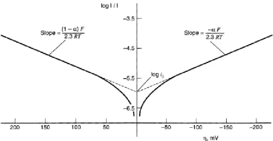
2.1. Faraday’s law and Butler-Volmer’s law 57
2.2. Fick’s diffusion law 60
2.2.1. First case: transport by pure diffusion 61
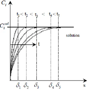
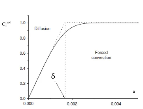
2.2.2. Second case: transport by convective diffusion 63
3. Electrochemical methods used in this work 64
3.1. Diffusion controlled methods: Cyclic voltammetry 64
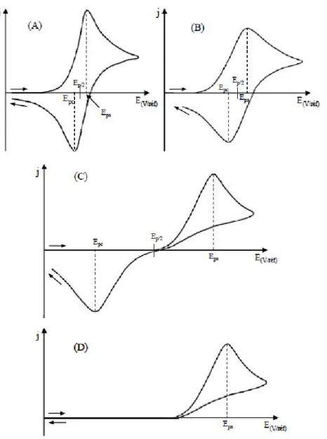
3.1.1. First case: reversible system 66
3.1.2. Second case: irreversible system 67
3.1.3. Third case: quasi-reversible system 67
3.2. Modulated voltammetric techniques-differential pulse voltammetry 67
3.3. Methods controlled by forced convection: hydrodynamic methods 69
3.3.1. Levich’s equation 70
3.3.2. Koutecky-Levich’s equation 70
5.1. CrEr mechanism 74
5.2. ErCi mechanism 75
6. Summary 76
CHAPTER III: In situ phosphate and oxygen monitoring 79
1. Ocean observing systems 81
2. Sensor characteristics for long term ocean monitoring 84
3. Sensors for oxygen in situ measurements 85
3.1. Clark-type oxygen microsensors 89
3.1.1. Construction and functioning 89
3.1.2. Characteristics of Clark-type sensors 91
3.2. STOX sensor as an improved Clark-type sensor 93
3.2.1. Construction and principle of functioning 94
3.2.2. Sensor characteristic 95
3.2.3. In situ applications of STOX sensor 96
3.2.4. Advantages and disadvantages 99
3.3. Optical vs amperometric microsensors 100
4. Methods for phosphate monitoring in seawater 102
4.1. Autonomous phosphate analyzers based on wet chemistry and spectrophotometry 102
4.1.1. Principle of phosphate measurements 102
4.1.2. ANAIS-Autonomous Nutrient Analyzer In Situ 104
4.1.3. Other spectrophotometric analyzers 107
4.2. Alternative phosphate sensing techniques 110
5. Corrosion and biofouling problems 113
6. Summary 114
CHAPTER IV: Improvement of the STOX sensor for
ultra-low oxygen concentrations 117
1. Introduction 119
2. Sensors preparation 120
3. Results and discussion 122
3.1. Optimization of gold plating on silicon membrane 122
3.2. Comparison of traditional and improved STOX sensor 123
3.2.1. Calibration curves and sensitivity 123
3.2.2. Signal stability 124
3.2.3. Detection limit 126
3.2.4. Temperature dependence 126
3.2.5. Response time 128
4. Conclusions and perspectives 129
CHAPTER V: Elucidation of molybdates’ complex chemistry 131
Article 1: Jońca, J., Barus, C., Giraud, W., Thouron, D., Garçon, V., Comtat, M, 2012,
Electrochemical Behaviour of Isopoly- and Heteropolyoxomolybdates Formed During Anodic Oxidation of Molybdenum in Seawater, International Journal of Electrochemical Sciences,
7,7325-7348 133
CHAPTER VI: Electrochemical methods for phosphate detection in seawater 161
Article 2: Jońca, J., Leon-Fernandez, V., Thouron, D., Paulmier, A., Graco, M., Garçon, V.,
2011, Phosphate determination in seawater: Towards an autonomous electrochemical
method, Talanta 87, 161-167 163
Article 3: Jońca, J., Giraud, W., Barus, C., Comtat, M., Striebig, N., Thouron, D., Garçon, V.,
2013, Reagentless and silicate interference free electrochemical phosphate detection in
seawater, Electrochimica acta, 88, 165-169 173
Summary of Articles 2 and 3 181
CHAPTER VII: Analysis of water masses offshore Peru 185
1. Pelagico 1011-12-BIC OLAYA cruise offshore Peru 187 2. Mean circulation in the Oxygen Minimum Zone of the Eastern South Pacific 188
3. Description of waters masses offshore Peru 192
4. The source of relative phosphate minimum on the vertical profiles 198
4.1. Alongshore recirculation of subantarctic waters 198
4.2. Complex biogeochemistry offshore Peru 200
5. Conclusions and perspectives 204
General conclusions 207
Conclusion générale (français) 211
Annexe: 215
Article 4: Giraud, W., Lesven, L., Jońca, J., Barus, C., Gourdal, M., Thouron, D., Garçon, V.,
Comtat, M., 2012, Reagentless and calibrationless silicates measurement in oceanic water,
Talanta, 97, 157-162 217
Bibliography 225
Abstract 239
GENERAL INTRODUCTION
Water has “extraordinary” properties, which play an important role in shaping the climate and make life on Earth possible. Circulation in the ocean helps distribute heat from tropical areas to polar regions of the Earth. In addition, the oceans absorb large quantities of CO2 from the atmosphere. Approximately one quarter of CO2 emitted by human activities
goes into the oceans (Balino et al., 2001; Denman et al., 2007), where it is partly stored and thus excluded from the natural circulation for hundreds of years, helping to reduce the effects of global warming. However, nature can not remain indifferent to our actions. Sea level rise, extreme weather events, ocean de-oxygenation, ocean acidification, spreading of tropical diseases, species extinctions and ecosystems changes are a consequence of the human impacts on the natural carbon cycle (Millero, 2007). How much more carbon dioxide can sink in the ocean abyss? Which are the underlying processes and how will they change in the future? An accurate understanding of the ocean carbon cycle will allow to respond to the many questions posed by scientists, politicians, economists, manufacturers...and will help them understand, predict, mitigate and even manage climate change. This is not an easy task because the carbon cycle in the ocean depends on many factors: the oceanic circulation, the presence of phytoplankton, and thus theirs access to light and macro- and micronutrients (phosphorus, nitrogen, silicium, iron…). Moreover, to observe and monitor the carbon biogeochemical cycle, we have to face a difficult ocean environment which is harsh, dark, difficult to access, and characterized by large pressure, temperature, and ionic strength variations.
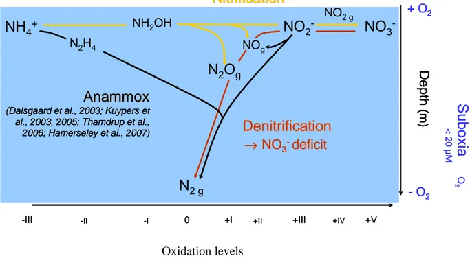
Oxygen Minimum Zones (OMZs) are oceanic areas which have concentrated much interest recently. They are characterized by low oxygen concentrations (even less than 1 mol L-1) and thus have a strong influence on biogeochemical cycles, greenhouse gases emission and life in the ocean. Denitrification is a common bacterial process occurring only in O2- deficient regions. Due to this process, nitrate is converted into radiatively active gaseous
nitrogen oxide which is released to the atmosphere (Cornejo and Farijas, 2012). This has a strong influence on nitrate to phosphate ratio which is lower than the canonical Redfield ratio of 16. Consequently, the phosphorus cycle is also influenced by the deoxygenation process. Lower ratios than Redfield of nitrate to phosphate have a strong impact on the carbon uptake by photosynthese processed and thus on the biological carbon pump.
Much of what we currently know about the temporal variability of biogeochemical processes comes primarily from in situ observations either ship-based, or from time series stations which give us just a limited understanding of how ocean biogeochemistry is changing in response to natural climate variations. The advent of satellite technology and the availability of satellite ocean colour allowed us to shed some more light on ocean biogeochemistry changes in response to El Niño for instance, or to anthropogenic climate changes driven by the accumulation of greenhouse gases in the atmosphere. The development of multi-disciplinary oceanic observatories for a long-time monitoring will help to increase the observing capacities in the constantly changing marine environment. This monitoring requires in situ miniaturized autonomous instrumentation able to achieve excellent figures of merit: long lifetime, high precision, low detection limit, fast response time, good reproducibility, resistance to biofouling and high pressure, able of stable long-term operation, and have low energy consumption. Within the past few years, sensor technologies for oxygen, chlorophyll, particles and nitrate have been refined (Johnson et al., 2009). These sensors are capable of deployment on long-endurance missions on autonomous platforms such as profiling floats and gliders.
For a large number of analytical methods, electrochemistry provides promising reagentless methods capable of miniaturization, have a decrease in response time with low energy requirements. In aquatic systems, electrochemical methods are used routinely for monitoring of pH by potentiometry, dissolved oxygen by amperometry (Revsbech et al., 2009), trace metals and speciation by voltammetry (Luther et al., 2001; Tercier-Waeber et al., 2005), conductivity and therefore salinity by impedimetry. Electrochemistry offers also a wide range of possibilities for achieving an excellent phosphate determination in seawater but
no autonomous electrochemical sensor for in situ phosphate determination currently existsts. Generally, the use of electrochemical in situ sensors in the ocean is not well developed but the opportunities provided by some teams show an increasing interest in this research field. My PhD thesis has two objectives:
A) Construction of an electrochemical sensor for in situ determination of phosphate in sea water,
B) Improvement of the STOX sensor for the determination of dissolved oxygen in the Oxygen Minimum Zones (OMZ).
The first part of the PhD thesis was performed in Toulouse, France in close cooperation with two laboratories: LEGOS (Laboratoire d’Etudes en Géophysique et Océanographie Spatiales) and LGC (Laboratoire de Génie Chimique).
The second part was carried out during a stage at Aarhus University and UNISENSE Company in Aarhus, Denmark.
This project is situated at the border of several fields: analytical chemistry, oceanography and biogeochemistry of the open ocean. Fundamentals of each of these disciplines must be presented here.
The first chapter is divided in two parts. The first part describes the biogeochemical cycles in the oceans related to the biological and physical carbon pumps. The phosphate chemistry and its special place in the biological carbon pump are also presented in this chapter. The second part is focused on the Oxygen Minimum Zone problem with a special attention on the influence of OMZs on the greenhouse gases budget and on biogeochemical cycles of nitrogen and phosphorus.
The second chapter is an overview of electrochemical techniques and is dedicated to non-specialists in this field. Firstly, principles of electrochemistry are described. Then electrochemical kinetics are presented with possible solutions of Fick’s diffusion law which is the basis of electroanalytical chemistry. Electrochemical techniques used in this work are recalled and finally the influence of adsorption and coupled chemical reactions on electrochemical signals is investigated.
The third chapter is a summary of the observing systems and autonomous in situ sensors deployed for phosphate and oxygen measurements in the ocean. It also includes the
various electroanalytical techniques used for phosphate detection in laboratory conditions. The crucial problem of corrosion and biofouling for deployments at sea is also addressed.
Chapter IV is a presentation of the work done during the secondment at Aarhus University. The work was focused on improvement of STOX sensor for detection of ultra-low oxygen concentrations by changing the method for front gold cathode formation. Firstly, the wet chemical method for gold plating on silicon membrane is described. Then a comparison of figures of merit for the traditional and improved STOX sensors is discussed.
Chapter V presents an additional work done on elucidation of complicated electrochemistry of isopoly- and heteropolyoxomolybdates formed during anodic oxidation of molybdenum in seawater. This work uncovers the chemical formulas of silico- and phosphomolybdate complexes and explains complicated electrode reactions. It thus helps to understand the difficulty of phosphate detection by electrochemistry.
Chapter VI is a presentation of the work done on development of phosphate sensor. The method is based on oxidation of molybdenum electrode in seawater in order to form phosphomolybdate complex, electrochemically detectable by means of amperometry or voltammetry. The construction of an electrochemical cell based on membrane technology done during this work gives the possibility to detect phosphate in presence of silicate without addition of any liquid reagents.
The final chapter is a description of work done on preliminary analysis of Peruvian water masses using data obtained during an oceanographic cruise offshore Peru. The CTD (Conductivity, Temperature, and Depth) data are supported by phosphate concentration profiles obtained by electrochemical measurements (as described in Chapter VI).
INTRODUCTION GENERALE (français)
L'eau a des propriétés « extraordinaires » qui jouent un rôle important dans le façonnement du climat sur Terre. La circulation océanique contribue à la répartition de la chaleur depuis les zones tropicales vers les pôles. De plus, les océans absorbent de grandes quantités de dioxyde de carbone de l'atmosphère. Environ un quart du dioxyde de carbone émis par les activités humaines se retrouve dans les océans (Balino et al., 2001; Denman et al., 2007), où il est en partie stocké et donc exclus de la circulation naturelle pendant plusieurs centaines d'années, contribuant ainsi à la réduction des effets du réchauffement climatique. Cependant, la nature ne reste pas indifférente à nos actions. L'élévation du niveau de la mer, les phénomènes météorologiques extrêmes, la désoxygénation et l'acidification des océans, la propagation des maladies tropicales, l'extinction d'espèces et les changements de structure et de fonctionnement des écosystèmes marins sont autant de conséquences des impacts des activités humaines sur le cycle naturel du carbone (Millero, 2007). Combien de dioxyde de carbone peut se dissoudre dans l'océan ? Quels sont les facteurs qui contrôlent ce processus et comment vont-ils changer dans le futur ? Une compréhension précise du cycle du carbone océanique permettra de répondre aux nombreuses questions posées par les scientifiques, les politiciens, les économistes, les industriels ... et permettra de les aider à comprendre, prédire, atténuer et même peut être « gérer » le changement climatique. Ceci ne représente pas une tâche facile parce que le cycle du carbone dans l'océan dépend de nombreux facteurs : la circulation océanique, les mécanismes biologiques de photosynthèse, de respiration et reminéralisation de la matière organique et les processus chimiques. La pompe biologique de carbone via le phytoplancton est contrôlée par la lumière et la disponibilité en macro- et micronutriments (phosphore, azote, silice et fer, etc.). Afin de mieux comprendre les
mécanismes inhérents à cette pompe, il convient d’établir une surveillance à long terme de cet environnement marin, environnement difficile d’accès car sombre et lointain, caractérisé par de fortes pressions, une grande variabilité de la température et de la salinité.
Les zones de minimum d'oxygène (OMZ) sont des régions océaniques où l’intérêt des oceanographes s’est concentré récemment. Elles sont caractérisées par des concentrations faibles en oxygène (moins de 1 mol L-1) et ont donc une forte influence sur les cycles biogéochimiques, les émissions de gaz à effet de serre et la vie dans l'océan. La dénitrification est un processus bactérien qui apparaît seulement dans les OMZ. En raison de ce processus, le nitrate est transformé en protoxyde d’azote, puissanr gaz à effet de serre qui est libéré dans l'atmosphère (Cornejo et Farijas, 2012). Le processus de désoxygénation a donc une forte influence sur le rapport N/P qui devient inférieur à la valeur canonique de 16 de Redfield. En conséquence, le cycle biogéochimique du phosphore est aussi influencé par la désoxygénation. Les rapports nitrate sur phosphate inférieurs à la valeur de Redfield ont un fort impact sur l’absorption du carbone par le processus de photosynthèse et donc sur la pompe biologique de carbone.
Une grande partie de ce que nous savons actuellement sur la variabilité temporelle des processus biogéochimiques provient principalement d’observations in situ, soit à partir de navires, soit à partir de stations de séries temporelles qui nous donnent cependant une compréhension limitée de la façon dont la biogéochimie des océans évolue en réponse aux variations naturelles du climat. L'avènement des missions satellitaires et de la disponibilité des données couleur de l’eau par satellite a permis une meilleure compréhension des changements biogéochimiques des océans en réponse au phénomène El Niño par exemple ou aux changements climatiques d’origine anthropique entraînés par l'accumulation de gaz à effet de serre dans l'atmosphère. Le développement des observatoires océaniques pour une surveillance continue de l’océan permettra d'accroître les capacités d'observation de l'environnement marin. Cette surveillance nécessite une instrumentation in situ miniaturisée, autonome, capable d'atteindre de hautes performances en terme de durée de vie, de précision de la mesure, de limite de détection, couplée avec un temps de réponse rapide, une faible consommation d’énergie, une bonne reproductibilité, une résistance aux biosalissures et aux hautes pressions. Ces dernières années, les technologies pour les capteurs d'oxygène, de nitrate, de chlorophylle, et du carbone particulaire ont été affinées (Johnson et al., 2009). Ces capteurs sont capables d’être délpoyé sur des missions longues sur des plateformes autonomes tels que les flotteurs profileurs et les planeurs.
Parmi le grand nombre de méthodes d'analyse, l'électrochimie permet d'aller plus loin dans la miniaturisation, de diminuer le temps de réponse et les besoins énergétiques, et donc dans le développement de méthodes prometteuses sans ajout de réactifs liquides. En milieu aquatique, les méthodes électrochimiques sont utilisées en routine pour la surveillance du pH par potentiométrie, l'oxygène dissous par ampérométrie (Revsbech et al., 2009), les métaux traces et leur spéciation par voltampérométrie (Luther et al., 2001 ; Tercier-Waeber et al., 2005), la conductivité et la salinité par impédance. L’électrochimie offre également un large éventail de possibilités pour parvenir à une excellente détermination du phosphate dans l’eau de mer, mais aucun capteur autonome pour la détermination électrochimique in situ des phosphates n’existe à ce jour. Globalement, l'utilisation de capteurs électrochimiques in situ dans l'océan n'est pas bien développée, cependant les possibilités offertes par certaines équipes montrent un intérêt croissant dans ce domaine de recherche.
Les travaux de ma thèse ont deux objectifs:
A) la construction d'un capteur électrochimique pour la détermination in situ de phosphate dans l'eau de mer,
B) l'amélioration de la sonde STOX pour la détermination de l'oxygène dissous dans les zones de minimum d'oxygène (OMZ).
La première partie de ma thèse a été réalisée à Toulouse, en France, en étroite coopération entre: le LEGOS (Laboratoire d’Etudes en Géophysique et Océanographie Spatiales) et le LGC (Laboratoire de Génie Chimique).
La deuxième partie a été réalisée au cours d'un stage de 3 mois à l'Université d'Aarhus et dans la compagnie Unisense à Aarhus au Danemark.
Ce projet de recherche est situé à la frontière de plusieurs champs disciplinaires : la chimie analytique, l'océanographie et la biogéochimie de l'océan ouvert. Les principes de base de chacune de ces disciplines seront présentés dans ce manuscript.
Le premier chapitre est divisé en deux parties. La première partie décrit les grands cycles biogéochimiques dans les océans en lien avec les pompes biologique et physique du carbone. La chimie des phosphates et sa place particulière dans la pompe biologique du carbone sont également présentées dans ce chapitre. La deuxième partie se concentre sur le problème des Zones de Minimum d'Oxygène avec une attention particulière sur l’influence des OMZs sur le budget des gaz à effet de serre et sur les cycles biogéochimiques.
Le deuxième chapitre est un aperçu des techniques électrochimiques et est plutôt dédié aux non-spécialistes dans ce domaine. Tout d'abord, les principes de l'électrochimie sont
décrits. Puis la cinétique électrochimique qui consitue la base de la chimie électroanalytique est présentée. Les techniques électrochimiques utilisées dans ce travail sont rappelées et nous discuterons enfin des problèmes d’adsorption et des réactions chimiques couplées.
Le troisième chapitre est un résumé des systèmes d'observation et des capteurs in situ autonomes déployés pour les mesures du phosphate et de l'oxygène dissous dans l'océan. Ce chapitre inclut une description des différentes méthodes d’analyse utilisées pour la détection de phosphates et d’oxygène dans des condtions de laboratoire, avec une attention particulière aux techniques électroanalytiques. Le problème crucial de corrosion et des biosalissures sera mentionné.
Le chapitre IV est une présentation du travail effectué pendant le stage à l'Université d'Aarhus. Ce travail a été axé sur l'amélioration du capteur STOX pour la détection d'oxygène à faible concentration. Cette amélioration a été effectuée par un changement dans la construction du capteur. Au lieu d'électrodéposer de l'or sur du platine, un dépôt d’or a été réalisé sur une membrane silicium afin de créer la cathode d’or. La comparaison entre le capteur STOX traditionnel et la version améliorée est discutée en fin de chapitre.
Le chapitre V présente un travail supplémentaire effectué sur l'électrochimie des complexes isopoly- et hétéropolyoxomolibdiques formés via l'oxydation du molybdène métal dans l'eau de mer. Ce travail a révélé la structure chimique des différents complexes silico- et phosphomolibdiques et a illustré la complexité des réactions électrochimiques et par conséquent la difficulté d’interprétation des signaux pour la détection des phosphates.
Le chapitre VI présente le travail effectué sur le développement du capteur de phosphate. Le procédé développé est basé sur l'oxydation d’une électrode de molybdène dans l'eau de mer pour former le complexe phosphomolibdique qui est ensuite détecté par ampérométrie ou voltammétrie. La réalisation d'une cellule électrochimique utilisant des membranes a permis de détecter les phosphates en présence de silicates sans addition de réactifs liquides.
Le dernier chapitre est une description du travail effectué sur l'analyse préliminaire des masses d’eaux péruviennes en utilisant les données obtenues au cours de la campagne océanographique au large du Pérou. Les données de CTD (Conductivité, Température, Profondeur) sont compilées avec les profils de concentration en phosphate obtenus par mesures électrochimiques (tel que décrits dans le chapitre VI).
CHAPTER I:
INTRODUCTION ON OCEAN BIOGEOCHEMISTRY AND ON
OXYGEN MINIMUM ZONES
The goals of this work were to develop an electrochemical sensor for phosphate detection in seawater and to improve an existing sensor for detection of ultra-low oxygen concentrations. A good understanding on ocean biogeochemical cycles in general and on the deoxygenation process is crucial for marine sensors development since it will help in finding solutions which respond to the needs of marine biogeochemists.
The basics of the ocean carbon cycle are firstly described. Both physical and biological pumps are discussed with a special attention to the factors controlling the biological CO2 uptake. Then the cycle of phosphate and its influence on the biological carbon
pump are discussed. The purpose of this part is to explain the importance of phosphate measurements in the general context of this project.
In the second section the deoxygenation issue associated to the Oxygen Minimum Zones is discussed and its impact on biogeochemical cycles and greenhouses emissions is mentioned. The biotic response to the Oxygen Minimum Zones is briefly presented. The purpose of this part is to explain the critical importance of oxygen ultra-low detection in the Oxygen Minimum Zones.
Contents:
1. Introduction on ocean biogeochemistry
21
1.1. The role of ocean in the global carbon cycle 21
1.1.1. The physical and biological carbon pumps 24
1.1.2. Human impact on ocean CO2 uptake 27
1.1.3. Oceanic circulation and global warming 28
1.2. The components of the biological carbon pump 29
1.2.1. Phytoplankton and primary production 29
1.2.2. Role of nutrients and iron in the biological carbon pump 32
1.3. The phosphate in the ocean 33
1.3.1. Chemistry of phosphate 33
1.3.2. The cycle of phosphate in the ocean 34
2. Introduction on Oxygen Minimum Zones (OMZs)
38
2.1. Oxygen in the ocean 38
2.2. Formation, distribution and stability of OMZ 40
2.3. The role of OMZ in the global climate change 42
2.3.1. Influence of OMZ on the biogeochemical cycles
and greenhouse gases budget 42
2.3.2. Biotic response to OMZ 43
1. Introduction on ocean biogeochemistry
Many closely related geological, physical, chemical, biological and biogeochemical processes take place in the ocean on a variety of spatio-temporal scales. The study of biogeochemical cycles of chemical elements (C, N, Si, P, Fe,...) requires taking into account the origins (sources), sinks and changes within each of the reservoirs (ocean, continent, atmosphere ...) of each element constituting them.
The carbon cycle in the global ocean includes the CO2 exchange at the
ocean-atmosphere interface, the general oceanic circulation, the riverine and eolian inputs of nutrients and inputs of nutrients by submarine volcanism. CO2 is one of the major greenhouse
gases with nitrous oxide and methane. The study of the carbon cycle is essential for understanding and predicting evolution of the climate. During photosynthesis, algae use energy from sunlight to convert CO2 and dissolved nutrients (nitrate, phosphate, silicate…) to
organic carbon. Monitoring levels of nutrients over time, as key elements of the marine food chain but also as tracers of water masses, is therefore a critical factor to ulimately monitor climate change.
1. 1. The role of the ocean in the global carbon cycle
The carbon cycle is the exchange of carbon among three reservoirs or storage places: land, oceans and the atmosphere (Figure I. 1.1). The atmosphere is the smallest pool of actively cycling carbon, that is, carbon which stays in a reservoir less than a thousand years or so. The land and its plants and animals, which are called the terrestrial biosphere, constitute the next largest reservoir of carbon and the oceans are the earth’s largest carbon active reservoir by far (Denman et al., 2007).
The processes by which carbon moves through the earth’s reservoirs take place on different time scales. The short-term carbon cycle includes processes that transfer carbon from one reservoir to another in a matter of years, including photosynthesis, plant and animal respiration, and the movement of CO2 across the air-sea interface. Other processes, such as
transformation of carbon into limestone and its subsequent release as the rock weathered, occur very slowly (thousands to millions of years). We call these processes the long-term carbon cycle.
Recent interest in the global carbon cycle corresponds to increasing levels of carbon containing gases like carbon dioxide (CO2), methane (CH4), carbon monoxide (CO), and
chlorofluorocarbons (CFCs). These gases are all radiatively active, that is, they trap the heat near the surface of the earth causing elevation of the average temperature. So, they are considered greenhouse gases (Millero, 2007).
Fig. I. 1.1. The global carbon cycle taken from the 4th IPCC Assessment Report, 2007. In the figure the carbon fluxes are shown in Gt C/yr with natural fluxes depicted by black arrows and the anthropogenic fluxes by red arrows (Denman et al., 2007).
The most important greenhouse gas is carbon dioxide (CO2). The amount of this gas is
increasing due to human activity. The pre-industrial level of this gas was 280 ppmV and has increased to the current levels of 370 ppmV (Figure I. 1.2). The levels of CO2 in the past
varied between 200 ppmV (glacial times) and 300 ppmV (interglacial times). More recent ice core measurements indicate that these levels have been similar for 600 ky (ky=1000 years) (Figure I. 1.3). These results indicate that the present level of CO2 in the atmosphere is 23%
higher than 280 ppmV in the past 600 ky (Siegenthaler et al., 2005). Thanks to its ability to buffer CO2, the oceans play a crucial role in regulation of the atmospheric level of this gas
interest in understanding the cycling of CO2 between the atmosphere and the oceans. The
influence of increasing CO2 levels on climate will be discussed later.
Fig. I. 1.2. The increase of carbon dioxide in the atmosphere at Hawaii from atmospheric sources and trapped in ice cores (Millero, 2007).
Fig. I. 1.3. The variations of carbon dioxide and temperature as recorded in the Vostok ice core during the last climate cycle (Millero, 2007).
Our present understanding of the temporal and spatial distribution of the net CO2 flux
into and out of the ocean is derived from a combination of field data, which is limited by sparse temporal and spatial coverage, and models, which are validated by comparisons with the observed distributions of tracers, like natural carbon-14 (14C), and anthropogenic chlorofluorocarbons, tritium (3H) and bomb 14C. With the additional data from global surveys of CO2 in the ocean (1991-1998), carried out during the Joint Global Ocean Flux Study
(JGOFS), the World Ocean Circulation Experiment (WOCE) Hydrographic Program, and during IMBER (Integrated Marine Biogeochemistry and Ecosystem Research) and SOLAS (Surface Ocean Lower Atmosphere Study) international cruises, it is now possible to characterize in a quantitative way the regional uptake and release of CO2 and its transport in
the ocean.
1.1.1. The physical and biological carbon pumps
The ocean plays an important part in both the organic and inorganic components of the carbon cycle. The ocean contains about fifty times more carbon than the atmosphere, but only 1 % of this carbon is in the form of CO2, most of the carbon is found as bicarbonate (HCO3-)
or carbonate (CO32-). CO2 dissolves in the ocean and reacts with water to form carbonic acid,
which rapidly dissociates into bicarbonate and carbonate ions according to the following equilibrium reactions (I. 1.1-1.3):
) ( ) ( 2 2 g CO aq CO (I. 1.1) 2 3 2(aq) H O H HCO CO (I. 1.2) 2 3 3 H CO HCO (I. 1.3)
The sum of CO2, HCO3- and CO32- is called Dissolved Inorganic Carbon (DIC); 91 %
of DIC is in the form of HCO3-, 8% in CO32- and only 1% in CO2 (Sarmiento and Gruber,
2001). Only CO2 is exchanged with the atmosphere due to physical and biological processes
known as physical and biological pumps presented in Figure I. 1.4.
The physical pump is driven by gas exchange at the air-sea interface and the physical processes that transport CO2 to the deep ocean. Atmospheric CO2 enters the ocean by gas
interface. The amount of CO2 absorbed by seawater is also a function of temperature through
its effect on solubility: solubility increases as temperature falls so that cold surface waters absorb more CO2 than warm waters. Generally speaking, cold and dense water masses in high
latitude oceans, particularly of the North Atlantic and Southern Oceans, absorb atmospheric CO2 before they sink to the ocean interior. The sinking is balanced by an upwelling in other
regions. Upwelled water warms when it reaches the surface where CO2 becomes less soluble
and some is released back to the atmosphere. The net effect is to pump CO2 into the ocean
interior (Maier-Reimer et al., 1996; Sarmiento and Gruber, 2002).
Fig. I. 1.4. The schematics of the biological and physical pumps (Chisholm, 2000).
Once CO2 is pumped to the ocean due to physical processes, the DIC is absorbed by
phytoplankton during photosynthesis. Using sunlight for energy and dissolved inorganic nutrients, phytoplankton convert DIC to organic carbon, which forms the base of the marine food web. When phytoplankton die or are eaten by zooplankton and higher trophic organisms, the part of the organic carbon from dead tissues can remain in the water as Dissolved Organic Carbon (DOC). The DOC can be transported by currents to deeper waters. Finally, another fraction of the organic carbon is transformed into aggregates called Particulate Organic Carbon (POC), which sink to greater depths. The carbon entrained in POC is remineralized by bacteria at depth and stored in the intermediate deep waters rich in carbon and transported back to the surface by ocean currents and vertical mixing (Chisholm, 2000). The food web's
structure and the relative abundance of species influence how much CO2 will be pumped to
the deep ocean. This structure is dictated also by the availability of inorganic nutrients such as nitrogen, phosphorus, silicon and iron. The influence of dissolved nutrients will be discussed in detail later.
Some marine organisms grow their shells out of calcium carbonate (CaCO3), changing
the surface water carbon chemistry. Shells sink in the deep water and the concentration of CO32- at the ocean surface decreases moving the equilibrium of reaction I. 1.4 towards the
right. ) ( 3 2 2 3 Ca CaCO s CO (I. 1.4)
Fig. I. 1.5. Annual exchange of CO2 across the sea surface (Takahashi et al., 2009).
Together with the solubility pump, the biological pump maintains a sharp gradient of CO2 between the atmosphere and the deep ocean. The annual CO2 exchange is presented in
Fig. I. 1.5. The blue and purple colours denote regions in which the ocean takes up large amounts of CO2, red and yellow colours mark regions in which large amounts of CO2 are
emitted into the atmosphere. The map shows that the Equatorial Pacific is the largest source of CO . This is due to the combination of strong upwelling of CO-rich waters and low
biological activity. The North Atlantic, on the other hand, is the most intense region of CO2
uptake in the global ocean. As the Gulf Stream and the North Atlantic Drift transport water northwards, it cools and absorbs CO2 from the atmosphere (Takahashi et al., 2009).
1.1.2. Human impact on ocean CO2 uptake
More than seven billion people burn fuel to keep warm, to provide electricity to light their homes, to run industry, and to use cars, buses, boats, trains, and airplanes. The burning of fuels adds about 6 gigatons of carbon to the atmosphere each year (Balino et al., 2001; Denman et al., 2007). The CO2 emitted into the atmosphere by human activities is taken up by
the ocean at a rate which depends primarily on the rate of increasing atmospheric CO2 as
compared with the rate of the ocean mixing. Nowadays, the ocean takes up about 2.2 PgC/yr (Denman et al., 2007, Gruber et al., 2009). However in the past 20 years models and observations suggest that the rate of growth of this sink may have slowed down (Canadell et al., 2007). Measurements show that the oceans have absorbed 29 % of the total CO2 emitted
since pre-industrial times (Sabine et al., 2004, Lee et al., 2003), but at present the ocean uptake is only 15% of the potential uptake level for an atmospheric concentration of 385 ppmV (Greenblatt and Sarmiento, 2004). Potential variations in the oceans’ sink efficiency due to climate change are extremely important because of the size of this sink. Several examples of influence of carbon dioxide increase on climate are discussed below.
The increase in the concentration of CO2 in the atmosphere will increase its flux across
the air-sea interface. This will result in a decrease in the pH of about 0.3-0.4 units if atmospheric CO2 concentrations reach 800 ppmv (Doney et al., 2009). The decrease in the pH
is expected to cause large changes in the carbonate system in the ocean. For example, organisms like pteropods, foraminifera, and cocolithophores will have difficulty with precipitating CaCO3; coastal corals may have difficulty in growing and may dissolve
(Beaufort et al., 2011). The constantly increasing carbon dioxide concentration in the atmosphere is causing the global increase of temperature. The carbon dioxide dissolves better in cold waters, thus increasing the temperature will cause the oceans to absorb less carbon dioxide than now, and this will result in strengthening the greenhouse gases effect. Moreover, higher temperatures will cause ice melting and greater inflows of freshwater into the oceans. In addition, higher temperatures, in accordance with the laws of physics, will lead to increased water volume. As an effect, this will lead to sea level rise and thus to intense flooding
(Millero, 2007). These are only a few examples of the effects of global warming. To understand, stop or mitigate these changes, we need to know first how the ocean machinery is functioning.
1.1.3. Oceanic circulation and global warming
The main forces driving oceanic circulation are the difference in density of different water masses and the winds. The density of seawater is controlled by its salinity and temperature. The salinity of the surface water is controlled mostly by the balance between evaporation and precipitation. As a result the highest salinities are found at low latitudes where evaporation is high and precipitation low. The temperature of the oceans depends mostly on the heat exchange with the atmosphere. In general the heat is transferred for low latitudes to high latitudes via the winds in the atmosphere and by the currents in the ocean (Wunsch, 2002; Colling, 2004). The thermohaline circulation known as the oceanic conveyor belt is a key regulator for climate (Figure I. 1.6). This circulation emphasises the interconnections among the waters of the world ocean.
Fig. I. 1.6. The thermohaline circulation of the oceans. Surface currents are shown in red, deep waters in light blue and bottom waters in dark blue. The main deep water formation sites are shown in orange (Rahmstorf, 2006).
Salty and warm surface waters reaching the high latitudes of the North Atlantic with the Gulf Stream are cooled in winter and sink to great depths and release heat. This heat helps to mitigate the climate in northern Europe. Deep waters being formed that way start their journey southwards where they join newly formed cold deep waters in Antarctica. Some then flow outward at the bottom of the ocean in the Atlantic, Indian and Pacific basins. These waters return to the North Atlantic as a surface flow, primarily through upwelling in the Pacific and Indian Oceans. The deep waters become enriched with essential nutrients and CO2
as they circulate, from organic matter decomposition in the water and sediments. A complete cycle of the conveyor belt takes about 1000 years.
There are evidences that the thermohaline circulation has changed regularly in the past (Rahmstorf, 2003, Toggweiler and Russell, 2008). The variation of climate due to changes in the circulation has been large, abrupt and global (Denton and Hendy, 1994; Clement and Peterson, 2008). One of the consequences of global warming will be an increase of sea surface temperature and the alteration of the hydrological cycle, both factors will make the formation of the salty deep water, which is the main driver of the ocean circulation, more difficult. Models used by the IPCC AR4 (Intergovernmental Panel on Climate Change, 4th Assessment Report: Climate Change 2007) show a reduction in the circulation by 15% to 50% in 2100 (Meehl et al., 2007).
1.2. The components of the biological carbon pump
If we wish to understand all the factors controlling the biological carbon pump in the ocean, both now and in the future as the ocean responds to global warming, then we must survey the oceanic biogeochemical cycles of phosphates, nitrate, iron and silicate. Generally, the access to carbon dioxide and sunlight is sufficient to start the photosynthesis process, but nutrients and iron concentrations are not similar in every region of the ocean and they play a main role in the biological carbon pump.
1.2.1. Phytoplankton and primary production
Phytoplankton are comprised of microscopic plants that live in the euphotic layer of the oceans. Most of them are simply drifting with the currents, but some may also move
independently. They use sunlight, micro- and macronutrients, carbon dioxide (CO2) in sea
water in a process called photosynthesis to produce organic matter, which they use as a building material for their own cells. In addition, during the photosynthesis process, phytoplankton release oxygen as a by-product (equation I. 1.5). Phytoplankton remove almost as much carbon dioxide from the atmosphere as terrestrial plants, and thus defines the Earth’s climate.
6 H2O + 6CO2 + h (energy) C6H12O6 + 6 O2 (I. 1.5)
Both the amount and the rate at which phytoplankton are produced are important to consider with respect to the availability of organic carbon in the food chain. The standing crop is the amount of living phytoplankton at a given time and a given amount of seawater (mg C m-3 of seawater) or at given surface of seawater (mg C m-2). The rate of primary
production (P) is defined as the weight of inorganic carbon fixed photosynthetically per unit
time per unit volume (mg C m-3 h-1) or under unit surface area (mg C m-2 day-1) (Millero, 2006). The new production is the primary production associated with newly available nitrogen (NO2-, NO3-, and NH). The new production plus the regenerated production (the
primary production associated with recycled nitrogen) are equal to the total primary production. These definitions are based on a system being in steady state. The ratio of the new production to the total production is called the “f” ratio. This ratio is useful in describing the
fraction of organic nitrogen and carbon exported from the surface waters to the deep ocean. It also represents the capacity of the system to sustain secondary and high levels of production.
A number of factors can affect the growth of phytoplankton in the ocean. One of the most important is light and thus, the sun’s altitude, cloud cover, and then reflection, absorption and scattering of light in water have a great influence on phytoplankton growth. The other important factor is salinity. Marine phytoplankton will grow at salinities as low as 15, some more successfully than at 35. Stenhaline organisms will only thrive in a limited range of salinity, for example Peridinium bacterium at salinity of 8-12 (Baltic Sea). Euryhaline organisms can live over a wide range of salinities. The temperature range in the ocean is -2° to 30°C. Phytoplankton are rapidly killed at temperatures 10° to 15°C above the temperature at which they are adapted to live. A slow decrease of the temperature has less of an effect (Millero, 2006).
Additionally, phytoplankton need nitrogen, phosphorus, iron and silicon for growth. This problem will be discussed later. Some organics are necessary as well: vitamin B and B
are growth promoters, ascorbic acid and cysteine may also be needed. The limitation in vitamin B12 inhibits the rates of photosynthesis by stopping cell division, causing a loss of
pigmentation and cell size (Millero, 2006).
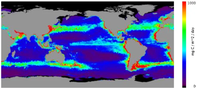
Regional differences make it a challenge to measure primary production of the ocean basins. Traditional techniques, based on discrete bottle samples, cannot give an accurate global picture. Recent advances in remote-sensing technologies have vastly improved estimates of primary production based on phytoplankton pigment levels. For instance, the Sea-viewing Wide Field-of-view Sensor (SeaWiFS), a satellite, mounted ocean colour instrument, measures chlorophyll (algal pigment) in every part of the global ocean. With these data now, it is possible to derive global seasonal to annual estimates of primary production (Fig. I. 1.7).
Fig. I. 1.7. Global ocean primary production estimated from chlorophyll a distribution derived from SeaWiFS data (www.science.oregonstate.edu/ocean.productivity).
The estimation shows very low primary production in the subtropical gyre regions of Pacific, Atlantic and Indian Ocean. These regions are called oligotrophic regions and are characterized by low nutrient concentrations. Eastern boundary regions (offshore Africa and Peru-Chile, for instance) are very productive due to upwelling phenomena which bring water masses rich in nutrients to the surface. Finally, there are the HNLC (High Nutrient Low Chlorophyll) zones characterized by high nutrient concentrations but low primary production due to limitation in iron and/or high rate of consumption of phytoplankton by zooplankton.
The HNLC regions are located in the Southern Ocean, in the equatorial band and in the subarctic Pacific Ocean.
1.2.2. Role of nutrients and iron in the biological pump
Phytoplankton need macronutrients, mainly nitrogen and phosphorus. Phytoplankton need nutrients in certain proportions according to the following reaction (Paytan and McLaughlin, 2007):
106 CO2 + 16 HNO3+ H3PO4 + 122 H2O + photons → (CH2O)106(NH3)16(H3PO4) + 138 O2
(I. 1.6)
For every 106 carbon atoms, which are processed in organic matter, it is necessary to use 16 nitrogen atoms and one phosphorus atom. These proportions are known as Redfield ratios (Redfield, 1958). Atmospheric nitrogen (N2) is usually not directly absorbed by
phytoplankton, although it can be by nitrogen fixers. Nitrate (NO3-) and ammonia (NH4+) are
the chemical substances being mostly uptaken by phytoplankton. In most areas of the ocean, nitrogen is lacking and we can say that the growth of phytoplankton is dependent on the availability of nitrogen. However, for example, in some oceanic areas, for instance in the eastern Mediterranean, it is the availability of phosphorus which determines the growth of phytoplankton. Natural sources of these nutrients are weathering of rocks (Paytan and McLaughlin, 2007) but also eolian and riverine inputs. Human activity also constitutes a source of nutrients. The main anthropogenic sources of phosphorus are detergents and sewage. The occurrence of nitrogen in waters is mainly due to intensive agricultural activities (Brandes et al., 2007) and coming from the excessive use of fertilizers containing nitrates and ammonia.
Another important nutrient is silicate, which is derived mainly from the weathering of rocks. The ratio of silicate over carbon varies from 0.06 and 0.45. Lack of silicate prevents the growth of certain species of phytoplankton, diatoms, which use this nutrient to build their skeletons. When running low on nitrogen or phosphorus, phytoplankton cease to grow. When running out of silicon, phytoplankton may continue growing, but a change in species composition may occur.
Phytoplankton also need a small amount of metal particles such as iron, copper, zinc and cobalt. The HNLC regions mentioned above do not have enough iron for phytoplankton to develop. These regions account for about 20% of the total area of the oceans. From the oceanographic point of view, these regions should be biologically active because they are located in upwelling regions. However, these regions are distant from the desert areas and very limited amounts of dust (and iron) reach the surface ocean (Sunda et al., 2010).
The so called iron limitation hypothesis has been tested by carring out in situ iron fertilization experiments for instance in the Southern Ocean (SOIREE, Jan ’99), similar to those carried out earlier in the eastern Pacific (IronEx I, 1993, and IronEx II, 1995). The
experiments showed enhanced phytoplankton growth and uptake of atmospheric CO2, but at
the same time a shift in the planktonic community was noticed (Balino et al., 2001; de Baar et al., 2005).
1.3. The phosphate in the ocean
As mentioned before, phosphate availability can impact primary production rates in the ocean as well as species distribution and ecosystem structure. Thus, the availability of phosphates in marine systems can strongly influence the marine carbon cycle and the sequestration of atmospheric carbon dioxide.
1.3.1. Chemistry of phosphate
From a chemical point of view, phosphates are the salts of phosphoric acid. In dilute aqueous solution, phosphate exists in four forms. In strongly-basic conditions, the orthophosphate ion (PO43-) predominates, whereas in weakly-basic conditions, the hydrogen
phosphate ion (HPO42-) is prevalent. In weakly-acid conditions, the dihydrogen phosphate ion
(H2PO4-) is the most common. In strongly-acid conditions, aqueous phosphoric acid (H3PO4)
is the main form. More precisely, considering the following three equilibrium reactions:
2 4 4 2PO H H PO H (I. 1.7) 2 4 4 2PO H HPO H (I. 1.8)
3 4 2 4 H PO HPO (I. 1.9)
the corresponding constants at 25°C (in mol/L) are:
7.5 10 3, 1 2.12 4 3 4 2 1 a a pK PO H PO H H K (I. 1.10)
6.2 10 8, 2 7.21 4 2 2 4 2 pK PO H HPO H Ka (I. 1.11)
2.14 10 , 3 12.67 13 2 4 3 4 3 a a pK HPO PO H K (I. 1.12)1.3.2. The cycle of phosphate in the ocean
The phosphorus content on both oceans and land is very small. The main reservoir of phosphorus on land is rocks formed in ancient geological epochs. These rocks gradually ventilate and release phosphorus compounds into marine ecosystems. Continental weathering is the primary source of phosphorus to the oceanic phosphorus cycle. Most of this phosphorus is delivered via rivers with a smaller portion delivered via dust deposition. In recent times, anthropogenic sources of phosphorus have become a large fraction of the phosphorus delivered to the marine environment, effectively doubling the pre-antrophogenic flux. The main anthropogenic sources of phosphorus are detergents and sewage. The primary sink for phosphorus in the marine environment is the loss to sediments. Much of the particulate flux from rivers is lost to sediments on the continental shelves, and a smaller portion is lost to deep-sea sediments. In surface waters, certain phosphate forms (PO43-) are taken up by
phytoplankton during photosynthesis. Subsequently, the phosphate travels up through the food chain to zooplankton, fish and other top marine organisms. Much of organic-P is converted back to PO43- in surface waters as phytoplankton die but some of it finds its way to
the deep ocean (via downwelling and sinking of organic matter) where it is remineralized back to inorganic-P. It may return to the surface waters (via upwelling) or be bound by the widely prevalent cations (Al3+, Ca2+, Fe2+, Fe3+) and stored as minerals for a long time in the rocks and sediments. In that case, only geological processes can bring them back to cycle. The processes described above are presented in Fig. I. 1.8 as the marine phosphorus cycle with a special attention to different phosphorus fluxes.
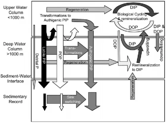
The transformations between the various phosphate (DIP, DOP, PIP, POP) forms in the water column and sediments, shown in Fig. I. 1.9, allow a better understanding of the oceanic phosphate cycle.
Fig. I. 1.9. Transformation between phosphorus forms in the water column and sediments. (Paytan and McLaughlin, 2007) (DIP-dissolved inorganic phosphorus, DOP-dissolved organic phosphorus, PIP-particulate inorganic phosphorus, POP-particulate organic phosphorus).
Vertical sections for phosphate concentrations in sea water are presented in Fig. I. 1.10 for the Atlantic, Pacific and Indian Oceans. As phytoplankton and other organisms die, PO4
3-is regenerated in the water column. A maximum regeneration occurs near 1000 m, which 3-is the same depth as the oxygen minimum layer. The maximum values of phosphate concentration in the Atlantic are about 2.5 M, while in the Pacific values around 3.25 M occur. The higher values observed in the Pacific (and Indian) oceans as compared to the Atlantic are due to the age of the water masses (older in the Pacific thus accumulating more oxidized plant material). Generally, knowledge of the phosphate concentration in the ocean surface allows us to deduce information on the biological activity in the ocean. Secondly, phosphate is one of the chemical tracers (along with temperature, salinity, other nutrients concentration…) which allows us to analyse water mass mixing and determine the origin of the water masses.
Fig.I. 1.10. Vertical section of phosphate concentrations obtained during the campaign WOCE A16, P16 and Indian Ocean 18.
2. Introduction on the Oxygen Minimum Zones (OMZs)
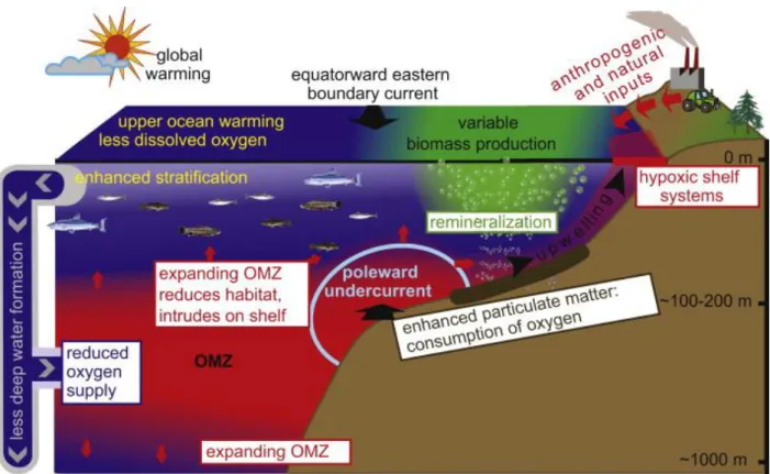
For various reasons, the content of the global ocean dissolved oxygen is far from uniform. In some places, hypoxia (oxygen deficiency) occurs and strongly affects the biological activity in the first few hundred meters depth. These regions are called the Oxygen Minimum Zones (OMZ) and are found in tropical regions, in the eastern Pacific and northern Indian Ocean. They are usually associated with upwelling systems and their extent increases in summer and reduces in winter. Global warming is expected to help expand the OMZ and to increase the hypoxia (Oschlies et al., 2008; Stramma et al., 2008; Keeling et al., 2010). Models indicate that the average concentration of oxygen should decrease as well (Stramma et al., 2012). These regions are still rather poorly understood despite much recent interest. A better understanding of biological, biogeochemical and physical processes in these regions will help us to answer many questions about the OMZ’s formation and expansion, and its influence on ocean’s life, biogeochemical cycles of phosphorus, nitrogen and carbon and emission of greenhouse gases to the atmosphere.
2.1. Oxygen in the ocean
The most studied gas (other than CO2) is dissolved oxygen. The oxygen cycle is very
complicated due to the fact that it participates in the composition of many compounds. Sources of oxygen in natural waters are the process of absorption of oxygen from the atmosphere, the formation of oxygen as a result of the photosynthesis and the entering oxygen from rain and snow water. The distribution of oxygen in the oceans is the net result of (Millero, 2006):
- Near equilibrium of atmospheric oxygen in the surface mixed layer - Biological production in subsurface waters caused by photosynthesis
- Biological use of oxygen in respiration in all waters and oxidation of plant material in intermediate waters
- Increases in oxygen in deep waters caused by the sinking of cold water rich in oxygen.
Fig.I. 2.1. Vertical section of oxygen concentrations obtained during the campaigns WOCE A16, P16 and Indian Ocean 18.
The dissolved oxygen concentrations decrease with depth in the ocean (to reach minimum values at depth of about 1000 m) due to utilization of oxygen for oxidation of organic substances and respiration of aquatic organisms. At greater depths the concentrations of oxygen increase slightly again as presented in Figure I. 2.1. Normally, the concentration of oxygen is sufficient for sustaining life of marine organisms. However, in Oxygen Minimum Zones a severe reduction or in extreme cases the complete loss of animal life may occur.
2.2. Formation, distribution and stability of the OMZ
Oxygen Minimum Zones are the regions in aquatic systems where concentrations of oxygen are as low as a few M. Oxygen Minimum Zones constitute primarily a problem in Eastern Boundary Upwelling Systems (EBUS), some coastal waters and enclosed seas (Fig. I. 2.2), although it can also be an issue in freshwater lakes. Vertical oxygen profiles in the OMZs are different from the classical O2 minimum profiles (Fig. I. 2.2). The oxygen
minimum is 5 times shallower up to 100-200 m than in the oxygenated ocean including a marked gradient, the oxycline (Paulmier and Ruiz-Pino, 2009) and it is also 50 times more intense. The total area of permanent OMZs is 8% of the global oceanic area and these include mainly: the Eastern South Pacific, Eastern Tropical North Pacific, the Black Sea, the Arabian Sea and Bay of Bengal. Oxygen Minimum Zones result from the combination of complex ecological phenomena that arise from the convergence of several factors:
- Physical environment: In these oceanic areas, ventilation is very weak due to a sluggish
circulation and in EBUS undercurrents usually advect low oxygen waters. Wind strength and direction also affect the rate of mixing. Poorly-mixed waters increase the chance that an OMZ might develop.
- Nutrient enrichment: An overabundance of nutrients, combined with enough light and
warm, slow-moving, and poorly-mixed water, can result in algae blooms and eutrophication. This is a prerequisite for the chain of reactions leading to OMZ formation. These overabundant nutrients may come from both natural sources (upwelling) and human activities.