Developments in finite element simulations of continuous casting

Main title: Developments in finite element simulations of continuous casting. Author names: S. Castagne, F. Pascon, G. Blès and A.M. Habraken.

Addresses: Institute of Mechanics & Civil Engineering University of Liège

M&S Department

Chemin des Chevreuils, 1 B-4000 Liège 1

Belgium

S. Castagne, F. Pascon, G. Blès and A.M. Habraken

Abstract. Two complementary approaches of steel continuous casting modelling using the finite element code

LAGAMINE have been developed in the M&S Department. We propose here a description of the context in which the study started, then a description of both macroscopic and mesoscopic approaches. The first one describes the whole continuous casting process, from the free surface in the mould and through the entire machine, including thermal and mechanical behaviour of the steel. The second approach focuses on the prediction of cracks and is developed at the grain scale. Some results are also presented for both models.

1. CONTEXT OF THE STUDY

Transverse cracking is recognized as a problem in continuous casting of low carbon steel. Experimental studies have demonstrated that such steel grade is more brittle in the temperature range from 1000 to 600 °C [1]. During the bending and unbending operations of the strand, this loss of ductility results in initiation of cracks, which have been shown to be intergranular. The measures to prevent transverse cracking are divided into two parts: certainly the control of the steel chemistry but also the prevention of the crack initiation and propagation due to thermomechanical loadings during the process. This second point is the principal objective of our study.

Two complementary models are proposed. The macroscopic one provides various results such as temperature field, thickness of the solidified shell, stress, strain and strain rate fields in the strand. The strain and stress history can be used to predict damage thanks to the accumulative values of macroscopic fracture criteria implemented in the code. This is an uncoupled approach where the damage is computed from the stress and strain fields but has no influence on them. On the other hand, the mesoscopic model aims at studying crack initiation and propagation in the process and especially during the unbending operation of the strand. This is a coupled approach: the damage processes are incorporated into the constitutive relations and the redistribution of stresses due to crack propagation is taken into account. The damage model uses a numerical mesoscopic approach identified by experimental measurements obtained at the microscopic and macroscopic scales. The mathematical model development begins with the construction of a 2D representative mesoscopic cell which is loaded by stress and strain fields determined by macroscopic experiments. Such an approach allows the identification of the damage law. Concerning the application to continuous casting, the macroscopic model gives the loading (stress, strain and temperature fields) to apply to the mesoscopic cell.

2. MACROSCOPIC APPROACH OF THERMO-MECHANICAL BEHAVIOUR

2.1 Global approach

A thermo-mechanical macroscopic model has been worked out using a non-linear finite element code, called LAGAMINE, which has been developed since early eighties at University of Liege for large strains/displacements problems, more particularly for metal forming modelling. Since a complete 3D

discretization of continuous casting seemed impossible to manage (both because of numerical stability and convergence reasons, but also computing time), a 2D½ model has been preferred.

This model belongs to the “slice models” family. We can summarise the approach as follows: we model with a 2D mesh a set of material points representing a slice of the steel strand, perpendicularly to the casting direction. Initially the slice is at the meniscus level and its temperature is assumed to be uniform and equal to the casting temperature. Since this slice is moving down through the machine, we study heat transfer, stress and strain development and solidification growth, according to boundary conditions. 2.2 Mechanical model

2.2.1 Generalized plane strain state

From a mechanical point of view, the slice is in generalised plane strain state (2D½). That means that the thickness t of the slice is governed by the following equation:

0 1 2

( , )

t x y =α +α x+α y (1)

where α0, α1, α2 are degrees of freedom corresponding respectively to the thickness at the origin of the axes (α0) and the variation of thickness along axes x (α1) and y (α2), both directions in the plane of the slice.

This formulation allows at the same time stresses and strains in the out-of-plane direction, which means in the casting direction. It is thus more complete than classical 2D approaches (plane strain/stress state) and much less CPU expensive than 3D approach.

Moreover, it allows the modelling of bending and straightening of the strand, enforcing a relation between αi degrees of freedom so that the correct radius of curvature of the machine is respected.

Last but not least, this 2D½ also permits to apply a force in the casting direction, which is of prime importance since it was necessary to take into account the withstanding force of the strand due to friction in different places in the machine.

2.2.2 Constitutive law

The mechanical behaviour of steel is modelled by an elastic-viscous-plastic law. The elastic part is governed by a very classical Hooke's law. In the viscous-plastic domain, we developed a Norton-Hoff type constitutive law [2], the expression of which (in terms of Von Mises equivalent values) is:

1 3 4

2

3.p e. pε.( 3. ) .p p

σ ₌ − ε_& ε

(2) where p1,2,3,4 are temperature dependent parameters, which can be fitted on experimental curves.

According to the assumptions of Von Mises loading surface, associated plasticity and normality in Prandtl-Reuss flow law, the expression (2) becomes in terms of deviatoric tensors:

(

)

= and the integration of this constitutive law is based on an implicit scheme. All the parameters are thermally affected.

2.2.3 Ferrostatic pressure

The liquid pool in the middle of the strand applies a hydrostatic pressure on the solidified shell. This pressure is called ferrostatic pressure pf and it is equal to:

(

)

f s

where γ is the volumetric weight of steel, D the depth under the meniscus level and fs the solid fraction. Since the studied steel is not an eutectic composition, solidification occurs over a range of temperature limited by the solidus temperature (Tsol) and the liquidus one (Tliq). We assume a linear variation of the solid fraction according to temperature in this range:

( )

0 _s liq 1 _liq, _sol

liq sol T T f T T T T T T − ⎡ ⎤ ≤ = ≤ _{∀ ∈ ⎣ ⎦} − (5)

Since the liquid pool applies the ferrostatic pressure on the solidified shell, the strand bulges between the rolls. The maximum bulging must be controlled, otherwise the slice model gives a wrong value because of the lack of continuity in the casting direction. Some springs, the stiffness of which being fitted, allow to insert in the model a force corresponding to the shear stress in the casting direction. This way, the bulging has been controlled using the prediction of the maximum bulging based on a model taking into account the casting speed, the steel grade, the geometry and temperature.

2.3 Thermal aspects

2.3.1 Internal heat conduction

The heat transfer in the material is govern by the classical Fourier's law, expressing the energy conservation and taking into account the release of energy during phase transformation (solidification is exothermic):

(

)

where H is the enthalpy, T the temperature and λ the thermal conductivity of the material. The enthalpy H is given by:

(

)

H =

∫

where ρ is the volumetric mass, c the specific heat and LF the latent heat of fusion.

2.3.2 Thermal shrinkage

Thermal shrinkage εthermdue to solidification is given by:

( )

therm _{T T I}

ε_& =α ⋅ ⋅& (8)

where I is identity tensor and α is the linear thermal expansion coefficient, which is thermally affected.

2.4 Boundary conditions

Different boundary conditions can occur, according to the position of the slice in the machine and the contact conditions. Table 1 summarizes the different cases.

In case of mechanical contact, the normal pressure is calculated by allowing, but penalizing, the penetration of bodies into each other. The friction τc is then computed with the Coulomb's friction law:

.

c µ n

τ = σ (9)

The heat transfer q from the strand to the ambient is given by the simple relation:

(

)

q=h T −T (10)

where h is the heat transfer coefficient according to the boundary conditions (Tab. 1). In case of contact, h is the inverse of the contact thermal resistance. In case of water spray cooling, h has been experimentally determined for different temperatures (700-1200 °C), different shapes of spray, different rates of flow and at different distances from the nozzle.

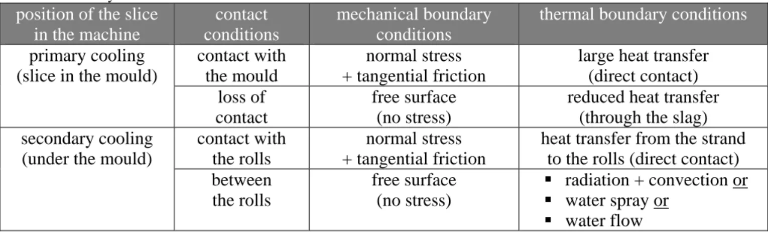
Table 1. Boundary conditions

position of the slice in the machine

contact conditions

mechanical boundary conditions

thermal boundary conditions

primary cooling (slice in the mould)

contact with the mould

normal stress + tangential friction

large heat transfer (direct contact) loss of

contact

free surface (no stress)

reduced heat transfer (through the slag) secondary cooling

(under the mould)

contact with the rolls

normal stress + tangential friction

heat transfer from the strand to the rolls (direct contact) between the rolls free surface (no stress) ƒ radiation + convection or ƒ water spray or ƒ water flow 2.5 Industrial applications

A first industrial application was the study of the influence of the mould taper on the cooling rate during the primary cooling [3]. The bases of the model had already been developed and some interesting results led to use now the model in order to evaluate the efficiency of a given taper for the casting of relatively complex cross sections (such as beam blanks, the optimal mould taper of which is not easily determined as for simple cross section such as round or squared billets).

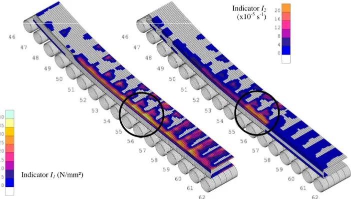
In the last three years, another industrial application has been performed. This time, the purpose of the study was to evaluate the influence of some local defects (such as nozzle perturbation, roll locking or roll misalignment) on the risk of transverse crack initiation. The first way to do so was to define some “macroscopic” indicators of crack initiation. We used the two following ones, both combining the gap of ductility of steel in a given range of temperature (TA-TB for a given steel composition) and the

mechanical loadings in the direction of casting: the longitudinal stress for the first indicator I1 and the longitudinal strain rate for the second one I2.

(

)

[

]

[

]

(

)

[

]

[

]

As it clearly appears, these indicators are different of zero only if the temperature corresponds to the range of temperature in which the ductility of the material is low and if the loading is in the sense of opening a crack (tensile stress or elongation). In such a case, the higher the loading is the higher the value of the indicators are. In any other case, the indicators are equal to zero, meaning that the risk of transverse crack initiation vanishes.

The model provides many results; among others temperature evolution (thus surface temperature, evolution of solidification, metallurgical length…), stress and strain states (and combinations such as indicators defined here above), bulging between rolls, extracting force.

Figure 1 represents a part (straightening zone) of the casting of a microalloyed steel with standard conditions (without any local defect). The figure shows the value of the 2 indicators and the localization of the maximum values (maximum risk) accords with observation.

Other computations including local defects have been performed. Comparing the following reference case (standard conditions) to the value of the indicators in each defect case, we studied the effect of each defect. This comparison allowed us to classify the defects from the less to the most critical.

Indicator I2

(x10-5 s-1)

Indicator I1 (N/mm²)

Figure 1. Indicators of risk of transverse crack initiation with standard casting conditions (reconstituted 3D view of the

surface of the cast product – ½ structure because of symmetry).

3. MESOSOPIC MODEL

3.1 Mesoscopic cell

The austenitic grain boundary is a favourable place for cracks to begin. They appear by strain concentration and microvoid coalescence at grain boundaries and by grain boundary sliding [4]. The influence of creep, controlled by diffusion, is important in the studied temperature range (between 800°C and 1000°C during the unbending phase).

In order to represent intergranular creep fracture, the developed model contains solid finite elements for the grains and interface elements for their boundaries (see also [5]). Inside the grains, an elasto-visco-plastic law without damage is used, and at its boundaries, a law with damage is preferred.

The mesoscopic approach allows a parametrical study of various factors such as grain size, precipitation state or oscillation marks geometry. The model can be applied to the continuous casting process as we know the loading to apply in the critical zone thanks to the macroscopic approach. As we want to analyse the process at the grain scale, we have to concentrate on specific zones.

3.1.1 Solid finite elements and grain representation

Grains are modelled by thermomechanical 4-nodes quadrilateral solid elements BLZ2T of mixed type [6]. Metallographic and texture analysis combining optical microscopy, scanning electron microscopy and orientation image microscopy, as well as various chemical etching and visual observation on steel samples, have been performed at room temperature to determine the previous austenitic grain size and morphology. Hence the geometry of the mesoscopic cell is defined taking into account the results of this micrographic study.

The Norton-Hoff law (2) is used to quantify the visco-plastic behaviour inside the grain for the studied steel. Compression tests of cylindrical samples have been performed after a thermal treatment aiming to reproduce the thermal cycle in continuous casting. Various strain rates and temperatures have been tested and compared with simulations in order to identify the parameters of this mechanical law.

3.1.2 Interface finite elements and grain boundary representation

The relevant damage mechanisms at the mesoscale are viscous grain boundary sliding, nucleation, growth and coalescence of cavities leading to microcracks. The linking-up process subsequently leads to the formation of a macroscopic crack.

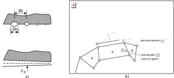
The solid elements that model the grains are connected by interface elements to account for cavitation and sliding at the grain boundary. As the thickness of the grain boundary is small in comparison with the grain size, the grain boundary is represented by one-dimensional interface elements. These elements are associated with a constitutive law which includes parameters linked to the presence of precipitates, voids, etc. The damage variable explicitly appears in this law.

2a 2b

δ c

a) b)

Figure 2. a) Discrete and continuous representations of the grain boundary. b) Interface element: contact element, associated

foundation, linked solid elements. Dots symbolize nodes and crosses represent integration points.

The interface element is composed of a modified contact element and a foundation element (Fig. 2b). For each integration point of the contact element, the program determines the associated foundation segment as well as the solid element to which the foundation is associated. The state variables for the interface element are computed using pieces of information of the two solids elements in contact (elements i and j in Fig. 2b). The state variables in the interface element are the corresponding mean values at the integration points of elements i and j.

The original contact element is described in [7] and is usually combined with the Coulomb’s friction law (9). This element has been modified in order to introduce a new interface law and a cohesion criterion. The stress components of the interface element are represented by Figure 2, their evolution is described by the following viscoelastic-type relationships:

(

)

(

)

= − = & &−

& k u us & &s &n kn c

τ σ δ δ

)

(13) This is a penalty method where penalty coefficient ks and kn, are very large to keep the deviations

(

(

)

to shear stress τ and the average separation rate, normal to the interface and the foundation, due to damage growth. These variables are directly computed from nodal displacements. The evolution of u &s

and of &δ_c are computed hereafter (equations (14) and (15)). More details can be found in [8]. Grain boundary sliding is governed by:

s B u w τ η = & (14)

where u_&s is the relative velocity between two adjacent grains, w is the thickness of the grain boundary and ηB is the grain boundary viscosity.

The discrete cavity distribution is replaced by a continuous distribution on each facet of the grain boundary so that the cavity volume V and the average separation between two grains δC evolve in a

continuous way on the facet (Fig. 2a). Then, the separation rate is given by:

2 2 2 c V V b b δ π π = & − & & b b (15)

In this equation, the cavity volume growth rate V depends on several variables and parameters such as strain rate, stresses at the grain boundary, diffusion in the material and creep exponent. The evolution rate of the cavity spacing b is linked to the nucleation activity.

&

&

The coalescence takes place when cavities are sufficiently close to each other to collapse. At this moment, the crack begins to propagate and the interface elements are no more in contact. For Onck [5], the parameter used to define the coalescence activation is the ratio a/b with a and b defined on Figure 2a.. We call it a damage variable in our model. When this ratio reaches the value 0.7, coalescence is triggered and crack appears.

3.2 Meso-macro link

3.2.1 Description of the method

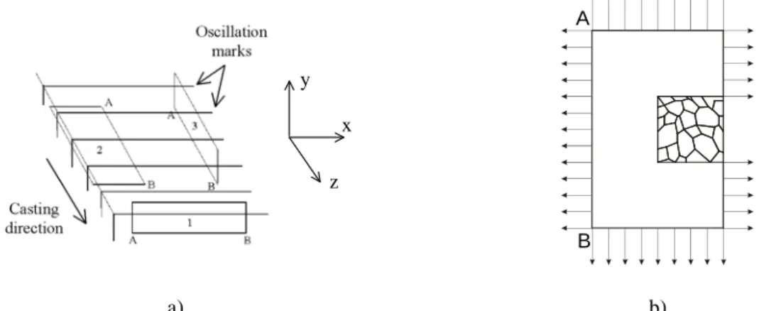
Transverse cracks always appear near the edge of the slab and at its surface. The mesoscopic cell is chosen in this zone, perpendicular to the oscillation marks if we want to study their influence (sections 2 and 3 on Fig. 3a).

The mesoscopic cell is surrounded by a transition zone which allows the transfer of data from the macroscopic model. It is important to follow the whole process as we use elasto-visco-plastic constitutive laws. The history of displacements known thanks to the macroscopic simulation is imposed on each node of the boundary of the transition zone as shown on Figure 3b. With these boundary conditions, the crack is free to initiate in the mesosopic cell.

z x y A B a) b)

Figure 3. a) Piece of slab: position of the studied sections. b) Mesoscopic cell surrounded by the transition zone, arrows

indicate imposed displacements, oscillation marks can be introduced on the right border for sections 2 and 3.

At each time step, the temperature of each node is fixed according to the results of the macroscopic simulation and no thermal exchange is computed at this scale. Indeed, all the thermal problem has already been treated in the macroscopic model.

3.2.2 Results

Growth of cracks for the simple loading of Figure 4a is simulated as a first application. The parameters for the interface law are issued from [5]. The displacement rate is chosen to obtain strain rates compatible with those usually encountered in continuous casting. Application of actual loadings issued from the

macroscopic model has still to be done. Nevertheless, with this first example, the stability of the code when a crack is propagating can be analysed.

The mesh is defined on the basis of a micrograph realised on a low carbon steel. A special etching was previously done to locate the austenitic grain boundaries. The size of the mesoscopic cell is 5x5 [mm] and it is surrounded by a transition zone (10x15 [mm]). We remark that the austenitic grain size is quite large. < -42 -21 0 21 42 64 85 106 128 149 171 192 > 213 a) b) c) d) e)

Figure 4. a) Imposed displacements. b-e) Stress maps σm [MPa] at different steps of the crack propagation.

On Figure 4b-e, we detect two cracks initiating and propagating along grain boundaries. Stresses concentrate around the crack tip and decrease on the border of the crack.

4. CONCLUSIONS

Two models analysing the continuous casting process have been proposed. The macroscopic one provides results such as temperature evolution, stress and strain states for the whole process and indicators for the critical zone. Various practical defects can be compared.

The development of the mesoscopic model is still progressing. The first application with a mesh representing real grains has shown that it is possible to follow initiation and propagation of crack with this approach. Industrial practical cases have now to be tested.

Acknowledgement

As Research Associate of National Fund for Scientific Research (Belgium), A.M. Habraken thanks this Belgian research fund for its support. Industrial partner ARCELOR and its research teams IRSID and the Technical Direction of Cockerill Sambre are also acknowledged.

References

[1] H. Suzuki, S. Nishimura, J. Imamura and Y., Transaction ISIJ, Vol. 24 (1984), 169-177.

[2] Habraken A.M., Charles J.F., Wegria J. and Cescotto S., Int. J. Forming Processes Vol. 1, n°1 (1998), 53-73.

[3] Pascon F., Habraken A.M., Bourdouxhe M. and Labory F., Mec. Ind., Vol. 1 (2000), 61-70. [4] B. Mintz, S. Yue and J.J. Jonas, International Material Reviews, Vol. 36, n°5 (1991), 187-217. [5] P. Onck and E. van der Giessen, J. Mech. Phys. Solids, Vol. 47 (1999), 99-139.

[6] Y. Zhu and S. Cescotto, Int. J. Num. Meth. Eng., Vol. 38, (1985) 685-716.

[7] A.M. Habraken and S. Cescotto, Mathl. Comput. Modelling, Vol. 28 (1998), 153-169.

[8] S. Castagne, M. Remy and A.M. Habraken, Proc. 6th Asia Pacific Symposium on Plasticity and Its Application, Sydney (2002), 145-150.