Science Arts & Métiers (SAM)
is an open access repository that collects the work of Arts et Métiers Institute of Technology researchers and makes it freely available over the web where possible.
This is an author-deposited version published in: https://sam.ensam.eu
Handle ID: .http://hdl.handle.net/10985/9867
To cite this version :
José OUTEIRO, Domenico UMBRELLO, Rachid M'SAOUBI, I.S. JAWAHIR - Evaluation of present numerical models for predicting metal cutting performance ans residual stresses -Machining Science and Technology - Vol. 19, p.183-216 - 2015
Any correspondence concerning this service should be sent to the repository Administrator : [email protected]
EVALUATION OF PRESENT NUMERICAL MODELS FOR PREDICTING METAL CUTTING PERFORMANCE AND RESIDUAL STRESSES
Jos ´e Carlos Outeiro1, Domenico Umbrello2, Rachid M’Saoubi3, and I. S. Jawahir4
1LaBoMaP, Arts et M´etiers ParisTech, Cluny, France
2Department of Mechanical Engineering, Energy and Management Engineering, University of Calabria, Rende, Italy
3R&D Materials and Technology Development, Seco Tools AB, Fagersta, Sweden 4Institute for Sustainable Manufacturing (ISM), University of Kentucky, Lexington, Kentucky, USA
✷ Efforts on numerical modeling and simulation of metal cutting operations continue to increase
due to the growing need for predicting the machining performance. A significant number of numer-ical methods, especially the Finite Element (FE) and the Mesh-free methods, are being developed and used to simulate the machining operations. However, the effectiveness of the numerical models to predict the machining performance depends on how accurately these models can represent the actual metal cutting process in terms of the input conditions and the quality and accuracy of the input data used in such models. This article presents results from a recently conducted comprehensive benchmark study, which involved the evaluation of various numerical predictive models for metal cutting. This study had a major objective to evaluate the effectiveness of the current numerical predictive models for machining performance. Five representative work materials were carefully selected for this study from a range of most commonly used work materials, along with a wide range of cutting conditions usually found in the published literature. The differences between the predicted results obtained from the various numerical models using different FE and Mesh-free codes are evaluated and compared with those obtained experimentally.
Keywords benchmark, machining, numerical simulation, surface integrity
INTRODUCTION AND METHODOLOGY
Modeling and simulation of metal cutting operations have become very popular in recent times with many universities, research institutions and companies developing and/or using various models to predict the ma-chining performance in terms of cutting forces, temperatures, hardness,
Address correspondence to J. C. Outeiro, Arts et M´etiers ParisTech, Centre of Cluny, Rue Porte de Paris, F-71250 Cluny, France. E-mail: [email protected]
Color versions of one or more of the figures in the article can be found online at www.tandfonline.com/lmst.
microstructural and phase changes, residual stresses, tool-wear, part dis-tortion, surface roughness, chip breaking/breakability, process dynamics, stability of machining operations, etc. (Altintas and Budak, 1995; Arrazola et al., 2013; Mabrouki et al., 2008; Outeiro et al., 2006b; Umbrello et al., 2007, 2010; Valiorgue et al., 2007). However, the effectiveness of these mod-els to predict the machining performance has been questionable due to poor representation of the actual metal cutting process in these models in terms of the assumptions made and the boundary conditions used in these models, including the quality and accuracy of the input data used in such models.
Over the last few decades, analytical and empirical models were most commonly developed and applied to predict mainly cutting forces and tem-peratures. However, since the early 1980s, the rapidly increased computa-tional capabilities, with the use of computer-based modeling and simulation methods based on Finite Element Method (FEM), have gained a signifi-cant application potential. Today, these models have a prominent place in the metal cutting simulation, although it must be stated very clearly that the FEM-based models inherently incorporates many simplistic assumptions that cannot be easily detected by its users, but that affect the validity of the results (Astakhov and Outeiro, 2008).
Within the scope of the recent CIRP (The International Academy for Production Engineering) Collaborative Working Group (CWG) on Sur-face Integrity and Functional Performance of Components, which oper-ated during 2007–2011, it was decided to conduct a benchmark study to evaluate the effectiveness of all current numerical models for surface in-tegrity induced by metal cutting processes, for predicting not only the most commonly predicted parameters such as cutting forces, tempera-tures, chip compression ratio and chip geometry, but also parameters re-lated to the integrity/quality of the machined surface, such as residual stresses, hardness and phase transformation (Jawahir et al., 2011). It was hoped that the results of this benchmark could help the metal cutting researchers to establish future research directions for improved model development.
This investigation involves a carefully designed benchmark study for evaluating predictive models for orthogonal cutting, which is composed of the following steps:
1) Selection of cutting conditions (including the work materials, cutting tools and cutting parameters) and acquiring experimental data for model validation
2) Model development and performing machining simulations for predicting the most significant output parameters, covering the following:
• General information about the metal cutting models
• Identification of the work material and cutting tool properties • Model calibration
3) Comparison of the results obtained from different models with experi-mental data by applying two procedures:
• Without calibration • With calibration
This benchmark study was conducted in close cooperation and collab-oration with 22 international researchers from 10 countries. The major-ity of the participants were from Universities or Research Institutes (76%) and the remaining participants were companies and/or software develop-ers (24%). This article presents the major findings from this study and analysis.
SELECTION OF CUTTING CONDITIONS AND EXPERIMENTAL DATA ACQUISITION FOR MODEL VALIDATION
To test the predictive capability of the numerical simulation models, experimental machining data was acquired for different combinations of cutting tools and work materials. TABLE 1 summarizes these experimental cutting conditions used in the benchmark study, where the following work materials were considered:
• Plain Carbon Steel, AISI 1045; • Hardened Steel, AISI 52100;
• Austenitic Stainless Steel, AISI 316L; • Inconel Alloy, IN 718; and
• Titanium Alloy, Ti-6Al-4V
For AISI 316L, AISI 1045 and AISI 52100 work materials, the experimen-tal data obtained from orthogonal cutting tests was used from previously published literature (M’Saoubi et al., 1997; Outeiro et al., 2010; Umbrello et al., 2010), and for IN718 and Ti-6Al-4V work materials, orthogonal cut-ting experiments using flat-faced uncoated carbide tool inserts were carried out within the framework of the present study. Several parameters were determined, including:
• Cutting (Fc) and Thrust (Ft) Forces;
• Temperature distribution, including cutting temperature (Tc), defined as
the maximum temperature at the tool-chip interface;
• Chip Compression Ratio (CCR), defined as the ratio between the uncut chip thickness and the chip thickness;
T AB LE 1 Cutting Conditions Used in the Benchmark Study (Jawahir et al., 2011) Reference Work material T ool material γ ( ◦) α ( ◦) rn(µ m) Rake face Geometry vc(m/min) h1(mm) ap(mm) 316L-1 AISI 316L(170 Hv) Uncoated WC-Co 05 13 — 15 0 0. 1 4 316L-2 AISI 316L(170 Hv) Uncoated WC-Co 55 13 — 15 0 0. 1 4 1045-1 AISI 1045 (200 BHN) Uncoated WC-Co − 77 15 G ro ov e 17 5 0. 05 3 1045-2 AISI 1045 (200 BHN) Uncoated WC-Co − 77 55 G ro ov e 17 5 0. 05 3 52100-1 AISI 52100 (56,5 HRC) PCBN − 88 15 C ha m fe r (0 .1 0m m x2 0 ◦)7 5 0. 12 5 2. 5 52100-2 AISI 52100 (56,5 HRC) PCBN − 88 15 C ha m fe r (0 .1 0m m x2 0 ◦)7 5 0. 12 5 2. 5 718-1 IN 718 (42 HRC, annealed + Aged) Uncoated WC-Co 67 30 — 55 0. 15 4 718-2 IN 718 (42 HRC, annealed + Aged) Uncoated WC-Co 67 30 — 90 0. 15 4 Ti-1 T i-6Al-4V (35 HRC) Uncoated WC-Co 67 30 — 55 0. 15 4 Ti-2 T i-6Al-4V (35 HRC) Uncoated WC-Co 67 30 — 90 0. 15 4
TABLE 2 Experimental Techniques and Equipment Used to Measure Forces, Temperature, Chip Geometry and Residual Stresses
Workmaterial Forces Temperatures CCR
Residual Stresses AISI 1045 Piezoelectric dynamometer (Kistler 9121) Infrared thermography (ThermaCam PM695) — X-ray diffraction (Proto iXRD) AISI 316L Piezoelectric dynamometer (Kistler 9255B) Infrared Thermography (near infrared CCD sensor) — AISI 52100 Piezoelectric dynamometer (Kistler 9121) — By observation of the longitudinal section of the chips at optical microscope IN 718 Piezoelectric dynamometer (Kistler 9121) Infrared thermography (NIST Infrared microscope) Ti6Al4V Piezoelectric dynamometer (Kistler 9121) Infrared thermography (NIST Infrared microscope) X-ray diffraction (Seifert XRD 3000 PTS)
• Chip Geometry (peak, valley and pitch); and
• Residual Stresses in machined surface and subsurface.
Table 2 shows, for each work material, the experimental techniques and equipment used to measure the forces, temperature, chip geometry and residual stresses.
In particular, the residual stress state in the machined layers of the work-piece has been analyzed by an X-ray diffraction technique using the sin2ψ method. According to this method, the residual stresses are calculated from strain distribution εϕψ{hkl}derived from the “measured” interreticular plane spacing and from knowledge of the elastic radiocrystallographic constants S1{hkl} and1/2S2{hkl}. The parameters used for the X-ray analysis are given
in table 3.
Residual stresses were determined in the machined surfaces and sub-surface, in the circumferential (direction of the primary motion) and axial (direction of the disk axis) directions. To determine the in-depth resid-ual stress profiles, successive layers of materials were removed by electro-polishing, thus avoiding the reintroduction of additional residual stresses. Further corrections to the residual stress data were made due to the volume of materials removed. Due to circularity of the workpiece, an appropriate mask was applied to limit the region of analysis.
T AB LE 3 X-ray Parameters Used in R esidual Stresses A nalysis Work material Equipment Bragg angle ( ◦)R ad ia tio n Diffraction planes -S1 [× 10 − 6 MPa − 1] 1/2 S2 [× 10 − 6 MPa − 1] Average X-ray penetration depth (µ m) AISI 1045 Proto iXRD 156.33 Cr-K α − 211 1,277 × 10 − 6 5,832 × 10 − 6 5 AISI 52100 Proto iXRD 156.33 Cr-K α − 211 1,277 × 10 − 6 5,832 × 10 − 6 5 AISI 316L Proto iXRD 152.26 Mn-K α − 311 1,429 × 10 − 6 6,531 × 10 − 6 5 IN 718 Proto iXRD 152.26 Mn-K α − 311 1,598 × 10 − 6 6,753 × 10 − 6 3-4 Ti6Al4V Seifert XRD 3000 PTS 141.7 Cu-K α − 213 2,830 × 10 − 6 11,680 × 10 − 6 5
MODEL DEVELOPMENT AND SIMULATION OF PREDICTIVE PERFORMANCE OF MOST SIGNIFICANT OUTPUT PARAMETERS General Information About the Metal Cutting Models
and Software
The simulations were performed using commercial and non-commercial software programs/packages, with the following utilization percentage: De-form (47%), Abaqus (30%), Advantedge (10%), LS-Dyna (10%), and a non-commercial software package developed at Yokohama National University (10%). The main features of these software packages to simulate the metal cutting process will be explained later, and this includes: (i) Finite Ele-ment (FE) and Meshless methods; (ii) Lagragian and Arbitrary Lagrangian-Eulerian (ALE) formulations; (iii) implicit and explicit time integration algorithms; (iv) constitutive and damage models; and, (v) friction models. A general description about these features can be found in a previous work (Astakhov and Outeiro, 2008).
Deform uses a Lagrangian formulation together with implicit time in-tegration to simulate both two- and three-dimensional metal cutting pro-cesses, including turning, milling and drilling. This software has a relatively better user-friendly interface to set-up the model (Pre-Processor) and to analyze the results of the simulations (Post-Processor). Several constitutive models are embedded in the graphical interface, including the well-known Johnson–Cook constitutive model. Other models can be implemented in the software by developing simple subroutines. The chip formation process is modeled using a remeshing procedure, where the chip is formed due to continuous indentation of the tool in the workpiece, and by applying a frequent remeshing procedure to minimize the penetration of the tool in the workpiece’s mesh. The frequency of the remeshing procedure must be as low as possible, in order to: (i) avoid rapid mesh distortion problems; and (ii) minimize the interpolation errors when transferring the state variables (stress, strain, strain-rate, temperature, etc.) from the previous (distorted) mesh to the current mesh (remapping).
The frequency of the remeshing procedure can be adjusted in a function of the maximum allowable penetration depth of the tool in the workpiece’s mesh. Several damage models are embedded in the graphical interface (Cockroft and Latham, 1968; Rice and Tracey, 1969), which can be used to model chip segmentation in plastic regime only. As for the constitutive models, other damage models can be implemented in the software by de-veloping simple relevant subroutines. Unfortunately, due to the remeshing procedure, these damage models cannot be used to model chip formation as a fracture process. Deform has two friction models embedded in the graph-ical interface, the Coulomb and shear friction models, while other models can be implemented in the software by developing simple subroutines.
Abaqus uses both Lagrangian, and Arbitrary Lagrangian-Eulerian (ALE) formulations together with implicit and explicit time integrations to sim-ulate both two- and three-dimensional metal cutting processes, including turning, milling and drilling. The Abaqus CAE user interface is accessible, although more difficult to use than the Deform’s user interface. Similar to Deform, Abaqus comes with several constitutive and damage models embed-ded in its graphical interface, including the Johnson–Cook models. Also, both Coulomb and shear friction models are embedded in the graphical in-terface. Similar to Deform, other constitutive/damage/friction models can be implemented in Abaqus by developing a subroutine. The main advantage of Abaqus when compared to Deform is that several numerical procedures can be used to model the chip formation process.
Associated with the Lagrangian formulation, the material separation from the workpiece to generate the chip formation process can be accu-rately described by a fracture process, which can be modeled numerically using element deletion or node splitting techniques. The separation occurs along a pre-defined path, when a given geometric or physic criterion is sat-isfied, such as shown in (Huang and Black, 1996): (i) the distance between the tool tip and the workpiece’s node immediately ahead is equal to or less than a critical distance; (ii) the stress/strain/energy in the workpiece’s node/element immediately ahead of the tool is equal to or greater than a critical value. Rather than the criterion used to produce chip formation, the proper determination of the critical value is the key issue (Huang and Black, 1996).
In the case of a physics-based criterion such as the critical strain, sev-eral mechanical tests are required to determine the fracture strain under different stress triaxiality, strain-rates and temperatures (Abushawashi et al., 2011; Mabrouki et al., 2008). Although the drawbacks associated with the Lagrangian formulation involves the elements distortion and due to the fact that the separation path is not known a priori, particularly when chamfered and/or negative rake or heavy-radii cutting edge tools are involved in the simulation (Movahhedy et al., 2000), this approach can model with good accuracy the chip formation process for high ratios of uncut chip thickness to cutting edge radius (high tool sharpness).
Associated with the ALE formulation, the chip formation is usually mod-eled to simulate the material flow around the cutting edge. The ALE formu-lation has two major drawbacks. ALE formuformu-lation cannot prevent the need for a re-meshing procedure and consequently remapping of state variables. Moreover, no physical separation occurs in generating the chip, which is inadequate to simulate the chip formation process, in particular in brittle materials where this separation is caused by a fracture process.
AdvantEdge uses a Lagrangian formulation together with explicit time integration to simulate both two- and three-dimensional metal cutting pro-cesses, including turning, milling and drilling. This software has a very
user-friendly interface to set-up the model (Pre-Processor) and to analyze the results of the simulations (Post-Processor). Several constitutive and fric-tion models are embedded in the graphical interface. Unfortunately, the implementation of other constitutive and friction models is not accessible to the users. Moreover, the chip formation is modeled in the same way as Deform, thus suffering from the same drawbacks.
LS-Dyna uses both Lagrangian and Arbitrary Lagrangian-Eulerian (ALE) formulations together with implicit and explicit time integrations to simulate both two- and three-dimensional metal cutting processes. In this study, this software was exclusively used to perform the orthogonal cutting simulations by applying the meshless method, namely the Smooth Particle Hydrody-namics (SPH) Lagrangian method. This method is also available in the most recent versions of Abaqus. The main advantage of the meshless methods when compared with the FE-based methods is the inexistence of elements distortion, since the model is defined by a number of mesh-points (particles) instead of a mesh.
Therefore, large strains are easily handled, as it is the case of the metal cutting process. LS-Dyna has also an accessible interface, although more difficult to use than the other software interfaces. It comes also with several constitutive, damage and friction models embedded in its graphical inter-face, including the Johnson-Cook constitutive/damage models. Also, other constitutive/damage/friction models can be implemented in LS-Dyna by developing special subroutines. As well as in Abaqus, several numerical pro-cedures can also be used to model the chip formation process.
Table 4 summarizes the major features of these three commercial soft-ware packages. In the present benchmark study, the different participants and collaborators used all of the above-mentioned features. Moreover, all simulations were performed under plane-strain conditions and by applying coupled thermo-mechanical analysis.
FE Modeling of Metal Cutting Using Lagrangian, Eulerian and ALE Formulations
Typical approaches for numerical modelling of metal cutting process are Lagrangian and Eulerian techniques, as well as a combination of both, so called the Arbitrary Lagrangian-Eulerian formulation (denoted in the literature by the acronym ALE) (Athavale and Strenkowski, 1998; Movahledy et al., 2000).
In the Lagrangian approach, the mesh follows the material, and it is “at-tached to the workpiece.” In the updated Lagrangian formulation, because the elements move with the workpiece, they experience both large plastic deformation and rigid body motion.
Under such circumstances, the larger deformation, and the changing material properties due to stress and strain in the material, need to be
TABLE 4 Major Features of the Commercial FEM Software Packages Used for Metal Cutting Simulation
Deform Abaqus Ls-Dyna Advantedge
Formulation Lagrangian; ALE Lagrangian; Eulerian; ALE Lagrangian; Eulerian; ALE Lagrangian Algorithm of time integration
Implicit Implicit; Explicit Implicit; Explicit Explicit Constitutive models Elasto-visco-plastic: Elasto-visco-plastic: Elasto-visco-plastic: Elasto-visco-plastic: • Johnson-Cook • Johnson-Cook • Johnson-Cook • Johnson-Cook • Other models • Other models • Other models • Other models • User routine • User routine • User routine
Damage models •
Cockcroft-Latham • Johnson-Cook • Johnson-Cook • Brozzo • Other models • Other models • Other models • User routine • User routine • User routine
Chip formation
techniques • Continuous toolindentation and remeshing
• Node-splitting • Node-splitting Continuous tool indentation and remeshing • Element
deletion • Elementdeletion • No separation • No separation Chip
segmentation?
Yes, but only with Langragian formulation Friction • Coulomb
friction • Coulombfriction • Coulombfriction
Coulomb • Shear friction • Shear friction • Shear friction
• User routine • User routine • User routine
Analysis Coupled thermo-mechanical
considered. The advantage of the updated Lagrangian formulation is that the tool can be simulated from the start of the cutting to a steady state (Trent and Wright, 2000). However, in order to extend the cutting time until steady state, the model requires large computational times. In addition, in order to perform chip separation, material failure and separation criteria are neces-sary. Another problem in the Lagrangian formulation is the computational instability due to the large distortion of some elements. This problem may eventually cause unrealistic results or premature termination of the analysis. Severe element distortion also results in a degradation of the accuracy. To address this issue, it is useful to redefine the mesh system periodically, and thus algorithms of remeshing and rezoning have to be included in the FE codes.
The first model for orthogonal cutting utilizing simulated chip formation from the incipient stage to the steady state was due to Strenkowski and Carroll (1985). In their study, no heat conduction was assumed between chip and workpiece. The values of the chip separation criterion based on effective plastic strain were used to simulate the cutting process, with no comparison
with the experiments. When it exceeded a specified value at the nodes closest to the tool tip, the nodes would be separated to form the machined surface and the chip is formed. They found that different values selected for chip separation criterion do not affect the magnitude of the forces and chip geometry, but they affect the residual stresses in the machined surface of the workpiece.
In the Eulerian approach, the mesh is fixed spatially, and the material flows through the mesh. Eulerian approach is suitable to analyze the steady state cutting process, not including the transition from initial to steady state cutting process. Cutting process analysis with Eulerian approach requires less calculation time because the workpiece model consists of fewer elements. That is the primary reason why prior to 1995 the applications of Eulerian approach in chip formation analysis significantly exceeded the Lagrangian approach. But, experimental work is often necessary in order to determine the chip geometry and shear angle, which is an unavoidable part of geometry modeling.
The first application of the Eulerian approach to metal cutting using a viscoplastic material model was reported by Strenkowski and Carroll (1985). This model is the so-called Eulerian cutting model. As this approach consid-ers each element to be a fixed control volume, such that the mesh does not move with the flowing material, the boundaries of the chip must be known in advance. These researchers later investigated the correlation between the Lagrangian and Eulerian approaches. Both approaches showed reason-ably good correlation with experimental results for cutting forces, resid-ual stresses and strains, and chip geometry. With the Eulerian approach, Strenkowski and Moon (1990) simulated steady-state orthogonal cutting, which was shown to predict chip thickness and tool-chip contact length for purely viscoplastic materials.
The Arbitrary Lagrangian–Eulerian (ALE) approach is a general for-mulation that combines the features of pure Lagrangian and Eulerian ap-proaches. The nodal points of the FE mesh are neither attached to the material points nor fixed in space. The mesh is allowed to move indepen-dently of the material. The flexibility of ALE description in adaptation of the FE mesh provides a powerful tool for performing many difficult analyses in-volving large deformation problems. Several ALE models of the orthogonal cutting process can be found in the literature. For example, Arrazola and ¨Ozel (2010) developed an ALE model to study the influence of different ALE techniques on the tool-chip and tool-workpiece contact stresses.
Boundary Conditions
The success and reliability of modeling also depends upon the accuracy of boundary conditions. Figure 1 shows the generic boundary conditions in FE modeling of orthogonal cutting.
FIGURE 1 Representation of initial boundary conditions.
In particular, a relevant quantity of heat is generated in metal cutting as a consequence of the strong plastic deformation of the work material and friction at the tool-chip contact. The topic of this heat has become very critical during the last few decades, mainly for two different reasons: (i) the high cutting speed capability of newer machine tools; and (ii) the ever more urgent necessity to reduce or eliminate lubricants and coolants due to the relevant impact on environment, and to the heavy influence on the industrial costs (Yen et al., 2004).
As is well-known, in metal cutting, the largest amount of the heat gen-erated is transported by the chip, and just a small percentage is conducted towards the tool and workpiece (Astakhov, 2006). Therefore, the proper modeling of the heat partition between the tool and the chip is essential to estimate the temperature distribution in metal cutting. The heat partition, or the so-called heat transfer coefficient from the chip to the tool (hint) was
experimentally calculated by several authors (Oxley et al., 1961; Palmer and Oxley, 1959), for several materials. Also, some researchers (Fleischer et al., 2004; Yen et al., 2004) attempted to tune the value of hint with the aim to
accelerate the convergence of the FE simulations towards steady state condi-tions, despite the very short cutting time that can be effectively investigated. Therefore, another issue to be considered is precisely the very short ma-chining time that can currently be simulated (generally few milliseconds), which is not sufficient to obtain the real temperature distribution in the tool. The calculated temperatures in the tool depend mainly on the amount of heat generated by friction at the tool-chip contact and the hint, which
de-termines the heat amounts flowing into the chip and the tool, respectively. Overall, to accurately model the machining process the hint must be
FIGURE 2 Stresses distribution on the tool rake face.
hint in dry milling of steel. Pabst et al. (2010) determined hint in the
work-piece in dry milling. Attanasio et al. (2008) proposed a model for the hint
depending on contact pressure.
Friction Modeling
Frictional conditions at the tool-chip interface are very important inputs for modeling and simulation of the machining process (Filice et al., 2008). In machining, the materials being removed, i.e., the chip, slides over the tool rake face. The contact region between the chip and the tool is referred to as the tool-chip interface. In this context, a relevant role is played by friction modeling which influences not only the value of the forces, but also the amount and the distribution of generated heat on the rake face.
In early analyses of machining, Coulomb-type models were used, where the frictional stresses (τf) on the tool rake face were assumed to be
pro-portional to the normal stresses (σn) with a coefficient of friction (µ). In
conventional machining at low cutting speeds, the Coulomb model is found to be effective for describing the frictional conditions at the tool flank face, but not at the rake face.
To improve the modeling of the contact stress at the tool-chip inter-face, several models were proposed. Zorev (1963) proposed a more realistic representation in a stick-slip friction law based on normal and shear stress distributions (Figure 2).
This is represented mathematically as a sticking region, where the normal stress is very large and the frictional stress is assumed to be equal to the shear flow stress of the materials being machined, and a sliding region, where the normal stress is small and Coulomb’s theory can provide a suitable model of
the phenomenon [Equation (1)]. τf(x) = !τ p µσn 0< x ≤ lp lp<x ≤ lc (1)
Usui and Shirakashi (1982) derived an empirical equation to describe the stress characteristics in a friction model at the tool-chip interface [Equation (2)].
τf = k"1 − e−(µσn/k)# (2)
where k is the shear flow stress and µ is a friction coefficient obtained from experiments.
Childs et al. (2000) modified this model by multiplying k with a friction factor m, where 0 < m < 1. Dirikolu et al. (2001) made a further modification to this model by introducing an exponent n [Equation (3)].
τf = mk[1 − e−(µσn/mk)n]1/n (3)
Zemzemi et al. (2009) have proposed the use of friction models depend-ing on sliddepend-ing velocity [see Equation (4)].
µ= A (Vs)−B (4)
Astakhov and Outeiro (2005) proposed a new analytical model to predict the contact stress at the tool-chip interface based on the properties of the work material, tool geometry, cutting conditions and the results obtained from the orthogonal cutting tests (the cutting force, the thrust force, the chip compression ratio, the chip width and the tool-chip contact length). This model shows that the distribution of the normal stress is similar to that obtained by Zorev, while the shear stress distribution is slightly different.
Identification of the Work Material and Cutting Tool Properties
To reproduce a common practice used in most scientific publications dealing with modeling of metal cutting operations, the work material prop-erties used in this benchmark study were picked up from several bibliograph-ical references. Table 5–Table 8 summarize the thermo-physbibliograph-ical (Table 5) and mechanical properties of the different work materials and cutting tools used in this study. Poisson’s ratio (ν) and Young’s modulus were used to model the elastic behavior of the selected five work materials (Table 6). To model the thermo-viscoplastic behavior of AISI 1045, AISI 316L, IN718 and Ti6Al4V work materials, a Johnson–Cook constitutive equation (Johnson
TABLE 5 Thermal Properties of the Work and Tool Materials
Work material Tool material λ(W·m−1·K−1) cp(J·kg-1·K-1) λ(W·m−1·K−1) cp(J·kg-1·K-1)
Work material Tool material T (◦C) λ T (◦C) cp T (◦C) λ T (◦C) cp
AISI 316L WC-Co 20 14,6 20 452 72.5 138 200 17,9 200 523 400 20,5 400 561 500 21,7 600 582 600 23,4 800 628 800 25,1 1000 722 AISI 1045 WC-Co 20 41,7 20 461 62.7 234 100 43,4 100 496 200 43,2 200 533 300 41,4 300 568 400 39,1 400 611 500 36,7 500 677 600 34,1 600 778 AISI 52100 PCBN 20 52.5 20 474 40 558 100 50.7 100 488 200 48.1 200 517 300 45.7 250 530 400 41.7 300 401 500 38.3 350 572 600 33.9 400 589 700 30.1 500 652 800 24.8 600 711 1000 32.9 700 773 1200 29.8 750 1589 800 626 900 551 IN 718 WC-Co 20 10,3 20 442 0 129,3 0 196 100 11,9 100 461 200 101,7 90 220 200 13,6 200 477 400 77,4 200 235 300 15,2 300 489 600 65,0 400 256 400 16,7 400 503 800 58,0 600 271 500 18,5 500 523 1000 53,5 800 287 600 20,9 600 562 1200 49,5 940 302 700 24,1 700 613 970 293 800 26,1 800 664 1000 292 900 25,7 900 653 1200 295 1000 26,3 1000 675 1100 29,0 1100 695 1200 31,0 1200 713
Ti6Al4V WC-Co See bibliographic references 0 129,3 0 196
200 101,7 90 220 400 77,4 200 235 600 65,0 400 256 800 58,0 600 271 1000 53,5 800 287 1200 49,5 940 302 970 293 1000 292 1200 295
TABLE 6 Elastic Properties of the Work Materials ρ(kg/m3) E(GPa) ν α(m/m◦C) Work material T (◦C) ρ T (◦C) E T (◦C) ν T (◦C) αx10−5 AISI 316L 0 7900 20 196 20 0,26 200 1,65 100 7900 100 192 100 0,26 400 1,75 200 7800 200 185 200 0,27 600 1,85 400 7700 400 169 400 0,3 800 1,9 600 7600 600 151 600 0,28 1000 1,95 800 7600 800 132 800 0,27 1000 7500 AISI 1045 20 7930 0 213 0.29 0 1,17 200 7880 20 212 20 1,19 400 7820 100 207 100 1,25 600 7750 200 199 200 1,3 800 7720 300 192 300 1,36 400 184 400 1,41 500 175 500 1,45 600 164 600 1,49 IN718 8190 20 217 0.3 20 1,22 871 156 250 1,38 500 1,44 Ti6Al4V See bibliographic references
AISI 52100 7810 20 201 20 0.28 20 1.19 200 179 200 0.27 100 1.25 400 163 400 0.26 200 1.30 600 103 600 0.34 300 1.36 800 87 800 0.39 400 1.41 1000 67 1000 0.49 500 1.45 600 1.49
and Cook, 1983) was employed, as follows: σ = (A + Bεn) $ 1 + C ln% ˙ε˙ε 0 &' $ 1 −% T − TT r oom m − Tr oom &m' (5) where ε is the plastic strain, ˙ε is the strain-rate (s−1), ˙ε0 is the reference plastic strain-rate, T (◦C) is the workpiece temperature, Tm is the melting temperature of the work material and Tr oom(20◦C) is the room temperature.
TABLE 7 Coefficients of the Constitutive Models of the Work Materials
Work material A (MPa) B (MPa) C n m ε0(s-1) Tm(◦C)
AISI 316L 305 1161 0.01 0.61 0.517 1 1400
AISI 1045 553 601 0.0134 0.234 1 1 1460
IN718 980 1370 0.02 0.164 1.03 1 1300
Ti6Al4V 1098 1092 0.014 0.93 1.1 1 1660
TABLE 8 Elastic Properties of the Tool Materials
Work material Tool material ρ(kg/m3) E(GPa) ν
AISI 316L WC-Co 14950 613 0.22
AISI 1045 WC-Co 13000 650 0.15
AISI 52100 PCBN 4084 800 0.15
IN 718 WC-Co 14933 660 0.22
Ti6Al4V WC-Co 14933 660 0.22
Coefficient A (MPa) is the yield strength, B (MPa) is the hardening modulus, C is the strain-rate sensitivity coefficient, n is the hardening coefficient and m the thermal softening coefficient. The values of these coefficients were obtained from the literature and are shown in Table 7.
Regarding the AISI 52100 work material, a hardness-based flow stress model was developed by Umbrello et al. (2010). Similar to the Johnson–Cook constitutive model (1983), this mew model also takes into account the effects of the strain, effective strain-rate, temperature, and in addition, the hardness on the flow stress. This model is formulated as follows:
σ(ε, ˙ε, T, H Rc) = B (T)(Cεn+ J + K ε) "1 + (ln (˙ε)m − A)# (6) where B is a temperature-dependent coefficient, C represents the work hard-ening coefficient, J and K are two linear functions of hardness, A is a con-stant. The detailed explanation of the terms in the preceding equation can be found in (Johnson and Cook, 1983).
Elastic properties of the tool materials are shown in Table 8.
Models’ Calibration
To improve the metal cutting models, a calibration procedure is fre-quently used. This poses difficulty for the predictability of the model, since to develop a model of a given phenomenon, some experimental data related to this phenomenon is required.
The common calibration process of the numerical model for machining operation is shown in Figure 3. In particular, for this benchmark study, the models and the relative values of the friction coefficients were determined through an iterative calibration process using the experimental data of cut-ting forces. Different damage and failure models or numerical approaches related to simulation of serrated chips, using a modified material flow stress model incorporating “flow softening” effects, were chosen, and calibrated by comparing the chip morphology. Finally, the heat transfer coefficient hint at the tool-chip-work interfaces was found through an iterative
calibra-tion process using the experimental data from the temperature fields of tool-workpiece contact interfaces.
Methodology for Calculating the Residual Stresses and for Extracting them From the FE Model
The calculation of the predicted residual stresses and their comparison with those obtained experimentally has any meaning only when the pre-dicted residual stresses are simulated and extracted from the FE model un-der the same conditions as those applied experimentally. These conditions will not only depend on the cutting procedure, but also on the experimental technique, and the procedure used to measure the residual stresses (Outeiro et al., 2006a).
The following methodology was adopted for calculating the residual stresses and for extracting them from the FE model:
1. Perform metal cutting simulation with at least two cutting passes using a tool geometry with measured flank wear;
2. Calculate the residual stresses;
3. Extract the residual stress components from the FE model.
Perform Metal Cutting Simulation with at Least Two Cutting Passes Using a Tool Geometry with Measured Flank Wear.
Only a few studies have reported on the variations of in-depth resid-ual stress profiles from one cut to another (Guo and Liu, 2002; Outeiro et al., 2013). Furthermore, the residual stress distributions developed in the previous pass must be considered when simulating the next pass, because experimentally the residual stresses are normally measured after performing several passes.
As far as tool-wear is concerned, it should be monitored during the machining tests and it must be taken into account when modelling the residual stresses. Because, the tool-wear influences the cutting process, and the residual stresses will be affected (Liu et al., 2004; Marques et al., 2006; Outeiro et al., 2013). Therefore, the residual stresses must be simulated by considering the measured tool-wear level.
Calculate the Residual Stresses.
The procedure for calculating the residual stresses may depend on the level of knowledge of the researcher about the residual stresses and of the particular software package, but in any case should include the workpiece’s mechanical unloading and cooling down to room temperature. This pro-cedure can be automatic as in the case of AdvantEdge, or requires the development of an additional model for unloading and cooling down the workpiece. This is the case of the other software packages (Abaqus, Deform and LS-Dyna).
FIGURE 4 Procedure to extract the residual stress components from the model (Outeiro et al., 2006a). Extracting the Predicted Residual Stress from the FE Model.
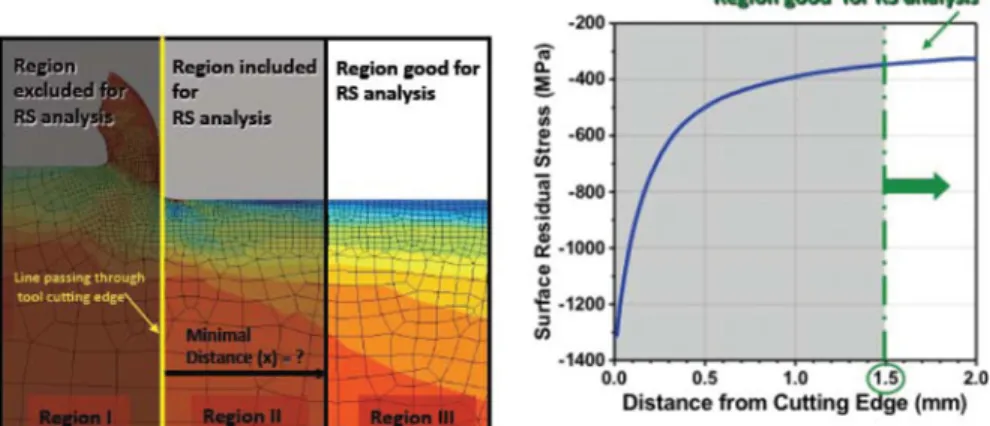
As explained by Outeiro et al. (2006a), if at the end of the simulation the chip is attached to the workpiece, the predicted residual stress components should be extracted from the model sufficiently far away from the chip formation zone. As shown in Figure 4, a strong residual stress variation is observed near the chip formation zone, which is not representative of the real residual stresses left in the workpiece. To avoid this zone, Region III should be selected to evaluate the residual stress components, being its distance from the chip root a function of the cutting conditions (cutting speed, feed, depth of cut, tool geometry/material, workpiece material, etc.).
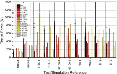
FIGURE 5 Simulated (color bars) and measured (black bar) cutting force values for different work
FIGURE 6 Simulated (color bars) and measured (black bar) thrust force values for different work materials and cutting conditions.
To compare both predicted and XDR-measured in-depth residual stress profiles, the predicted values need to be weighted using a function that takes into account the absorption of the X-ray in the materials under analysis, which can be calculated by the following equation:
⟨σR⟩ = *∞ 0 σ(z) · e− z/ τdz *∞ 0 e− z/ τdz (7)
where τ is the mean penetration depth of the X-ray beam in the material (Outeiro et al., 2013). Also, several residual stress profiles should be ex-tracted from the workpiece, covering a length equal to the length/diameter of the irradiated area in the machined surface. Then, an average residual stress value can be calculated for each depth.
COMPARISON OF THE RESULTS OBTAINED FROM DIFFERENT MODELS WITH EXPERIMENTAL DATA
Without the Calibration Procedure
The results are presented in Figures 5–9, where the measured and sim-ulated are represented by black and color bars, respectively. Figures 5 and 6 show the forces, Figure 7 shows the cutting temperatures (by definition is the maximum temperature at the tool-chip interface), Figure 8 shows the chip compression ratio, and Figure 9 shows the surface residual stress, σ //.
FIGURE 7 Simulated (color bars) and measured (black bars) cutting temperatures (the maximum temperature at the tool-chip interface) for different work materials and cutting conditions.
Figure 5 shows the predicted and measured cutting force for differ-ent work materials and simulation/test conditions. This figure also shows a higher dispersion of simulated cutting force for AISI 316L, IN 718 and
FIGURE 8 Simulated (color bars) and measured (black bar) Chip Compression Ratio (CCR), for
FIGURE 9 Simulated (color bars) and measured (black bar) surface residual stress σ //, for different work materials and cutting conditions.
Ti6AL4V work materials, and lower for AISI 1045 and AISI 52100 work ma-terials. As for the thrust force (Figure 6), except for the AISI 1045 steel, all the other work materials exhibit high dispersion. The differences in the cut-ting and thrust forces are greater than 90% for AISI 316L, AISI 52100, IN 718 and Ti6AL4V and for AISI 1045 steel, it is almost about 50%. As for the comparison between measured and simulated cutting and thrust forces, the best predictions were obtained for the AISI 1045.
Figure 7 shows the predicted and measured cutting temperatures for different work materials and simulation/test conditions. This figure shows a high dispersion between predicted cutting temperatures, and this dispersion is higher for AISI 316L, IN 718 and Ti6AL4V , and lower for AISI 1045. These results confirm what was previously observed for the cutting and thrust forces. Although the differences between the predicted cutting temperatures are lower when compared to the forces, these differences can reach 70-80% for AISI 316L, IN 718 and Ti6AL4V work materials, and a maximum of 30% for the AISI 1045. As for the comparison between measured and simulated cutting temperatures, the best predictions were obtained again for AISI 1045. It should be pointed out that since no experimental data on cutting temperatures was available for the AISI 52100 work material. Figure 8 shows the predicted and measured chip compression ratio (CCR) for different work materials and simulation/test conditions. This figure also shows a high dispersion among work materials. The differences in the CCR can reach 70% for AISI 316L and Ti6AL4V , and are slightly lower (about 50%) for the other work materials. As for the comparison between measured and
FIGURE 10 Dispersion of the simulated results of cutting force, cutting temperature, CCR and surface residual stress (SRS) acting in the circumferential direction (σ //).
simulated CCR, the best predictions were obtained for AISI 52100, and no experimental data was available for the AISI 1045 and AISI 316L work materials.
Residual stresses were measured in both cutting direction (σ //) and nor-mal to this direction (σ ⊥), but only the first stress component is presented in this manuscript, because it is the most critical one for the components’ functional performance and life in service. Figure 9 shows the predicted and measured surface residual stress, σ //, for different work materials and sim-ulation/test conditions. This figure shows a higher dispersion of simulated surface residual stress, σ //, for all work materials, and lower for AISI 52100, AISI 1045 and AISI 316L work materials, and higher for the other two work materials.
FIGURE 11 Simulated (color lines) and measured (black line) in-depth residual stress σ // profiles for
FIGURE 12 Simulated (color lines) and measured (black line) in-depth residual stress σ // profiles for the AISI 316L stainless steel.
In all cases, the differences between the predicted results are greater than 100%, being about 100%–140% for the AISI 52100, AISI 1045 and AISI 316L work materials, and more than 250% for the other two work materials. A significant difference between measured and simulated surface residual stress, σ //, is also observed, being the best predictions obtained for the AISI 1045 and AISI 52100 steels. Figure 10 shows the dispersion of the simulated results of cutting force, cutting temperature, CCR and surface residual stress (SRS) acting in the circumferential direction (σ //).
Looking into more details, the in-depth residual stress profiles (Fig-ures 11–15), it appears that this dispersion between simulated residual stresses is once again lower for the AISI 1045 steel and higher for AISI
FIGURE 13 Simulated (color lines) and measured (black line) in-depth residual stress σ // profiles for
FIGURE 14 Simulated (color lines) and measured (black line) in-depth residual stress σ // profiles for the Inconel 718 superalloy.
316L and IN 718 work materials. The best fits between measured and sim-ulated residual stresses were obtained for AISI 1045 steel, and partially for AISI 52100 and Ti-6Al-4V work materials.
In summary, in general, the results show a significant dispersion between simulated results. As shown in Figure 10, the smallest coefficient of variation, which is a normalized measure of dispersion of a distribution, is observed for the chip compression ratio, while the largest for surface residual stress, σ //. Moreover, the smallest dispersion was obtained for AISI 1045 and AISI 52100 steels, while the largest for AISI 316L, IN 718 and Ti6Al4V alloys. As far as the differences between measured and simulated results are concerned, they are also significant, being lower for AISI 1045, and in some cases for AISI 52100 and Ti-6Al-4V work materials. The worst predictions were obtained for AISI
FIGURE 15 Simulated (color lines) and measured (black line) in-depth residual stress σ // profiles for
316L and IN 718 work materials. The high dispersion between simulated results and their deviation in relation to the experimental results can be mainly attributed to different factors that the participants were free to setup on their own in their simulations. These are:
i) Numerical methods (FEM, Meshless), formulations (Lagrangian, ALE) and cor-responding parameters (element size, time step, etc.) and assumptions: A numer-ical model incorporates many numernumer-ical issues that are not easy to setup by someone who does not have sufficient knowledge about numerical methods. This is particularly evident for the software packages Abaqus, LS-Dyna, and to some extent, even Deform. For example, a simple selec-tion of the element size can strongly influence the model’s predicselec-tions. Moreover, any software package incorporates many assumptions that are not accessible by the users, but strongly affects the model’s predictions. ii) Boundary conditions (thermal and mechanical): The size of the geometrical model of the workpiece and tool, and how the thermal and mechan-ical boundary conditions are applied to this model can influence the temperature, stress and strains distributions, thus affecting the model’s predictive capability.
iii) Procedures for calculating the residual stresses and for extracting them from the model: There is no standard procedure to calculate and extract the resid-ual stresses from the model, and unfortunately, most of the scientific publications do not describe how they have done such calculations and extractions.
iv) Tool-chip and tool-work contact models and parameters (friction coefficient, fric-tion factor, heat transfer coefficient, etc.): The participants were free to select the contact models and the corresponding values of the model’s coeffi-cients. The friction coefficient is the most used parameter to describe the relationship between normal and contact stresses. As shown by in pre-vious publications (Astakhov, 2006; ¨Ozel and Ulutan, 2012; Rech et al., 2013), this coefficient is not constant along the tool-chip contact, and it depends on the contact conditions (contact pressure, sliding velocity and temperature). An incorrect determination/selection of the friction coefficient can strongly influence/affect the model’s predictions. v) Incorrect description of the mechanical behavior of the work material in
machin-ing: In particular, the incorrect description of the work material flow stress and fracture in metal cutting contributes to these differences. This is particularly critical for materials such as AISI 316L, IN718 and Ti6Al4V that exhibit low thermal conductivity and high strain hardening tendency. Such materials are prone to adiabatic shear banding result-ing in the formation of shear localized/segmented chips. Therefore, it is likely that the larger dispersion observed in terms of forces, temper-atures and residual stresses between the simulations and experiments for these materials may be related to how accurate is the description of
the work material flow stress and fracture to capture properly the cyclic nature of the chip formation process. Due to the high importance of this subject, this will be described in detail as follows.
As shown by Astakhov and Shvets (2004), the principal difference that exists between machining and all other metal forming processes is the phys-ical separation of the layer being removed (in the form of chips) from the rest of the workpiece. The process of physical separation of a solid body into two or more parts is known as fracture, and thus machining must be treated as the purposeful fracture of the layer being removed. Extensive work in this topic has also been reported by Atkins (2003). From this context, a proper modeling of the work material in machining should take into account not only the determination of the material flow stress under similar conditions as those observed in machining, but also under which conditions the fracture would occur and how to model it properly.
As far as the flow stress is concerned, the split Hopkinson pressure bar (SHPB) (Kolsky, 1949) is largely used to determine the work mate-rial flow stress under high strain-rates frequently encountered to metal cutting. Unfortunately, the SHPB has some drawbacks that can compro-mise the validity of the results, including the oscillations that flow stress exhibits particularly at low strains (Jaspers, 1999). Moreover, the flow stress depends on the strain path (Guo et al., 2005). According to Silva et al. (2012), the strain path induced by the SHPB is different from that found in metal cutting. Finally, the flow stress data is usually represented by the Johnson-Cook (JC) constitutive model (Johnson and Cook, 1983), available in most of the commercial FE codes, including those used in this benchmark study.
As mentioned by Guo and Horstemeyer (Guo et al., 2005), although this model is easy to apply and can describe the general response of material deformation, this model is deficient in the mechanisms to reflect the static and dynamic recovery, and the effects of load path and strain-rate history in large deformation processes, such as the case of metal cutting process. These effects are fundamental to properly modeling the surface integrity of machined components, including the residual stress distribution (Guo et al., 2005). Moreover, when presuming that no external heat source is added to the cutting process, the term on thermal softening of the JC constitutive model [see Equation (1)] is not necessary. In fact, the heat generated un-der high strain-rates accelerates the temperature rise and creates adiabatic localized regions in both mechanical tests for the characterization of the ma-terial flow stress and machining alike. Thus, the strain-hardening measured in high rate material testing may have included the thermal softening effects as well (Abushawashi et al., 2011).
As far as damage and fracture are concerned, they are essential to model chip formation (separation of the material from the workpiece to form the
chip), as well as, for chip segmentation. Therefore, a proper modeling of damage and fracture is essential and the corresponding models should con-sider both damage initiation, as well as damage evolution (Abushawashi et al., 2011; Mabrouki et al., 2008). In ductile materials, the damage initia-tion model should be established based on the material ductility, thus the equivalent strain at fracture. The equivalent strain at fracture is sensitive to the state of stress, being the stress triaxiality and the Lode angle two param-eters that affect this strain (Abushawashi et al., 2013; Bai and Wierzbicki, 2008).
In the case of plane-strain condition, which is the case for orthogonal cutting, the equivalent strain at facture is only affected by the stress triaxiality (Abushawashi et al., 2011). Increasing exigencies in terms of productivity leads to the application of h triaxiality igh cutting speeds (i.e., high speed machining), and consequently the work material is submitted to high strain-rates. Therefore, the strain-rate sensitivity to fracture must also be included in the fracture model as well. Concerning the temperature effects on the strain at fracture, what was mentioned above is also applied here. Therefore, a suitable model of damage initiation in orthogonal metal cutting should consider both stress triaxiality and strain-rate effects.
There are several fracture models that incorporate these effects, includ-ing the Johnson and Cook model (Johnson and Cook, 1983), and the Rice and Tracey fracture models (Rice and Tracey, 1969). The determination of the coefficients of these fracture models for a given work material re-quires resources and involves a series of experimental fracture tests (varying the stress triaxiality and strain-rate). Moreover, the implementation of such models in some FE codes can be more complex. For these reasons, in many metal cutting models, the fracture is ignored, because it is easier to model chip formation using non-physical criterion such as the remesh procedure.
In summary, modeling chip formation without a proper material model, that includes damage and fracture, results in unrealistic material behavior, where the material flow is somewhat unlimited with no material stiffness degradation. Moreover, the chip morphology (e.g., segmentation) obtained by such incomplete models produces an unrealistic smooth chip with unlim-ited material stretching and hardening (Abushawashi et al., 2013).
Applying the Calibration Procedure
The calibration procedure was developed and applied to four additional orthogonal cutting simulations performed on IN 718 and Ti-6Al-4V alloys (two simulations per work material). The objective here is to develop and calibrate new models based on the measured forces, chip geometry and chip compression ratio, and to apply them to predict the residual stresses. Figures 16–17 show that although a small improvement was seen in the near
FIGURE 16 Simulated (color lines) and measured (black line) in-depth residual stress σ // profiles, after applying the calibration procedure (Inconel 718).
surface residual stress for Ti-6Al-4V , no other relevant improvement was observed.
These results prove that the calibration procedure cannot improve the model’s “predictability” and a very important part of the solution for the problem is to consider a proper material model that includes not only flow stress, but also damage and fracture.
CONCLUSIONS AND OUTLOOK
A benchmark study was conducted to evaluate the effectiveness of the current numerical predictive models for machining performance. This study
FIGURE 17 Simulated (color lines) and measured (black line) in-depth residual stress σ // profiles,
includes collaboration of 22 international participants from universities, re-search institutes and companies and/or software developers from 10 coun-tries. Orthogonal cutting models for five work materials (AISI 1045, AISI 52100, AISI 316L, IN 718 and Ti-6Al-4V ) were developed and simulated using different commercial and non-commercial software packages (AN-SYS, Deform, LS-Dyna, AdvantEdge and a non-commercial software from the Yokohama National University), applying different numerical methods (FEM and Meshless) and formulations (Lagrangian, ALE). Predicted results (cutting and thrust forces, cutting temperatures, chip compression ratio and residual stresses) obtained from different participants were compared with those results obtained experimentally.
The predicted results clearly show a high dispersion among them, be-ing this dispersion higher for the residual stresses and lower for the chip compression ratio. Moreover, a higher dispersion of the results among work materials is generated for AISI 316L, IN 718 and Ti-6Al-4V work materials when compared with AISI 52100 and AISI 1045 steels. From the comparison between predicted and measured results, it is noted that the best predictions were obtained for AISI 1045, intermediate for AISI 52100 and Ti-6Al-4V work materials, and the worst for AISI 316L and IN 718 work materials. Thus, in general, the best uniformity among all predicted results and the best pre-dictability were obtained for the AISI 1045 work material.
Several factors will justify the obtained results, including incorrect de-scription of the work material behavior in metal cutting (flow stress and fracture) and of the tool-chip contact. In the case of residual stresses, they are very sensitive to the energy required for separating the material from the workpiece to form the chip (energy of plastic deformation and fracture). Therefore, an improper modeling of the flow stress and fracture in metal cutting simulations leads to a high dispersion among the simulated residual stress results. Moreover, the different approaches used by the participants of this study to “generate” the chip (remeshing technique, ALE formula-tion, sacrificial layer based on the fracture energy, etc.) also contribute to increasing differences in the predicted residual stress.
To improve the predictability of present metal cutting models, accurate modeling of the tool-chip contact and the work material behavior is required. In particular, new experimental tests need to be designed and developed for accurately characterizing the materials mechanical behavior. These experi-mental tests should reproduce the signature of the metal cutting process in terms of strain-rate and the state-of-stress. Moreover, Johnson-Cook model no longer serves the purpose of the metal cutting simulations, especially if residual stress (or surface integrity in general) is concerned. The develop-ment of physics-based models that takes into account the microstructural features is essential.
Inconsistent experimental metal cutting tests (including different acquisition techniques and their calibration) and incorrect comparison
between predicted and measured results (in particular the residual stresses) contribute to the observed differences between measured and predicted results. Therefore, a proper design of such experimental tests and the use of a suitable methodology to compare predicted and measured results would be required.
ACKNOWLEDGMENTS
The authors gratefully acknowledge the participation of the following researchers/institutions for performing numerical simulations and carrying out the experimental tests: Dr. C. Fischer, Scientific Forming Technologies Corp. (SFTC), USA; Dr. R. Ivester, National Institute of Standards and Tech-nology (NIST), USA; Dr. S. Rizzuti, Politecnico di Torino, Italy; Prof. A. Del Prete, University of Salento, Italy; Dr. N. Gramegna, Enginsoft, Italy; Prof. D. Biermann and Prof. B. Svendson, University of Dortmund, Germany; Prof. E. Ceretti, University of Brescia, Italy; Prof. C. Giardini, University di Bergamo, Italy; Prof. J. Rech, Ecole Nationale d’Ing´enieurs de Saint-Etienne (ENISE), France; Prof. J. Shinozuka, Yokohama National University, Japan; Prof. M. H. Attia, McGill University, Canada; Prof. J.P. Arrazola, University of Mondragon, Spain; Prof. T. Ozel, Rutgers University, USA; Prof. Y. Karpat, Bilkent University, Turkey; Prof. V. Schulze, Karlsruher Institut f¨ur Tech-nologie (KIT), Germany; Prof. T. Mabrouki and Dr. Y. Zhang, INSA-Lyon, France; Prof. K. Wegener, Dr. M. R¨othlin, Dr. N. R¨uttimann, IWF- ETH Zurich, Switzerland.
REFERENCES
Abushawashi, Y.; Xiao, X.; Astakhov, V. (2011) FEM simulation of metal cutting using a new approach to model chip formation. International Journal of Advances in Machining and Forming Operations, 3: 71–92.
Abushawashi, Y.; Xiao, X.; Astakhov, V. (2013) A novel approach for determining material constitutive parameters for a wide range of triaxiality under plane strain loading conditions. International Journal
of Mechanical Sciences, 74: 133–142.
Altintas¸, Y.; Budak, E. (1995) Analytical prediction of stability lobes in milling. CIRP Annals - Manufacturing
Technology, 44: 357–362.
Arrazola, P.J.; ¨Ozel, T. (2010) Investigations on the effects of friction modeling in finite element simula-tion of machining. Internasimula-tional Journal of Mechanical Sciences, 52(1): 31–42.
Arrazola, P.J.; ¨Ozel, T.; Umbrello, D.; Davies, M.; Jawahir, I.S. (2013) Recent advances in modelling of metal machining processes. CIRP Annals - Manufacturing Technology, 62(2): 695–718.
Astakhov, V.P. (2006) Tribology of Metal Cutting. Elsevier, London.
Astakhov, V.P.; Outeiro, J.C. (2005) Modeling of the contact stress distribution at the tool-chip interface.
Machining Science and Technology: An International Journal, 9: 85–99.
Astakhov, V.P.; Outeiro, J.C. (2008) Metal cutting mechanics, finite element modelling. In: Davim, J.P. (Editor), Machining: Fundamentals and Recent Advances. Springer, New York.
Astakhov, V.P.; Shvets, S. (2004) The assessment of plastic deformation in metal cutting. Journal of
Materials Processing Technology, 146: 193–202.
Athavale, S.M.; Strenkowski, J.S. (1998) Finite element modelling of machining: from proof-of-concept to engineering applications. Machining Science and Technology: An International Journal, 2(2): 317–342.
Atkins, A.G. (2003) Modelling metal cutting using modern ductile fracture mechanics: quantitative ex-planations for some longstanding problems. International Journal of Mechanical Sciences, 45: 373–396. Attanasio, A.; Ceretti, E.; Rizzuti, S.; Umbrello, D.; Micari, F. (2008) 3D finite element analysis of tool
wear in machining. CIRP Annals - Manufacturing Technology, 57(1): 61–64.
Bai, Y.; Wierzbicki, T. (2008) A new model of metal plasticity and fracture with pressure and Lode dependence. International Journal of Plasticity, 24: 1071–1096.
Childs, T.H.C.; Maekawa, K.; Obikawa, T.; Yamane, Y. (2000) Metal Machining: Theory and Applications, Elsevier.
Cockroft, M.G.; Latham, D.J. (1968) Ductility and workability of metals. Journal of the Institute of Metals, 96: 33–39.
Dirikolu, M.H.; Childs, T.H.C.; Maekawa, K. (2001) Finite element simulation of chip flow in metal machining. International Journal of Mechanical Sciences, 43:2699–2713.
Filice L.; Micari, F.; Rizzuti, S.; Umbrello, D. (2008) Dependence of machining simulation effectiveness on material and friction modelling. Machining Science and Technology: An International Journal, 12/3: 370–389.
Fleischer, J.; Schmidt, J.; Xie, L.J.; Schmidt, C.; Biesinger, F. (2004) 2D tool wear estimation using finite element method. Proc. of the 7th CIRP International Workshop on Modeling of Machining Operations, Cluny, France 82–91.
Guo, Y.B.; Liu, C.R. (2002) FEM analysis of mechanical state on sequentially machined surfaces. Machining
Science and Technology, 6: 21–41.
Guo, Y.B.; Wen, Q.; Horstemeyer, M.F. (2005) An internal state variable plasticity-based approach to determine dynamic loading history effects on material property in manufacturing processes.
Inter-national Journal of Mechanical Sciences, 47: 1423–1441.
Huang, J.M.; Black, J.T. (1996) An evaluation of chip separation criteria for the fem simulation of machining. Journal of Manufacturing Science and Engineering, 118: 545–554.
Jaspers, S. (1999) Metal Cutting Mechanics and Material Behaviour (Ph.D), Technische Universiteit Eind-hoven.
Jawahir, I.S.; Brinksmeier, E.; M’Saoubi, R.; Aspinwall, D.K.; Outeiro, J.C.; Meyer, D.; Umbrello, D.; Jayal, A.D. (2011) Surface integrity in material removal processes: Recent advances. CIRP Annals
-Manufacturing Technology, 60(2): 603–626.
Johnson, G.R.; Cook, W.H. (1983) Fracture Characteristics of Three Metals Subjected to Various Strains, Strain Rates, Temperatures and Pressures. Engineering Fracture Mechanics, 21(1): 31–48.
Kolsky, H. (1949) An investigation of the material properties of materials at very high rates of loading.
Proceedings of the Physical Society. Section B, 62(11): 676–700.
Liu, M.; Takagi, J.; Tsukuda, A. (2004) Effect of tool nose radius and tool wear on residual stress distribution in hard turning of bearing steel. Journal of Materials Processing Technology, 150: 234–241. M’Saoubi, R.; Outeiro, J.C.; Inal, K.; Lebrun, J.L.; Dias, A.M. (1997) Residual stress and texture analysis in
machined surfaces of AISI 316Lsteels, in: T. Ericsson, M. Od´en, A. Andersson (Eds.), Presented at the Proceedings of The Fifth International Conference on Residual Stresses - ICRS5, pp. 349–354.
Mabrouki, T.; Girardin, F.; Asad, M.; Rigal, J.-F. (2008) Numerical and experimental study of dry cutting for an aeronautic aluminium alloy (A2024-T351). International Journal of Machine Tools and
Manufac-ture, 48: 1187–1197.
Marques, M.J.; Outeiro, J.C.; Dias, A.M.; M’Saoubi, R.; Chandrasekaran, H. (2006) Surface integraty of H13 ERS mould steel milled by carbide and CBN tools. Materials Science Forum, 514–516: 564–568. Movahhedy, M.; Gadala, M.S.; Altintas, Y. (2000) Simulation of the orthogonal metal cutting process using
an arbitrary Lagrangian-Eulerian finite-element method. Journal of Materials Processing Technology, 103: 267–275.
Outeiro, J.C.; Ee, K.C.; Dillon Jr., O.W.; Wanigarathne, P.C.; Jawahir, I.S. (2006a) Some observations on comparing the modelled and measured residual stresses on the machined surface induced by orthogonal cutting of AISI 316L steel, in: I. Grabec, E.G. (Editor), Presented at the 9th CIRP
Interna-tional Workshop on Modeling of Machining Operations, University of Ljubljana, Faculty of Mechanical
Engineering, pp. 475–481.
Outeiro, J.C.; Kandibanda, R.; Pina, J.C.Dillon Jr., O.W.; Jawahir, I.S. (2010) Size-effects and surface in-tegrity in machining and their influence on product sustainability. International Journal of Sustainable