Kinetic Analysis of Tropical Lignocellulosic Agrowaste Pyrolysis

HAL Id: hal-01581811

https://hal-mines-albi.archives-ouvertes.fr/hal-01581811

Submitted on 7 Nov 2019

HAL is a multi-disciplinary open access

archive for the deposit and dissemination of

sci-entific research documents, whether they are

pub-lished or not. The documents may come from

teaching and research institutions in France or

abroad, or from public or private research centers.

L’archive ouverte pluridisciplinaire HAL, est

destinée au dépôt et à la diffusion de documents

scientifiques de niveau recherche, publiés ou non,

émanant des établissements d’enseignement et de

recherche français ou étrangers, des laboratoires

publics ou privés.

Kinetic Analysis of Tropical Lignocellulosic Agrowaste

Pyrolysis

Lina Maria Romero Millan, Fabio Emiro Sierra Vargas, Ange Nzihou

To cite this version:

Lina Maria Romero Millan, Fabio Emiro Sierra Vargas, Ange Nzihou. Kinetic Analysis of

Trop-ical Lignocellulosic Agrowaste Pyrolysis.

BIOENERGY RESEARCH, 2017, 10 (3), pp.832-845.

Kinetic Analysis of Tropical Lignocellulosic Agrowaste Pyrolysis

Lina María Romero Millán1,2 _{&Fabio Emiro Sierra Vargas}1_{&Ange Nzihou}2

Abstract The thermal behavior of three Colombian agricul-tural residues was studied by non-isothermal thermogravimet-ric analysis (TGA) at various heating rates. An approach using a combined kinetics parallel reaction model and model-free isoconversional methods proved to be suitable to determine the pyrolysis kinetic parameters of biomasses with different macromolecular composition and H/C and O/C ratios near 1.5 and 0.8, respectively. Fraser-Suzuki functions representing the derivative TGA (DTG) of hemicellulose, cellulose and lignin showed a very good agreement with the experimental data. The calculated apparent activation energy of biomass pseudo-components evidenced no dependence on the reaction extent in all the conversion range, validating the use of master plots for decomposition mechanism identification. Pseudo-hemi-cellulose, pseudo-Pseudo-hemi-cellulose, and pseudo-lignin showed to be close to a second-order kinetic model, a random scission, or an Avrami-Erofeev model and a high-order kinetic model, re-spectively. Comparing the three feedstocks, the apparent acti-vation energy of the pseudo-components was in the order: bamboo guadua Ea< coconut shells Ea< oil palm shells Ea.

The results show that even when sample elemental composi-tion is very similar, macromolecular constituents, in particular lignin, could have an impact in the biomass decomposition rate and apparent activation energy. For the three studied ma-terials, the model fitting error below 10% showed that the

calculated kinetic parameters are suitable for the description and prediction of the biomass thermal decomposition. Keywords Kinetic modeling . Parallel reaction model . Pyrolysis . Lignocellulosic biomass . Thermogravimetric analysis

Nomenclature

α Degree of conversion or reaction extent (−) A Frequency factor or pre-exponential factor (min−1)

β Experiment heating rate (°C/min)

BG Bamboo guadua

ci Fraction of each i biomass pseudo-component

CS Coconut shells

dα/dt Decomposition rate (−)

daf Dry ash free

Ea Activation energy (kJ/mol)

OPS Oil palm shells

R Ideal gas constant 8.3144 J/mol K

t Time (min)

T Temperature (°C, K)

Introduction

Thanks to their climate variety, tropical regions have a great biodiversity and the appropriate conditions for the develop-ment of agroindustrial activities. Agroindustry produces large amounts of low-cost residues, which can be used for biofuel production or transformed in value-added products. However, in most tropical developing countries, these residues are not valorized and represent an environmental risk, as they are not always disposed properly. According to different studies, the agro-residues potential in developing countries is higher than

* Lina María Romero Millán

lmromerom@unal.edu.co; lina.romero_millan@mines-albi.fr

1 _{Facultad de Ingeniería, Ciudad Universitaria, Universidad Nacional}

de Colombia–Sede Bogotá, Bogotá, Colombia

2 _{Université de Toulouse, Mines Albi, CNRS, Centre RAPSODEE,}

2900 million t per year [1]. In Colombia, according to the Colombian Energy and Mining Planning Unit, UPME, more than 70 million t of wastes is produced every year from agroindustrial activities [2]. In this context, the valorization of these residues from an energetic point of view or for the production of value-added products represents an alternative for their treatment and disposal and for strengthening the local economy.

Three Colombian lignocellulosic biomasses were chosen for this study: oil palm shells (OPS), coconut shells (CS), and bamboo guadua (BG). OPS are the shell fractions left after the crushing of the kernel nut in the oil palm extraction pro-cess from the Elaeis guineensis palm. This biomass is consid-ered an important waste of the Colombian oil palm extraction industry, with near 220,000 t generated every year [2]. In the country, raw OPS are usually burnt in boilers for steam pro-duction in palm oil facilities, or disposed as a cover for palm plantation roads, without giving any value to this residue [3]. Furthermore, CS from Cocos nucifera palm are considered a material with little or non-economic value from the Colombian alimentary industry, and have been traditionally used for handicraft making or discharged in soils. The amount of this residue is not negligible in the country, considering that near 119,000 t of this fruit is produced in Colombia every year, according to the statistics from the Food and Agriculture Organization of the United Nations [4]. Finally, BG, Guadua angustifolia Kunth, is a native woody bamboo spe-cies from South and Central America [5,6]. It has been tradi-tionally used in Colombia as a construction material or fire-wood. With a high growing rate, BG could represent an inter-esting material for energy purposes in Colombia and other tropical countries, either from crops or as a residue from the construction industry. Energetic applications of this biomass have not been studied in detail. Reported studies related to bamboo as energy source have been mainly performed with other bamboo species [7–9]. Considering that the three select-ed biomasses have a heating value above 18 MJ/kg and a great availability [5,10,11], it could be interesting to explore their potential to be used as a source of energy, or as a feedstock for the production of value-added materials in Colombia and oth-er tropical countries.

Pyrolysis is the first step in the conversion of biomass into biofuels, adsorbent materials, and value-added chemicals [12–15]. This thermochemical conversion process constitutes the previous stage of combustion and gasification, and should be properly understood for the valorization of different mate-rials through thermochemical conversion processes. In partic-ular, the knowledge of the pyrolysis kinetic parameters is very important to analyze the thermal decomposition process of residual biomasses, predict their conversion, and determine their possible valorization pathways.

Thermogravimetric analysis (TGA) has been widely used for the study of lignocellulosic biomass decomposition

kinetics, either from isothermal and non-isothermal ap-proaches. Several pyrolysis kinetic studies using non-isothermal data have focused on model-free methods to esti-mate the biomass kinetic parameters, as they allow the evalu-ation of the activevalu-ation energy without knowing the decompo-sition reaction model [16,17]. However, considering that the biomass pyrolysis is an extremely complex process due to the morphologies of its components and their interaction, the model-free procedure is not always sufficient for the identifi-cation of the complete kinetic triplet [18]. Most biomass py-rolysis analysis has reported different activation energy values for several kinds of lignocellulosic biomasses, usually consid-ering only a global decomposition approach [19–22]. Works based on model-free isoconversional methods, showed that there is a clear dependence of activation energy on the reaction extent, suggesting that the pyrolysis process includes many different reactions occurring at the same time. Under these circumstances, an interesting alternative for the analysis of complex conversions is a parallel reaction approach, separat-ing the individual processes by derivative TGA (DTG) peak deconvolution [23], followed by the kinetic analysis of the resulting individual curves. Few studies have been reported for biomass pyrolysis kinetic analysis using DTG deconvolution [24–26]. In particular, BG, CS, and OPS kinet-ic analysis using this alternative approach has not been report-ed yet.

According to this, the aim of this work is to study the pyrolysis characteristics and kinetics of three tropical ligno-cellulosic biomasses, from a non-isothermal TGA. A three-parallel reaction model was employed, using a DTG peak deconvolution procedure, followed by a model-free isoconversional approach and generalized master plots. The influence of the biomass nature in its thermal decomposition characteristics was discussed, comparing the calculated kinet-ic parameters of the selected materials.

Materials and Methods

Tropical feedstocks used in this study were collected in Colombia, South America. OPS were provided by a palm oil extraction plant in the Meta region (4° 16′ 00″ N 73° 29′ 00″ O, 500 m above sea level, average temperature 27 °C and 2858 mm of precipitation throughout the year). CS from co-conuts coming from the Nariño region (1° 10′ 00″ N 77° 16′ 00″ O, 0 to 400 m above the sea level and 28 °C of average temperature) were provided by a food processing industry. Both OPS and CS are considered as an industrial residue. For its part, 3- to 4-years-old BG coming from a bamboo forest in the Quindío region (4° 32′ 00″ N 75° 42′ 00″ O, 800 to 1200 m above sea level and 23 °C of average

temperature) was obtained from a furniture and handicraft construction site, where biomass was indoor stored.

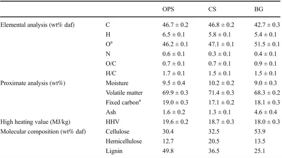
Raw materials were milled and sieved to a size range of 1 to 2 mm before TGA. CHNS composition of samples was deter-mined using a Themoquest NA 2000 elemental analyzer. Moisture, volatiles, and ash content were calculated according to the standards EN ISO 18134-3, EN ISO 18123, and EN ISO 18122, respectively. The high heating value was calculat-ed using an IKA C 5000 automatcalculat-ed bomb calorimeter. The sample chemical composition and heating value are presented in Table1as an average of three replicates. Molecular com-position of the biomasses is referred to literature reported values [27–29].

Thermogravimetric Analysis

Thermogravimetric analysis (TGA) of selected materials was performed using a Mettler Toledo TGA 2 SF analyzer. Approximately 30 mg of each sample was placed in an alu-mina crucible and heated from 25 to 800 °C, with 2, 5, 10, and 20 °C/min as heating rates. Experiments were conducted un-der a nitrogen atmosphere, using a flow rate of 50 ml/min. To verify the repeatability of TGA experiments, each run was conducted two times and averaged; then, the mean standard deviation was calculated. A blank experiment was made for each heating rate to exclude buoyancy effects. Experimental runs were first performed at 2 °C/min, followed by 5, 10, and 20 °C/min. Duplicates were done following the same order described. For each experimental condition, the standard de-viation was below 0.6% for the investigated temperature range. This value was considered reasonable to ensure the repeatability of the obtained mass loss curves.

Kinetic Study

Theoretical Background

TGA has been extensively used to study the kinetics of bio-mass pyrolysis and to determine the reaction mechanisms con-trolling this process. Generally, the basis of a kinetic study is a series of experiments where the degree of conversion of a material is measured as a function of time and temperature. According to this, the degree of conversion or reaction extent is usually defined as in Eq. (1).

α ¼ _mm0−m

0−mf ð1Þ

where m0is the initial mass of the sample, mfthe final mass,

and m the current mass at a given temperature or time. The reaction rate dα/dt depends on the temperature T and the de-gree of conversion α, as shown in Eq. (2). In this expression, f(α) is the reaction model function representing how the

solid-state decomposition process occurs, and k(T) the Arrhenius equation, representing the temperature dependence of the pro-cess. dα dt ¼k Tð Þf αð Þ ð2Þ k T_{ð Þ ¼ A exp} −Ea RT ! " ð3Þ From the Arrhenius equation (Eq. (3)), the reaction rate expression can be rearranged as follows:

dα dt ¼A exp −Ea RT ! " f αð Þ ð4Þ

Finally, for linear non-isothermal TGA, the reaction rate is expressed as in Eq. 5, where β is the heating rate used to perform the experiment in Kelvin per min.

dα dT ¼ A β exp −Ea RT ! " f α_{ð Þ ð5Þ}

In the case of biomass decomposition, the most commonly accepted reaction model functions f(α) and their integral forms are presented in Table2.

Three-Parallel Reaction Model

Thermal decomposition of lignocellulosic biomass is quite complex, considering that it is constituted by different com-ponents, mainly hemicellulose, cellulose, and lignin. Accordingly, pyrolysis can be described with a parallel reac-tion model (PRM), assuming that the three main components of the biomass react independently [31]. Three pseudo-components representing the hemicellulose, cellulose and lig-nin are then considered in this approach. The total reaction rate is expressed as the addition of each pseudo-component reac-tion rate, as in Eq.6.

dα dT ¼ ∑ 3 i¼1ci dαi dT ð6Þ

It is important to note that modeled pseudo-components do not represent the real proportion of biomass constituents, as interactions between them can exist [32]. However, the pseudo-component proportion should be in accordance with each biomass molecular composition.

In order to model these three parallel reactions, the biomass DTG curves were deconvoluted, representing each pseudo-component reaction rate as a mathematical function of tem-perature. Global DTG curves were then considered as the addition or overlap of pseudo-component DTG profile. Gaussian, Lorentzian, and Fraser-Suzuki functions were used in this study.

Gaussian function [26]: dα dT ! " i¼ a exp − 1 2 T−b c ! "2 " # ð7Þ where a is the amplitude in 1/K, bis the peak temperature in K, and c is the width of the curve in K.

Lorentzian function [26]: dα dT ! " i¼ a 1 þ T−bc # $2 ð8Þ

where a is the amplitude in 1/K, bis the peak temperature in K, and c is the width of the curve in K.

Fraser-Suzuki function [33]: dα dT ! " i¼ a exp − ln2 d2 ln 1 þ 2d T−b c ! " % &2 ( ) ð9Þ

where a is the amplitude in 1/K, bis the peak temperature in K, c is the half width of the curve in K, and d is the asymmetry of the curve.

Least square method and an optimization algorithm were used to determine the function parameters that best fit each biomass experimental decomposition profile. The fit error was determined with Eq.10, where dα/dT are the experimental and

Table 2 Most common reaction mechanisms used in solid-state kinetic analysis related to biomass thermal decomposition

Model f(α) g(α)

Order based Or1, first order 1− α −ln(1 − α) Or2, second order (1− α)2 _{[1/(1− α)] − 1}

Or3, third order (1− α)3 _{[1/(1− α)}2_{]− 1}

Diffusion D1, one dimensional 1/(2α) α2

D2, two dimensional [−ln(1 − α)]−1 _{α + (1− α)ln(1 − α)}

D3, three dimensional (3/2)(1− α)2/3_{[1− (1 − α)}1/3_]−1 _{[1− (1 − α)}1/3_]2

D5, three dimensional (3/2)(1− α)4/3_{[(1− α)}−1/3_–1]−1 _{[(1− α)}−1/3_{− 1]}2

Power law Pn, power law α1/2 _n(α)(n− 1)/n

Nucleation and growth An, Avrami-Erofeev [−ln(1 − α)]1/n _{n(1− α)[−ln(1 − α)]}(n− 1)/n

Geometrical contraction R2, Contracting area 2(1− α)1/2 _{1− (1 − α)}1/2

R3, Contracting volume 3(1− α)2/3 _{1− (1 − α)}1/3

Random scission L2, Random scission L = 2 2(α1/2_{− α) –}

Source: [18,30]

Table 1 Heating value and chemical composition of studied biomasses

OPS CS BG

Elemental analysis (wt% daf) C 46.7 ± 0.2 46.8 ± 0.2 42.7 ± 0.3 H 6.5 ± 0.1 5.8 ± 0.1 5.4 ± 0.1 Oa _{46.2 ± 0.1 47.1 ± 0.1 51.5 ± 0.1}

N 0.6 ± 0.1 0.3 ± 0.1 0.4 ± 0.1 O/C 0.7 ± 0.1 0.7 ± 0.1 0.9 ± 0.1 H/C 1.7 ± 0.1 1.5 ± 0.1 1.5 ± 0.1 Proximate analysis (wt%) Moisture 9.5 ± 0.4 10.2 ± 0.2 9.0 ± 0.3 Volatile matter 69.9 ± 0.3 71.4 ± 0.3 68.3 ± 0.2 Fixed carbona _{19.0 ± 0.3 17.1 ± 0.2 18.1 ± 0.3}

Ash 1.6 ± 0.2 1.3 ± 0.1 4.6 ± 0.4 High heating value (MJ/kg) HHV 19.6 ± 0.2 18.7 ± 0.3 18.0 ± 0.3 Molecular composition (wt% daf) Cellulose 30.4 32.5 53.9

Hemicellulose 12.7 20.5 13.5 Lignin 49.8 36.5 25.1

calculated values of the decomposition rate, and N is the total number of experimental points [32]. According to this, the smaller the fit error, the better fit to the experimental data.

Fit error %ð Þ ¼ 100 ffiffiffiffiffiffiffiffiffiffiffiffiffiffiffiffiffiffiffiffiffiffiffiffiffiffiffiffiffiffiffiffiffiffiffiffiffiffiffiffiffiffiffiffiffiffiffiffiffi ∑N i¼1 dαdTi # $ exp− dαdTi # $ calc ( )2 r ffiffiffiffi N p # $ dαi dT # $ exp;max 0 B B @ 1 C C A ð10Þ

Once the best fit was determined, isoconversional model-free methods were used for kinetic analysis, as presented in BIsoconversional Model-Free Approach^ section.

Isoconversional Model-Free Approach

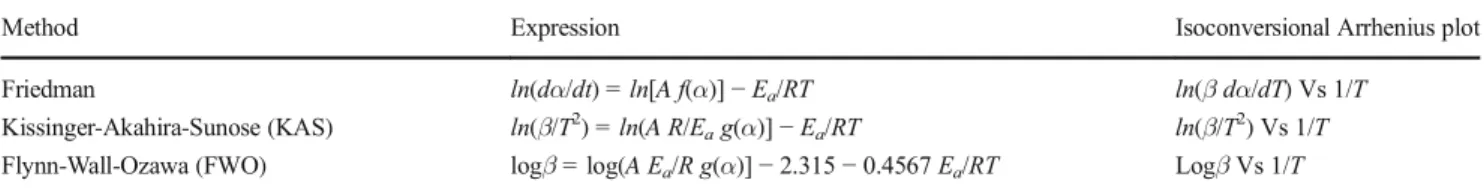
In this study, different isoconversional model-free methods were used to determine the Arrhenius parameters from exper-iments performed with four different heating rates. In particu-lar, three isoconversional methods were compared: Friedman, Flynn-Wall-Ozawa (FWO), and Kissinger-Akahira-Sunose (KAS). Friedman is defined as a differential method, while FWO and KAS are integral methods [18, 34]. All of them are well known and widely used for thermal decomposition kinetic analysis. The activation energy value at a constant α can be calculated from the slope of the isoconversional Arrhenius plots, according to the expressions summarized in Table3.

If the apparent value of Eadoes not vary in a significant

way with α, the process can be described by a single-step kinetics, and then, generalized master plots can be used to determine the most suitable reaction mechanism associated and, as a result, the pre-exponential factor A. The reduced-generalized reaction rate expression in Eq.11needs the pre-vious knowledge of activation energy value [35].

λ α_{ð Þ ¼} f αð Þ f α_{ð Þα¼0:5} ¼ dα=dt dα=dt ð Þ0:5 exp Eð a=RTÞ exp Eð a=RT0:5Þ ð11Þ

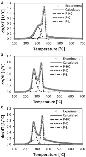
The most suitable f(α) model can be identified as the best match between the experimental λ(α) values and the theoret-ical master plots presented in Fig.1[36].

Results and Discussion

Biomass Composition and Thermal Decomposition Characteristics

In reference to the biomass chemical composition presented in Table1, it is possible to observe that the three selected mate-rials have similar C and H contents, with H/C ratio between 1.5 and 1.7. In contrast, the molecular composition has re-markable differences, particularly related to lignin content. OPS and CS are endocarp biomasses with relatively high

lignin content (50 and 36%, respectively). In contrast, BG has lignin content below 25% and a high proportion of cellu-lose (>50%).

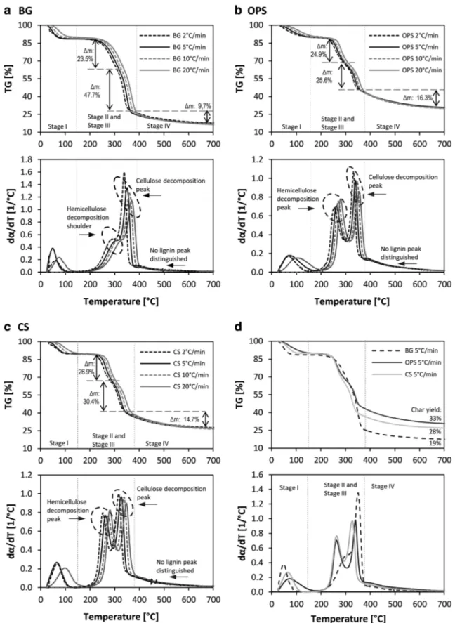
Regarding the thermal decomposition behavior, the TG and DTG curves of biomasses are presented in Fig.2. For the three samples, it is possible to distinguish four decomposition stages. The first one (stage I), registered before 200 °C, is related to the moisture and light volatile release. The second and the third one (stage II and stage III), from 200 to 330 °C and from 300 to 380 °C, correspond mainly to the hemicellu-lose and celluhemicellu-lose decomposition, and the last one (stage IV), from 380 °C, is mainly related to lignin decomposition. These decomposition ranges found are in accordance with reported values for cellulose, hemicellulose, lignin, and other lignocel-lulosic biomasses [12,37].

It is possible to notice from the TG curves that the mass loss in each stage is in agreement with the fraction of hemicellu-lose, celluhemicellu-lose, and lignin of the samples. In a dry basis, the three biomasses, with similar hemicellulose content, showed a similar mass loss during the second decomposition stage. This value, higher than their reported hemicellulose composition, was expected, taking into account that during this stage, some light volatiles can also be released. Regarding the third stage, BG showed the greatest mass loss, in accordance with its high cellulose content (53.9%). In the same way, the comparison of the TG curves, presented in Fig.2d, showed that the char yield at the end of the test was different for each biomass. OPS solid residue was 33%, while CS and BG solid yield was 28 and 19%, respectively. These differences could be related to the molecular composition of the samples. It is known that lignin contributes in an important way to the solid yield in biomass decomposition [12], explaining the fact that OPS, with the highest lignin content, registered the lowest mass loss, follow-ed by CS and BG.

Moreover, significant differences can be observed between the DTG curves. In the case of OPS and CS, two distinct peaks can be identified for hemicellulose and cellulose decomposi-tion; while for BG, the hemicellulose decomposition is repre-sented by a shoulder next to the cellulose peak. It should also be noted that as lignin decomposition range occurs over a wide temperature range from 150 to 800 °C [38], no specific lignin peak could be distinguished. Regarding the cellulose decomposition rate, endocarp biomasses showed lower values compared with BG. Taking into account that lignin is the binding agent of biomass fibers, higher lignin contents could be related to lower cellulose decomposition rates and with the well-differentiated decomposition peaks for hemicellulose and cellulose. In relation to this, Lui et al. [39], studied the interaction between biomass components during pyrolysis. They concluded that lignin has a strong effect in hemicellulose and cellulose decomposition. Mendu et al. [40] also found that high lignin biomasses show well-differentiated peaks for hemicellulose and cellulose decomposition.

DTG Curve Deconvolution

Biomass DTG curves were deconvoluted, representing each pseudo-component with Gaussian, Lorentzian, and Fraser Suzuki functions. As Gaussian and Lorentzian functions are symmetric, they were particularly inadequate to fit the OPS and CS decomposition patterns, with an error greater than 13 and 15%, respectively. In contrast, Fraser-Suzuki function allowed the fitting of asymmetric curves, giving a good agree-ment with experiagree-mental data. In all cases, the fit error was lower than 3%. Parejon et al. [23] found that Fraser-Suzuki function is the mathematical algorithm that better fits the de-composition rate patterns of complex processes. Figure3 pre-sents the results of the Fraser-Suzuki deconvolution fitting of BG, CS, and OPS at a heating rate of 10 °C/min. Table 4

summarizes the final parameters that better fitted each exper-imental data set.

From the deconvolution results, the pseudo-hemicellulose, pseudo-cellulose, and pseudo-lignin fractions of biomass sam-ples were calculated. BG values were 32, 49, and 19%, re-spectively. CS values were 28, 29. and 42%, and finally, OPS values were 26, 24, and 50%. It should be noted that even when modeled pseudo-components do not represent the real proportion of biomass constituents, their fractions show the different nature of the studied samples in terms of their mo-lecular composition.

Kinetic Analysis

For the selected biomasses, decomposition rate curves (dα/ dT Vs T) of each pseudo-component were analyzed using isoconversional model-free methods, in order to determine their kinetic triplet Ea, A, and f(α). Friedman, KAS, and

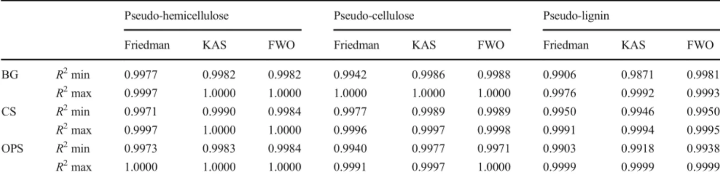
FWO Arrhenius plots for OPS, CS, and BG pseudo-components showed a good linear fit in all the conversion range between 0.1 and 0.9. In all cases, R2 values were higher than 0.9871, as presented in Table 5, where the

maximum and minimum R2 _{values are summarized. The}

high correlation coefficients R2 obtained suggest that the three isoconversional methods used are reliable and accu-rate for the apparent activation energy calculation.

Biomass pseudo-component Eawas determined from the

slope of the isoconversional plot regression lines, according to the Friedman, KAS, and FWO methods, presented in Table3. The calculated Eavalues are shown in Fig.4, as a function of

the reaction extent.

It is possible to observe that in all cases, the dependence of Eaon α is quite low. The apparent activation energy remained

almost constant in all the conversion range, indicating that pseudo-component thermal decomposition follows a single-stage process and no complex reactions occur [30]. In relation to this, Table6summarizes the mean activation energy value found for the three biomass pseudo-components, using the described isoconversional methods. It should be noted that the relative standard deviation of the activation energy was always lower than 8% (σ = 13.5 kJ/mol), with values even below 2% (σ = 3.2 kJ/mol).

Friedman, KAS, and FWO approaches gave similar appar-ent activation energy values with absolute deviation below 11% in all cases. These results show that all the three methods are convenient for the calculation of the activation energy of the sample pseudo-component decomposition. In particular, it can be said that for biomasses with H/C and O/C near 1.6 and 0.8, any of the presented methods is suitable for the determi-nation of pyrolysis kinetic parameters, despite the differences in hemicellulose, cellulose, and lignin fractions and their de-composition behavior.

The highest absolute deviation between the methods was found for the mean Eacalculated with Friedman and FWO for

OPS pseudo-hemicellulose (22.4 kJ/mol—10.5%). In con-trast, the results obtained with KAS and FWO were very close, with deviations below 1%. These differences are related

Table 3 Kinetic model-free methods used in this study

Method Expression Isoconversional Arrhenius plot Friedman ln(dα/dt) = ln[A f(α)]− Ea/RT ln(β dα/dT) Vs 1/T

Kissinger-Akahira-Sunose (KAS) ln(β/T2_{) = ln(A R/E}

ag(α)]− Ea/RT ln(β/T2) Vs 1/T

Flynn-Wall-Ozawa (FWO) logβ = log(A Ea/R g(α)]− 2.315 − 0.4567 Ea/RT Logβ Vs 1/T

0 1 2 3 4 0.0 0.2 0.4 0.6 0.8 1.0 λ( α) α [%] Or1 Or2 Or3 P4 A1,5 A2 A3 L2 R2

Fig. 1 Generalized master plots of the different kinetic models in Table2, constructed according to Eq.6

to the mathematical approach of the isoconversional methods and the treatment of the experimental data, considering that

Friedman is a differential method while FWO and KAS are integral.

Fig. 2 TG and DTG curves at 2, 5, 10, and 20 °C/min. a Guadua angustifolia Bamboo guadua (BG). b Oil palm shells (OPS). c Coconut shells (CS). d Comparison of TG and DTG curves at 5 °C/min. Mass loss values and char yield are presented in a dry basis

From Table6, it is also possible to notice that for the three biomasses, pseudo-component decomposition followed near-ly the same behavior, as Ea is in the order: Ea

pseudo-hemicellulose < Ea pseudo-cellulose < Ea pseudo-lignin.

Keeping in mind that Eais the minimum energy required to

start a reaction, the lower pseudo-hemicellulose Ea value

means that this component degrades easier than the two others. Accordingly, it is possible to see from Fig. 4 that pseudo-hemicellulose decomposition starts at a lower temper-ature than that of pseudo-cellulose and pseudo-lignin. For its part, pseudo-lignin decomposition over a large temperature range indicates that this component degrades slowly, and is

harder to decompose than hemicellulose and pseudo-cellulose. The high Eavalues associated with pseudo-lignin

could be related to its aromatic nature and the fact that this component is the cementing agent of biomass fibers. Lignin is a complex three-dimensional polymer with a large variety of chemical functions which differ in thermal stability and de-compose in a broad temperature range [41], interacting with cellulose and hemicellulose. These interactions during bio-mass decomposition may explain the fact that calculated pseudo-lignin activation energy is higher than isolated lignin reported values, which can be in the range of 37 to 160 kJ/mol, depending on the analyzed lignin type [42,43].

Table 4 Fitting results of Fraser-Suzuki deconvolution of selected biomasses

BG CS OPS Parameters P-HC P-C P-L P-HC P-C P-L P-HC P-C P-L 2 °C/min a (1/K) −0.450 −1.460 −0.110 −0.620 −0.795 −0.169 −0.520 −0.840 −0.220 b (°K) 283.0 337.7 359.0 251.0 315.0 293.0 251.5 328.5 301.0 c (°K) 57.0 23.0 180.0 36.5 26.0 175.0 35.8 20.5 182.0 d (−) −0.200 −0.420 0.210 0.350 −0.300 0.555 0.360 −0.400 0.630 Fit error (%) 1.8 2.0 2.1 5 °C/min a (1/K) −0.428 −1.266 −0.073 −0.620 −0.795 −0.165 −0.550 −0.788 −0.184 b (°K) 297.5 350.5 370.5 262.5 327.5 304.0 262.0 339.2 309.0 c (°K) 56.0 25.5 186.0 37.0 26.0 180.0 34.7 22.0 184.0 d (−) −0.200 −0.400 0.200 0.350 −0.300 0.555 0.390 −0.345 0.630 Fit error (%) 1.6 1.2 1.5 10 °C/min a (1/K) −0.440 −1.180 −0.075 −0.620 −0.797 −0.165 −0.600 −0.776 −0.185 b (°K) 308.5 360.8 380.5 272.5 338.0 312.5 269.8 347.1 319.5 c (°K) 56.0 26.5 190.0 37.0 26.0 185.0 33.5 21.0 190.0 d (−) −0.200 −0.400 0.200 0.330 −0.300 0.560 0.420 −0.295 0.620 Fit error (%) 1.9 1.0 1.8 20 °C/min a (1/K) −0.420 −1.040 −0.075 −0.660 −0.734 −0.165 −0.630 −0.682 −0.180 b (°K) 318.8 371.7 391.0 281.5 347.8 319.0 279.5 356.4 325.7 c (°K) 56.0 29.0 196.0 38.0 26.0 190.0 36.0 24.0 196.0 d (−) −0.200 −0.370 0.210 0.350 −0.300 0.570 0.360 −0.280 0.630 Fit error (%) 2.0 1.7 2.1

P-HC pseudo-hemicellulose, P-C pseudo-cellulose, P-L pseudo-lignin

Table 5 R2_{correlation coefficient of isoconversional Arrhenius plots for the three studied biomasses}

Pseudo-hemicellulose Pseudo-cellulose Pseudo-lignin

Friedman KAS FWO Friedman KAS FWO Friedman KAS FWO BG R2_{min 0.9977 0.9982 0.9982 0.9942 0.9986 0.9988 0.9906 0.9871 0.9981} R2_{max 0.9997 1.0000 1.0000 1.0000 1.0000 1.0000 0.9976 0.9992 0.9993} CS R2_{min 0.9971 0.9990 0.9984 0.9977 0.9989 0.9989 0.9950 0.9946 0.9950} R2_{max 0.9997 1.0000 1.0000 0.9996 0.9997 0.9998 0.9991 0.9994 0.9995} OPS R2_{min 0.9973 0.9983 0.9984 0.9940 0.9977 0.9971 0.9903 0.9918 0.9938} R2_{max 1.0000 1.0000 1.0000 0.9991 0.9997 1.0000 0.9999 0.9999 0.9999}

The apparent activation energies obtained with the three employed methods were in accordance with different biomass component values in the literature. Reported pseudo-hemicellulose activation energy is between 86 and 180 kJ/ mol, pseudo-cellulose between 140 and 210 kJ/mol, and pseudo-lignin between 62 and 230 kJ/mol [24, 44–47]. However, it can be observed that there are some differences between the three studied biomass samples. In particular, OPS is the material that presented the highest activation energy for the three pseudo-components, followed by CS and then by BG. OPS pseudo-hemicellulose Eais near 15 and 20% higher

than CS and BG in that order. OPS pseudo-cellulose value is greater than CS and BG in around 10 and 17% and pseudo-lignin value in around 5 and 10%, respectively.

This behavior could be possibly explained by the interac-tions between the biomass components and structure, during thermal decomposition. As the binding agent for biomass structure, lignin could have an impact in the required energy to decompose hemicellulose and cellulose. In relation to this, OPS have the highest lignin content between the studied bio-masses and presented the highest E_avalues, while BG has the lowest lignin content and the lowest Eafor the three

pseudo-components. Thus, it is possible to infer that even when the three studied materials are mainly constituted by the same components, biomass structure plays a role in their decompo-sition characteristics [48,49].

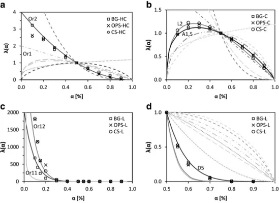
According to this, the most suitable decomposition reaction model for each biomass pseudo-component was determined using the generalized master plots procedure, which is valid only for single-stage process analysis, where there is no de-pendence of Eaon α [18]. Experimental data were normalized

to α = 0.5 using Eq.6, and compared with theoretical master plots in Fig.1. Activation energy in Eq.6is the mean value calculated for each pseudo-component using the mentioned three isoconversional methods.

Figure 5a shows that for the three biomasses, pseudo-hemicellulose matches closely the theoretical plot of a second-order kinetic model (Or2), except at low conversion (α < 0.2), where the decomposition model of OPS and CS

Table 6 Mean activation energy values of OPS, CS, and BG pseudo-components, calculated using Friedman, KAS, and FWO model-free methods Apparent activation energy: Ea(kJ/mol), σ (kJ/mol)

Pseudo-hemicellulose Pseudo-cellulose Pseudo-lignin

Friedman KAS FWO Friedman KAS FWO Friedman KAS FWO BG 167.8 σ = 1.1 163.2 σ = 12.2 164.2 σ = 11.9 191.0 σ = 7.1 211.3 σ = 6.2 210.7 σ = 5.8 198.4 σ = 5.8 221.2 σ = 7.0 221.0 σ = 7.5 CS 189.9 σ = 10.0 175.9 σ = 8.2 175.9 σ = 8.0 222.5 σ = 6.8 219.8 σ = 6.5 218.5 σ = 6.3 235.8 σ = 4.4 228.3 σ = 3.9 226.9 σ = 4.8 OPS 217.0 σ = 10.5 195.8 σ = 11.4 194.6 σ = 10.7 234.1 σ = 7.8 240.0 σ = 3.3 240.9 σ = 3.2 237.3 σ = 7.6 249.5 σ = 5.8 248.2 σ = 6.5 1.4 1.2 1.0 0.8 0.6 0.4 0.2 0.0 100 200 300 400 500 600 700

dα

/dT

[1

/°

C]

Temperature [°C]

a

dα

/dT

[1/°

C]

Temperature [°C]

b

dα

/dT

[1

/°

C]

Temperature [°C]

c

Fig. 3 Comparison between experimental curves and Fraser-Suzuki deconvolution results of a BG at 10 °C/min, b CS at 10 °C/min, and c OPS at 10 °C/min. HC pseudo-hemicellulose, C pseudo-cellulose, P-L pseudo-lignin

pseudo-hemicellulose is between first order and second order. For its part, BG is close to a second-order kinetic model in all the decomposition range. These differences at low conversion could be possibly due to interactions between the hemicellu-lose and the other biomass components. Similar approaches to other types of lignocellulosic biomasses have concluded that pseudo-hemicellulose decomposition follows an order-based kinetic model with n between 1.5 and 4 [50].

Master plots in Fig.5b show that pseudo-cellulose decompo-sition is in agreement with a random scission or an Avrami-Erofeev kinetic model, for the three studied biomasses. Notably, BG pseudo-cellulose matches better with an A1.5 Avrami-Erofeev nucleation and growth model, while OPS and CS pseudo-cellulose are closer to a L2 random scission model. Theoretical master plots of both models are close and are related to narrow reaction profiles, as seen in Fig. 4, where pseudo-cellulose decomposition range is narrower compared with

pseudo-hemicellulose and pseudo-lignin. In general, Avrami-Erofeev models assume that reaction or decomposition is due to the appearance of random nuclei and their subsequent growth, while random scission is related to the arbitrary break of poly-mer chains into smaller segments [30,51]. As the shape of both models is very close, it is not easy to consistently distinguish between them, in spite of the differences in their theoretical background. According to this, from a mathematical point of view, both of these models could describe the pseudo-cellulose decomposition mechanism. Similar studies reported for cellu-lose in the literature have concluded that both Avrami-Erofeev and random scission models could be suitable for the description of the cellulose thermal decomposition [22,36,52].

Finally, as seen in Fig.5c, pseudo-lignin decomposition does not match with any known theoretical kinetic model. Due to the complexity of the lignin structure and its inter-actions with the other biomass components [44,48,49], it

is not easy to fully understand its decomposition mecha-nism. As the cementing agent of biomass, lignin could interact with hemicellulose and cellulose in different ways according to the biomass structure and operating condi-tions. Moreover, lignin decomposes in a wide range of temperature and with low decomposition rate, making it difficult to completely model its corresponding reaction mechanism. At low conversion (α < 0.5), pseudo-lignin decomposition could be modeled by an order reaction mechanism, with n between 11 and 12 (Fig. 5c). From α = 0.5 to α = 0.9, decomposition is near a three-dimensional diffusion mechanism. Particularly, a D5 mod-el (Zhuravlev, Lesokin, Tempmod-elman), as presented in Fig. 5d. Other reported studies have described pseudo-lignin decomposition with a third-order reaction model [24], or even a high-order model with n > 12 [22]. The

proposed models, however, do not fit completely the pseudo-lignin the decomposition, due to its complexity.

With the knowledge of the most suitable reaction model for each pseudo-component, pre-exponential fac-tor A values were calculated. Taking into account that the difference between the apparent activation energy calculated with the Friedman, KAS, and FWO methods is not significant, E_a of each biomass pseudo-component was defined as the mean value of the activation energy estimated with the three methods. Furthermore, the Friedman method was chosen for the evaluation of the pre-exponential factor.

The dependence of ln (A) on α, presented in Fig. 6, is similar to that of the activation energy, remaining almost con-stant during all the conversion range (0.1 < α < 0.9). The relative standard deviation was in all cases inferior to 8% with

Fig. 6 Pseudo-component dependence of Ln (A) on the reaction extent. a Pseudo-hemicellulose. b Pseudo-cellulose. c Pseudo-lignin Fig. 5 Comparison between the

experimental and theoretical master plots for the three biomass pseudo-components. a hemicellulose. b Pseudo-cellulose. c Pseudo-lignin. d Pseudo-lignin (0.5 < α < 1.0)

values of even 2%. Accordingly, the mean values of Eaand A

for the three biomasses are summarized in Table7.

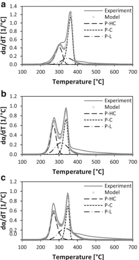
These kinetic parameters were validated and used to repro-duce the experimental decomposition curves of each biomass from 2 to 20 °C/min. For the three studied materials, a good agreement was found between the experimental data and the computed decomposition behavior, with fitting errors below 10% in all cases. Figure7shows the modeled decomposition rate of the three biomasses and pseudo-components at a heating rate of 10 °C/min.

It is possible to observe from this figure that there is a gap between experimental and modeled data at temperatures

above 400 °C, for the three biomasses. Comparing these re-sults with Fraser-Suzuki fitting presented in Fig.4, it can be noticed that the behavior of modeled pseudo-hemicellulose and pseudo-cellulose is in good agreement with the deconvolution patterns initially proposed. As a result, a good agreement is also obtained between modeled and experimen-tal decomposition at temperatures below 400 °C. In contrast, it is clear that the main differences observed are related to pseu-do-lignin. This is principally due to the complexity of model-ing the pseudo-lignin decomposition behavior in the investi-gated temperature range. In spite of this, the fitting error below 10% for the three materials showed that the calculated kinetic parameters using model-free isoconversional methods are suitable for the description of the biomass thermal decomposition.

Conclusion

In this study, the thermal decomposition of three lignocellu-losic biomasses with different macromolecular composition but nearly the same H/C and O/C fraction was investigated. Bamboo guadua (BG), coconut shells (CS), and oil palm shells (OPS) were used.

In general, the approach presented in this paper using a PRM using Fraser-Suzuki deconvolution and model-free isoconversional methods proved to be suitable to determine the pyrolysis kinetic parameters of biomasses with H/C and O/ C near 1.5 and 0.8. Despite the differences in the hemicellu-lose, celluhemicellu-lose, and lignin fraction of biomasses, any of the presented isoconversional methods can be used to calculate and predict the pseudo-component activation energy and pre-exponential factor, and to estimate their decomposition mech-anism. This information could constitute a valuable tool for reactor design and for the development and scale-up of pyrol-ysis and gasification processes using tropical lignocellulosic agrowastes as a feedstock.

The apparent activation energy of biomass pseudo-components followed the same behavior for the three studied materials: pseudo-hemicellulose Ea < pseudo-cellulose

Ea< pseudo-lignin Ea. Regarding the decomposition

mecha-nism, pseudo-hemicellulose and pseudo-cellulose were well described by a second-order model and a random-scission or an A1.5 Avrami-Erofeev model, respectively. For its part, pseudo-lignin decomposition did not completely match with

1.4 1.2 1.0 0.8 0.6 0.4 0.2 0.0 100 200 300 400 500 600 700 dα /dT [1 /° C] Temperature [°C]

a

b

c

Fig. 7 Comparison between experimental and modeled decomposition curves of a BG at 10 °C/min, b CS at 10 °C/min, and c OPS at 10 °C/min. Modeled curves generated using the calculated Ea and A values presented in Table7for biomasses and their pseudo-components

Table 7 Average Eaand A values

calculated for BG, CS, and OPS pseudo-components

Pseudo-hemicellulose Pseudo-cellulose Pseudo-lignin

Biomass Ea(kJ/mol) A (s−1) Ea(kJ/mol) A (s−1) Ea(kJ/mol) A (s−1)

BG 165.1 2.62E+14 204.3 2.30E+16 214.5 1.02E+18 CS 180.6 5.83E+16 220.3 2.30E+18 230.3 1.47E+21 OPS 202.4 6.33E+18 238.1 3.50E+19 245.0 8.83E+21

any known theoretical model, and was described by a combi-nation of a high-order model with n between 11 and 12 and a third dimension diffusion model. Lignin behavior was possi-bly due to the complexity of its structure and to the interac-tions with the other biomass components.

Differences between the calculated kinetic parameters of BG, CS, and OPS showed that biomass structure and molec-ular composition play a role in the biomass decomposition characteristics. Considering the nature of lignin, it could have an impact in the required energy to decompose hemicellulose and cellulose. The apparent activation energy for the three biomass pseudo-components followed the order BG Ea< CS

Ea< OPS Ea, with OPS and BG being the highest lignin and

lowest lignin content biomasses analyzed in this study, respec-tively. For the three studied materials, the model fitting error below 10% showed that the calculated kinetic parameters using model-free isoconversional methods are suitable for the description and prediction of the biomass thermal decomposition.

Acknowledgements The authors gratefully acknowledge COLCIENCIAS, for the doctoral scholarship awarded in the frame of the Colombian National Program for Doctoral Formation 647-2014.

References

1. Ullah K, Kumar Sharma V, Dhingra S et al (2015) Assessing the lignocellulosic biomass resources potential in developing countries: a critical review. Renew Sust Energ Rev 51:682–698. doi:10.1016/ j.rser.2015.06.044

2. Escalante H, Orduz J, Zapata HJ, et al (2010) Potencial energético de la biomasa residual. In: Ministerio de Minas y Energia -Republica de Colombia (ed) Atlas del Potencial Energético Biomasa Residual en Colomb. pp 155–172

3. García NJ a, EE YA (2010) Generación y uso de biomasa en plantas de beneficio de palma de aceite en Colombia—Power generation and use of biomass at palm oil mills in Colombia. Rev Palmas 31: 41–48

4. Food and Agriculture Organisation of the United Nations (2014) FAO statistical yearbook 2014: Latin America and the Caribbean. Santiago de Chile

5. Fryda L, Daza C, Pels J et al (2014) Lab-scale co-firing of virgin and torrefied bamboo species Guadua angustifolia Kunth as a fuel substitute in coal fired power plants. Biomass Bioenergy 65:28–41. doi:10.1016/j.biombioe.2014.03.044

6. Londoño X, Camayo GC, Riaño N, López Y (2002) Characterization of the anatomy of Guadua angustifolia (Poaceae: Bambusoideae) culms. Bamboo Sci Cult 16:18–31 7. Kuo P-C, Wu W, Chen W-H (2014) Gasification performances of

raw and torrefied biomass in a downdraft fixed bed gasifier using thermodynamic analysis. Fuel 117:1231–1241. doi:10.1016/j.fuel. 2013.07.125

8. Wongsiriamnuay T, Kannang N, Tippayawong N (2013) Effect of operating conditions on catalytic gasification of bamboo in a fluid-ized bed. Int J Chem Eng. doi:10.1155/2013/297941

9. Chen D, Liu D, Zhang H et al (2015) Bamboo pyrolysis using TG– FTIR and a lab-scale reactor: analysis of pyrolysis behavior,

product properties, and carbon and energy yields. Fuel 148:79– 86. doi:10.1016/j.fuel.2015.01.092

10. Forero Núñez CA, Cediel A, Hernández LC, et al (2012) Oil palm empty bunch fruits and coconut shells gasification using a lab-scale downdraft fixed bed gasifier at Universidad Nacional de Colombia. In: 20th Eur. Conf. Exhib. Milan, Italy, pp 1112–1114

11. Romero Millán LM, Cruz Domínguez MA, Sierra Vargas FE (2016) Efecto de la temperatura en el potencial de aprovechamiento energético de los productos de la pirólisis del cuesco de palma. Rev Tecnura 20:89–99. doi:10.14483/udistrital.jour.tecnura.2016.2.a06

12. Basu P (2013) Pyrolysis. In: Biomass gasification, pyrolysis and torrefaction, Second Edi. Elsevier Inc., London, pp 147–176 13. David E, Kopac J (2014) Activated carbons derived from residual

biomass pyrolysis and their CO2 adsorption capacity. J Anal Appl Pyrolysis 110:322–332. doi:10.1016/j.jaap.2014.09.021

14. Ye L, Zhang J, Zhao J et al (2015) Properties of biochar obtained from pyrolysis of bamboo shoot shell. J Anal Appl Pyrolysis 114: 172–178. doi:10.1016/j.jaap.2015.05.016

15. Abnisa F, Arami-Niya A, Wan Daud WMA et al (2013) Utilization of oil palm tree residues to produce bio-oil and bio-char via pyrol-ysis. Energy Convers Manag 76:1073–1082. doi:10.1016/j. enconman.2013.08.038

16. White JE, Catallo WJ, Legendre BL (2011) Biomass pyrolysis ki-netics: a comparative critical review with relevant agricultural res-idue case studies. J Anal Appl Pyrolysis 91:1–33. doi:10.1016/j. jaap.2011.01.004

17. Vyazovkin S, Wight CA (1999) Model-free and model-fitting ap-proaches to kinetic analysis of isothermal and nonisothermal data. Thermochim Acta 340:53–68. doi: 10.1016/S0040-6031(99)00253-1

18. Vyazovkin S, Burnham AK, Criado JM et al (2011) ICTAC kinetics committee recommendations for performing kinetic computations on thermal analysis data. Thermochim Acta 520:1–19. doi:10.1016/ j.tca.2011.03.034

19. Huang X, Cao J-P, Zhao X-Y et al (2016) Pyrolysis kinetics of soybean straw using thermogravimetric analysis. Fuel 169:93–98. doi:10.1016/j.fuel.2015.12.011

20. Ma Z, Chen D, Gu J et al (2015) Determination of pyrolysis char-acteristics and kinetics of palm kernel shell using TGA–FTIR and model-free integral methods. Energy Convers Manag 89:251–259. doi:10.1016/j.enconman.2014.09.074

21. Slopiecka K, Bartocci P, Fantozzi F (2012) Thermogravimetric analysis and kinetic study of poplar wood pyrolysis. Appl Energy 97:491–497. doi:10.1016/j.apenergy.2011.12.056

22. Wang X, Hu M, Hu W et al (2016) Thermogravimetric kinetic study of agricultural residue biomass pyrolysis based on combined kinet-ics. Bioresour Technol 219:510–520. doi:10.1016/j.biortech.2016. 07.136

23. Perejón A, Sánchez-Jiménez PE, Criado JM, Pérez-Maqueda LA (2011) Kinetic analysis of complex solid-state reactions. A new deconvolution procedure. J Phys Chem B 115:1780–1791. doi:10. 1021/jp110895z

24. Hu M, Chen Z, Wang S et al (2016) Thermogravimetric kinetics of lignocellulosic biomass slow pyrolysis using distributed activation energy model, Fraser–Suzuki deconvolution, and iso-conversional method. Energy Convers Manag 118:1–11. doi:10.1016/j. enconman.2016.03.058

25. Janković B (2015) Devolatilization kinetics of swine manure solid pyrolysis using deconvolution procedure. Determination of the bio-oil/liquid yields and char gasification. Fuel Process Technol 138:1– 13. doi:10.1016/j.fuproc.2015.04.027

26. Taghizadeh MT, Yeganeh N, Rezaei M (2014) Kinetic analysis of the complex process of poly(vinyl alcohol) pyrolysis using a new coupled peak deconvolution method. J Therm Anal Calorim 118: 1733–1746. doi:10.1007/s10973-014-4036-4

27. Cuéllar A, Muñoz I (2010) Fibra de guadua como refuerzo de matrices poliméricas - Bamboo fiber reinforcement for polymer matrix. DYNA 77:137–142. doi:10.15446/dyna

28. Mortley Q, Mellowes WA, Thomas S (1988) Activated carbons from materials of varying morphological structure. Themochim Acta 129:173–186. doi:10.1016/0040-6031(88)87334-9

29. García-Núñez JA, García-Pérez M, Das KC (2008) Determination of kinetic parameters of thermal degradation of palm oil mill by-products using thermogravimetric analysis and differential scanning calorimetry. Trans ASABE 51:547–557. doi:10.13031/2013.24354

30. Brown ME (1998) Handbook of thermal analysis and calorimetry. Volume 1. Principles and practice, First Edit. Elsevier

31. Anca-Couce A, Berger A, Zobel N (2014) How to determine con-sistent biomass pyrolysis kinetics in a parallel reaction scheme. Fuel 123:230–240. doi:10.1016/j.fuel.2014.01.014

32. Anca-Couce A, Zobel N, Berger A, Behrendt F (2012) Smouldering of pine wood: kinetics and reaction heats. Combust Flame 159:1708–1719. doi:10.1016/j.combustflame.2011.11.015

33. Svoboda R, Málek J (2013) Applicability of Fraser–Suzuki func-tion in kinetic analysis of complex crystallizafunc-tion processes. J Therm Anal Calorim 111:1045–1056. doi: 10.1007/s10973-012-2445-9

34. Rajeshwari P, Dey TK (2016) Advanced isoconversional and mas-ter plot analyses on non-isothermal degradation kinetics of AlN (nano)-reinforced HDPE composites. J Therm Anal Calorim 125: 369–386. doi:10.1007/s10973-016-5406-x

35. Gotor FJ, Criado JM, Malek J, Koga N (2000) Kinetic analysis of solid-state reactions: the universality of master plots for analyzing isothermal and nonisothermal experiments. J Phys Chem A:10777– 10782. doi:10.1021/jp0022205

36. Sánchez-Jiménez PE, Pérez-Maqueda LA, Perejón A, Criado JM (2013) Generalized master plots as a straightforward approach for determining the kinetic model: the case of cellulose pyrolysis. Thermochim Acta 552:54–59. doi:10.1016/j.tca.2012.11.003

37. Kan T, Strezov V, Evans TJ (2016) Lignocellulosic biomass pyrol-ysis: a review of product properties and effects of pyrolysis param-eters. Renew Sust Energ Rev 57:1126–1140. doi:10.1016/j.rser. 2015.12.185

38. Yang H, Yan R, Chen H et al (2007) Characteristics of hemicellu-lose, cellulose and lignin pyrolysis. Fuel 86:1781–1788. doi:10. 1016/j.fuel.2006.12.013

39. Liu Q, Zhong Z, Wang S, Luo Z (2011) Interactions of biomass components during pyrolysis: a TG-FTIR study. J Anal Appl Pyrolysis 90:213–218. doi:10.1016/j.jaap.2010.12.009

40. Mendu V, Harman-Ware AE, Crocker M et al (2011) Identification and thermochemical analysis of high-lignin feedstocks for biofuel

and biochemical production. Biotechnol Biofuels 4:43. doi:10. 1186/1754-6834-4-43

41. Collard F-X, Blin J (2014) A review on pyrolysis of biomass con-stituents: mechanisms and composition of the products obtained from the conversion of cellulose, hemicelluloses and lignin. Renew Sust Energ Rev 38:594–608. doi:10.1016/j.rser.2014.06. 013

42. Stefanidis SD, Kalogiannis KG, Iliopoulou EF et al (2014) A study of lignocellulosic biomass pyrolysis via the pyrolysis of cellulose, hemicellulose and lignin. J Anal Appl Pyrolysis 105:143–150. doi:

10.1016/j.jaap.2013.10.013

43. Jiang G, Nowakowski DJ, Bridgwater AV (2010) A systematic study of the kinetics of lignin pyrolysis. Thermochim Acta 498: 61–66. doi:10.1016/j.tca.2009.10.003

44. Caballero JA, Conesa JA, Font R, Marcilla A (1997) Pyrolysis kinetics of almond shells and olive stones considering their organic fractions. J Anal Appl Pyrolysis 42:159–175. doi: 10.1016/S0165-2370(97)00015-6

45. Chen Z, Hu M, Zhu X et al (2015) Characteristics and kinetic study on pyrolysis of five lignocellulosic biomass via thermogravimetric analysis. Bioresour Technol 192:441–450. doi:10.1016/j.biortech. 2015.05.062

46. Barneto AG, Carmona JA, Alfonso JEM, Serrano RS (2010) Simulation of the thermogravimetry analysis of three non-wood pulps. Bioresour Technol 101:3220–3229. doi:10.1016/j.biortech. 2009.12.034

47. Branca C, Albano A, Di Blasi C (2005) Critical evaluation of global mechanisms of wood devolatilization. Thermochim Acta 429:133– 141. doi:10.1016/j.tca.2005.02.030

48. Gani A, Naruse I (2007) Effect of cellulose and lignin content on pyrolysis and combustion characteristics for several types of bio-mass. Renew Energy 32:649–661. doi:10.1016/j.renene.2006.02. 017

49. Lv D, Xu M, Liu X et al (2010) Effect of cellulose, lignin, alkali and alkaline earth metallic species on biomass pyrolysis and gasifica-tion. Fuel Process Technol 91:903–909. doi:10.1016/j.fuproc.2009. 09.014

50. Hu S, Jess A, Xu M (2007) Kinetic study of Chinese biomass slow pyrolysis: comparison of different kinetic models. Fuel 86:2778– 2788. doi:10.1016/j.fuel.2007.02.031

51. Sanchez-Jimenez PE, Pérez-Maqueda LA, Perejon A, Criado JM (2010) Generalized kinetic master plots for the thermal degradation of polymers following a random scission mechanism. J Phys Chem A 114:7868–7876. doi:10.1021/jp103171h

52. Burnham AK, Zhou X, Broadbelt LJ Critical review of the global chemical kinetics of cellulose thermal decomposition. doi:10.1021/ acs.energyfuels.5b00350