An empirical comparison of V -fold penalisation and cross-validation for model selection in distribution-free regression
Texte intégral
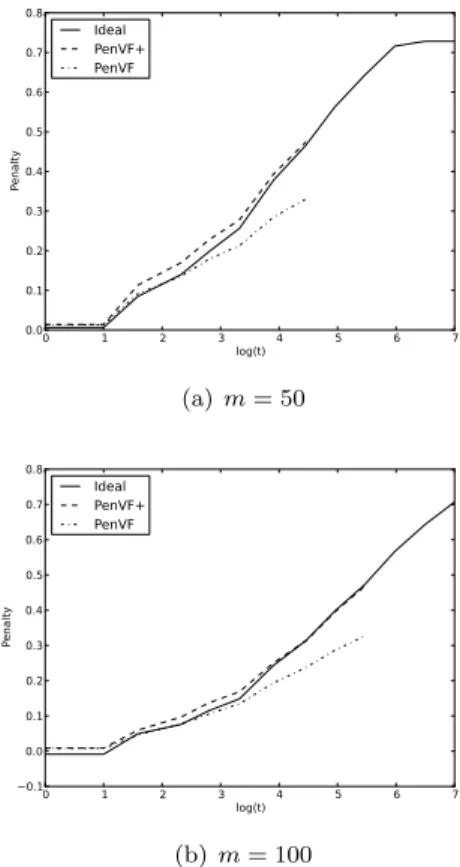
Figure
Documents relatifs
The initial condition is the following: at time zero, each site in x ∈ Z bears a random number of particles whose distribution is Poisson with parameter ρ > 0, the.. Key words
Domain disruption and mutation of the bZIP transcription factor, MAF, associated with cataract, ocular anterior segment dysgenesis and coloboma Robyn V.. Jamieson1,2,*, Rahat
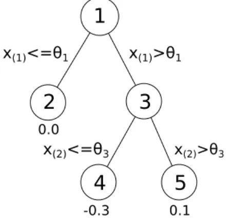
Like the unordered variable selection, the change-points detection problem is an illustration of such a framework since the number of models of dimension D is equals to ¡ D−1 n −1
We have presented analytical results on the existence of needle crystal solutions in the 2-D one-sided model of dendritic growth in the small and finite undercooling
In a general statistical framework, the model selection performance of MCCV, VFCV, LOO, LOO Bootstrap, and .632 bootstrap for se- lection among minimum contrast estimators was
This shows asymptotic optimality of the procedure and extends to the case of the selection of linear models endowed with a strongly localized basis structure, previous
Key words: V -fold cross-validation, V -fold penalization, model selection, non- parametric regression, heteroscedastic noise, random design, wavelets..
Keywords: Model Driven Engineering, Aspect Oriented Modeling, Model Composition Validation, Model Validation, Model Driven Engineering for Adaptive Systems.. 1
