Surface-Wave Images of Western Canada: Lithospheric Variations
1Across the Cordillera/Craton Boundary
23 4
T. Zaporozan, Department of Geological Sciences, University of Manitoba,
5
A.W. Frederiksen1, Department of Geological Sciences, University of Manitoba,
7
A. Bryksin, Department of Geological Sciences, University of Manitoba,
9
F. Darbyshire, Centre de recherche GEOTOP, Université du Québec à Montréal,
11
13 14
Manuscript for Canadian Journal of Earth Sciences, revised for resubmission. 15
1 Corresponding author. Full address: A.W. Frederiksen, Department of Geological Sciences, University of
Abstract
16
Two-station surface-wave analysis was used to measure Rayleigh-wave phase velocities 17
between 105 station pairs in western Canada, straddling the boundary between the tectonically 18
active Cordillera and the adjacent stable craton. Major variations in phase velocity are seen 19
across the boundary at periods from 15 to 200 s, periods primarily sensitive to upper-mantle 20
structure. Tomographic inversion of these phase velocities was used to generate phase-velocity 21
maps at these periods, indicating a sharp contrast between low-velocity Cordilleran upper mantle 22
and high-velocity cratonic lithosphere. Depth inversion along selected transects indicates that the 23
Cordillera/craton upper-mantle contact varies in dip along the deformation front, with cratonic 24
lithosphere of the Taltson province overthrusting Cordilleran asthenosphere in the northern 25
Cordillera, and Cordilleran asthenosphere overthrusting Wopmay lithosphere further south. 26
Localized high-velocity features at sub-lithospheric depths beneath the Cordillera are interpreted 27
as Farallon slab fragments, with the gap between these features indicating a slab window. A 28
high-velocity feature in the lower lithosphere of the Slave province may be related to Proterozic 29
or Archean subduction. 30
31
Keywords: Seismology, surface waves, tomography, Cordillera, craton
32 33 34
1. Introduction
35
The lithosphere beneath stable continental regions typically exhibits elevated seismic 36
velocities to depths of 200 km or more, which has been attributed to a combination of low 37
temperature and depleted composition (e.g. King 2005, Artemieva 2009, Aulbach 2012). By 38
contrast, young orogenic belts are underlain by low-velocity upper mantle, attributed to a 39
combination of high temperature, elevated volatile content, and a component of partial melt (see 40
e.g. Hyndman et al. 2009). In North America, these two lithospheric regimes exist in close 41
juxtaposition where the Phanerozoic Cordilleran Orogen abuts on Precambrian ancestral North 42
America (Figure 1). Previous tomographic studies of North America (van der Lee and Nolet 43
1997a, Frederiksen et al. 2001, Bedle and Van der Lee 2009, Schaeffer and Lebedev 2014) 44
image the Cordillera-craton transition as a major lithospheric velocity contrast, but questions 45
remain regarding the sharpness of the transition, its orientation in three dimensions, and its 46
relationship to crustal boundaries. We present a new study of the upper mantle beneath western 47
Canada, based on two-station surface-wave analysis, that brings new constraints to bear on these 48
questions. 49
East of the Cordillera, Western Canada is a Precambrian craton assemblage accreted in 50
the Proterozoic from Archean and younger blocks (Whitmeyer and Karlstrom 2007). The Slave, 51
Superior, Rae, Hearne, and Sask cratons are all of Archean age. These cratons assembled during 52
the Proterozoic via the Taltson, Wopmay, and Trans-Hudson orogens. Their western boundary 53
was a passive rifted margin in the Late Proterozoic (Gabrielse and Yorath 1991), onto which a 54
series of terranes were accreted, beginning with the Intermontane Superterrane in the Jurassic 55
(Clowes et al. 2005). This collision produced a fold-and-thrust belt extending to the current 56
Cordilleran deformation front. A later collision of the Insular Superterrane in the Cretaceous 57
extended the Cordillera westward to its present extent. 58
2. Data and analysis
59
The Geological Survey of Canada (GSC) operates the Canadian National Seismograph 60
Network (CNSN), which has been recording digital broadband data since the early 1990s (North 61
and Basham 1993). Further instrumentation was installed as part of the Portable Observatories 62
for Lithospheric Analysis and Research Investigating Seismicity (POLARIS) project (Eaton et al. 63
2005), the data from which is also archived by the GSC. We collected data from CNSN and 64
POLARIS stations in western and central Canada, corresponding to earthquakes of magnitude 65
greater than 6, at any distance from the receivers, whose propagation paths lay within 5° of the 66
paths between selected station pairs (Figure 2). These pairs were selected to give consistent 67
coverage of western Canada, and do not include all possible station pairs, particularly in western 68
British Columbia where stations are more closely spaced than is appropriate for the intended 69
resolution of this study. The downloaded data were inspected for Rayleigh-wave signal quality 70
before use. The station responses were removed by conversion to displacement before further 71
analysis; all stations used are broad-band, with all but two stations (ILKN and VGZ) having 72
significant velocity response (at least 10% of the peak value) to periods of 200 s or longer. A plot 73
of instrument responses is provided as supplemental material. 74
Two-station surface-wave analysis is a widely-used technique with a long history 75
(beginning with Sato 1955) in which the change in waveform between two receiving stations is 76
measured. Under the assumption that the waveform change is determined entirely by the 77
structure along the great-circle path connecting the station pair, the waveform change may be 78
used to isolate structure between the receiving instruments, even in aseismic regions. Thus, two-79
station analysis is appropriate for Canada, which has limited seismic activity away from the west 80
coast; previous studies have successfully applied this approach to the Canadian Arctic 81
(Darbyshire 2005), Hudson Bay (Darbyshire and Eaton 2010), the Superior Province (Darbyshire 82
et al. 2007), the southern Cordillera (Bao et al. 2014), and the northern Cordillera (McLellan et 83
al. 2018). 84
Two-station analysis is generally applied at large distances from the earthquake source. 85
Under these conditions, the different surface-wave modes are well separated and the fundamental 86
Rayleigh mode dominates vertical-component recordings. A single mode’s propagation may be 87
described by a dispersion curve showing the relationship between frequency and velocity; the 88
velocity considered may be either group velocity (velocity of energy transport, measured by 89
determining the travel time of the signal envelope peak) or phase velocity (velocity of the phase 90
of a single frequency, measured by determining the phase shift over a given distance). As the 91
group velocity dispersion curve may be determined from the phase velocity, but not vice versa, 92
the phase velocity contains more information (see e.g. Stein and Wysession 2003). 93
We measure phase-velocity dispersion curves using the cross-correlation technique of 94
Meier et al. (2004); an example is given in Figure 3. Two vertical-component recordings of the 95
same event, at stations that lie within 5° of a common great-circle path to the source, are cross-96
correlated. The phase of the cross-correlation corresponds to the phase difference between the 97
two traces, with an ambiguity of 2𝜋𝑛 radians, where n is an integer. For a cross-correlation phase 98
of Φ measured between two stations separated by a distance x at angular frequency ω, the phase 99 velocity will be 100 𝑐(𝜔) = 𝑥𝜔 𝜙 + 2𝜋𝑛 101
and therefore multiple velocities are compatible with the measurement, the possible solutions 102
being more closely spaced at higher frequencies. In practical use, the distance x is taken to be the 103
difference between the source-receiver distances for each station, to avoid biased measurements 104
for events not perfectly aligned with the two-station path. At sufficiently low frequency, there is 105
likely to be only one phase-velocity value that falls within a realistic range; thus, the approach of 106
Meier et al. (2004) is to begin at the longest period with significant coherent energy, and 107
continue the dispersion curve to higher frequencies while assuming that the curve is smooth (as 108
large jumps in phase velocity are unphysical). Multiple events were analysed for each station 109
pair, incorporating paths travelling in both possible directions, and the resulting set of dispersion 110
curves was averaged to obtain a single high-quality curve for each station pair. Two stages of 111
quality control were performed: on individual paths, events were included in the average only in 112
frequency bands that showed consistency with other events, and on the averaged curves, paths 113
were edited to exclude frequency bands with strong deviations (more than 5%) from the average 114 of all paths. 115 3. Results 116 3.1 Dispersion curves 117
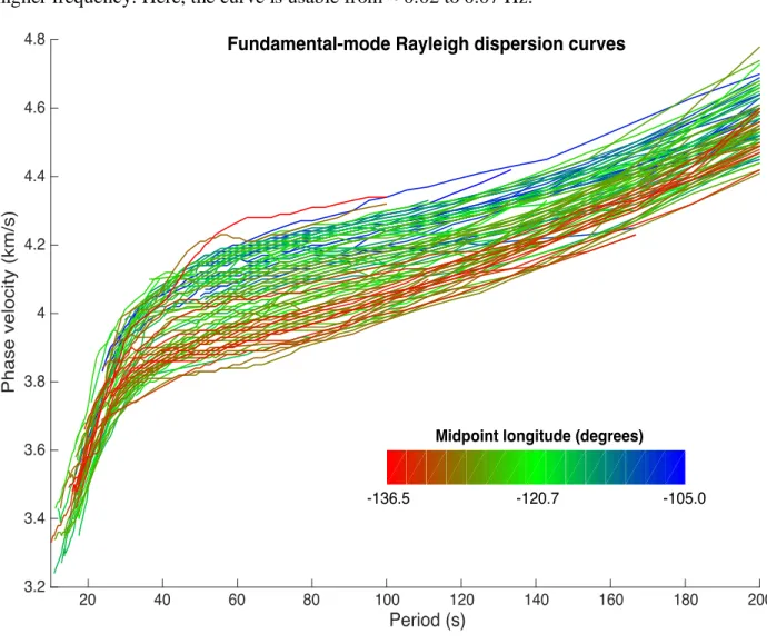
Figure 4 shows the complete set of dispersion curves obtained in this study, after quality 118
control was performed. A total of 105 curves was measured, at periods ranging from 16 to 333 s 119
depending on path length and data quality; generally speaking, longer periods were measurable 120
on longer paths and shorter periods on shorter paths. We do not, however, have high confidence 121
in the longest periods, which are sparsely sampled, and therefore only periods up to 200 s are 122
shown in the figure. The curves all show a velocity that increases with period, as would be 123
most sensitive to lithospheric depths, the path-to-path variation covers a range of ≈ 400 m/s. This 125
variation is systematic with path location, with eastern paths being faster and western paths being 126
slower. 127
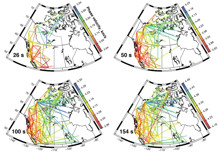
The spatial variation of phase velocities is more apparent in map view (Figure 5). At 128
relatively short periods (up to 50 s), low velocities are clearly restricted to the Cordillera, while 129
moderate to high velocities occur further east. At longer periods, more paths sampling both areas 130
are present; though there is still a trend of velocity increasing eastward, there are also a number 131
of crossing paths with distinctly different velocities. The true distribution of phase velocity 132
cannot be determined without tomographic inversion. 133
3.2 Tomographic resolution and maps
134
Under the assumption that two-station measurements represent averages along great-135
circle paths, the recovery of 2-D dispersion maps is a linear inverse problem (Montagner 1986). 136
We solved for a grid of phase velocities spaced 1° apart in latitude and 2° in longitude, with 137
smoothing and damping constraints; the correct regularization level was determined by the L-138
curve method (Parker 1994). Each period was solved for independently, yielding maps from 30 139
to 160 s at 10 s intervals. 140
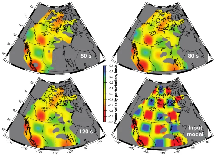
We performed lateral resolution tests using the path coverage for three relevant periods 141
(50, 80, and 120 s; Figure 6). For an input model consisting of 4° (latitude) by 8° (longitude) 142
blocks of alternating positive and negative 0.4 km/s velocity perturbations, we calculated average 143
velocities for each path, added errors comparable to the scatter in the real data, and inverted 144
using the same parameters as for the real data. The size of the blocks used reflects the feature 145
size we are able to recover: ~ 450 km over most of the map area. The results indicate that the 146
boundaries of features of this scale can be recovered accurately (within ~ 100 km) west of ~ 147
100°W and south of 70°N, albeit with significant underestimation of anomaly magnitudes, and 148
that resolution is best at moderate periods (60-100 s). Given that our regularization is smoothing-149
based, larger-scale features than this will be recovered more accurately. 150
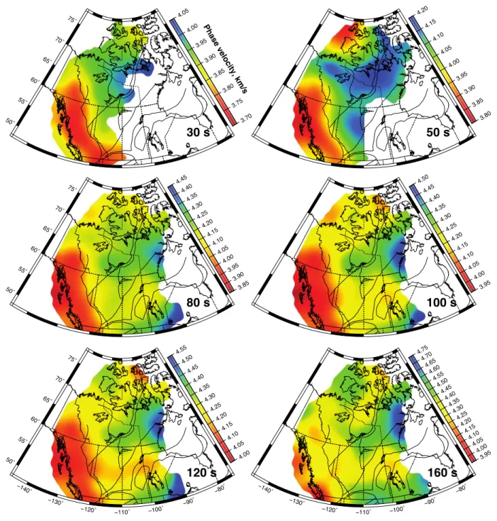
Final dispersion maps for the real data set are shown in Figure 7. The Cordillera is low-151
velocity at all periods, with the edge of the low-velocity region corresponding closely to the 152
Cordillera/craton boundary at periods of 80 s and less. At longer periods, the edge is more 153
complex, with low velocities extending some distance into the craton north of 52°N. The 154
Cordilleran low-velocity region is truncated north of 65°N at all periods; its southern and 155
western boundaries are not imaged by this study. 156
East of the Cordillera, phase velocities are moderate to high (e.g. > 4.2 km/s at 80 s 157
period). At short periods, resolution does not extend much east of 110°W due to a lack of high-158
frequency measurements along the longer paths in the eastern portion of the model. At periods of 159
80 s and higher, the highest phase velocities detected are at the eastern edge of the resolved 160
region, ca. 95°W. Localized high-velocity zones are detected beneath Great Slave Lake (at the 161
southern tip of the Slave Province) and along the southern edge of the model ca. 110°W. 162
3.3 Depth inversion and cross-sections
163
Rayleigh-wave period is often used as a depth proxy in surface-wave studies due to the 164
increase in depth sensitivity with period; however, as any given velocity measurement is 165
sensitive to a large range of depths, phase velocities must be inverted in order to constrain 166
seismic velocity as a function of depth. The depth sensitivity of Rayleigh-wave phase velocities 167
is model-dependent, requiring a nonlinear depth inversion. 168
We inverted for depth using the widely-used Computer Programs in Seismology package 169
(Herrmann 2013), using phase velocities extracted from the tomographic maps, at periods 170
ranging from 30 to 160 s at 10 s intervals, the range of periods at which we are most confident in 171
the map coverage. We used a starting model simplified from IASP91 (Kennett and Engdahl 172
1991), with fixed layer thicknesses ranging from 15 to 25 km (including a two-layer crust 35 km 173
thick; see Figure 8), and inverted for S velocity over 5 iterations, with P velocity determined 174
using a Poisson’s ratio fixed to match the base model values (which range from 0.20 to 0.29), 175
and density calculated from the P velocity. Smoothing regularization was used to compensate for 176
the non-uniqueness of the inversion and to encourage model simplicity. 177
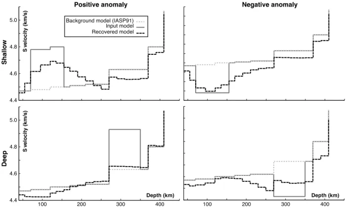
Synthetic tests of the depth inversion are shown in Figure 8. For each test, an input model 178
containing a large (300 m/s) perturbation from IASP91 was used to generate a dispersion curve, 179
using the same period sampling as the real data. The dispersion curve was then inverted (using 180
the same inversion parameters as the real data) to test recovery of the input. We find that low-181
velocity features are significantly smeared, but not missed; high-velocity features at relatively 182
shallow depth (above 150 km) are recovered, but produce a weaker low-velocity artefact below, 183
while deep high-velocity anomalies are poorly recovered. These effects are a consequence of the 184
non-linearity of surface-wave depth inversion, and will be less severe for weaker velocity 185
perturbations. 186
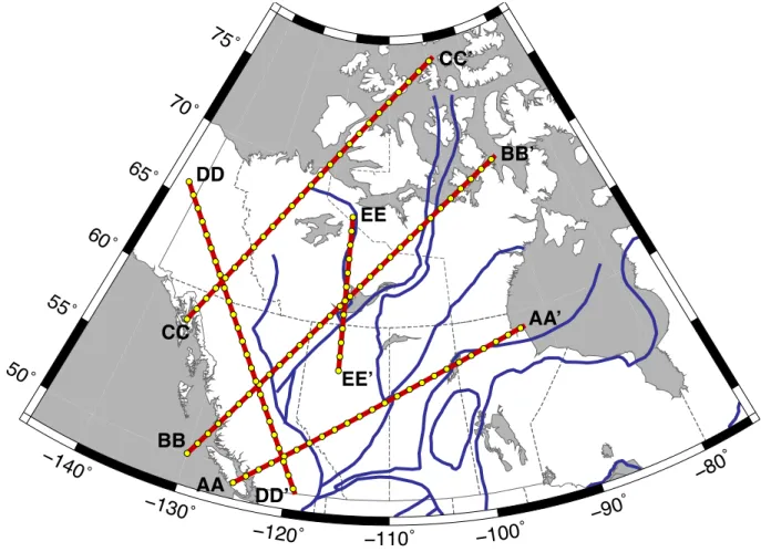
To generate cross-sections, we spatially interpolated phase velocities at 50 km intervals 187
from all dispersion maps, along five great-circle trajectories (Figure 9). The resulting dispersion 188
curves were then inverted to form 1-D S velocity models, as described above; the 1-D models 189
were concatenated to form a 2-D model along each transect. An example of this procedure is 190
given in Figure 10, in which the series of dispersion curves is presented as a pseudosection (top 191
panel) and inverted to obtain a velocity model (presented in both relative and absolute velocity 192
terms). It is worth noting that the lack of short-period sampling in some areas affects the 193
inversion; northeast of the 1100 km point along the transect, the shortest periods are not available 194
(due to longer two-station paths in this region) and the shallowest part of the model is not well 195
constrained. As a consequence, northeast of 1100 km, velocity anomalies appear weaker due to 196
upward smearing of structure into the poorly-sampled shallow depth range. We therefore expect 197
that mantle velocity anomalies will be somewhat underestimated in the more poorly-198
instrumented portions of the study area; this effect is most pronounced on the AA-AA’ section 199
shown in Figure 10. 200
Transects were selected to examine the Cordillera-craton transition along three near 201
boundary-perpendicular sections (AA-AA’, BB-BB’ and CC-CC’), along-strike variation within 202
the Cordilleran low-velocity anomaly (DD-DD’), and a high-velocity feature detected near Great 203
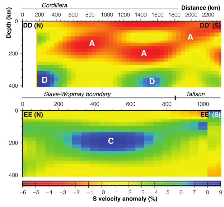
Slave Lake in the dispersion maps (EE-EE’). The Cordillera is underlain by a low-velocity 204
feature (marked as A on the cross-sections; Figures 11 and 12) averaging 2-4% below IASP91 205
velocity down to ~250 km depth. The adjacent cratonic lithosphere (B) is underlain by high-206
velocity lithosphere (5-8% above IASP91) down to 200-250 km depth; the contact between these 207
two anomalies is quite sharp (~ 8-10% over 200-300 lateral km at lithospheric depths), lies 208
directly beneath the crustal contact, and is not vertical. In the northern two cross-sections (CC-209
CC’ and BB-BB’; Figure 11) the contact dips 10-20° to the northeast, with cratonic lithosphere 210
overlying asthenospheric material associated with the Cordillera; by contrast, the southernmost 211
section (AA-AA’) shows a dip of ~ 30° in the opposite direction. The depth extent of Cordilleran 212
low velocities varies somewhat along strike, shallowing to ~ 150 km depth beneath southern 213
British Columbia (DD-DD’; Figure 12). Our synthetic tests showed that high velocities at 214
lithospheric depths can produce low-velocity artefacts below; however, the artefacts are 215
significantly weaker than the high-velocity anomalies they underlie, which is not the case where 216
feature A underlies feature B. 217
A localized high-velocity zone (feature C) centred on Great Slave Lake (62°N, 115°W) is 218
visible on longer-period dispersion maps (Figure 7). The two cross-sections that intersect this 219
zone (BB-BB’ and EE-EE’; Figures 11 and 12) show a high-velocity feature from ≈ 125-275 km, 220
extending somewhat deeper than is typical for cratonic lithosphere in North America (200-250 221
km; Eaton et al. 2009, Yuan et al. 2014). Even deeper high-velocity features (labelled D) are 222
seen in patches beneath the Cordillera and adjacent areas. 223
4. Discussion
224
The Cordilleran mantle velocities we have measured are very low – for instance, at 400 225
km along the BB-BB’ transect, the lowest mantle S velocity attained is 4.25 km/s from 155-170 226
km depth. Though a very low value for this depth (IASP91 reaches 4.51 km/s at 160 km), it is 227
consistent with the models of Van der Lee and Frederiksen (2005) and Schaeffer and Lebedev 228
(2014), which have comparable velocities in the same location. Based on the velocity-229
temperature calculations of Hyndman et al. (2009), this low velocity would correspond to a 230
temperature of ~ 1200-1250°C, which is in accordance with previous studies, implying 231
asthenospheric material underlying a weak, thin lithosphere and raising the possibility of small-232
scale convection in the Cordilleran upper mantle (Hyndman 2010). 233
Though our measurements of Cordilleran upper-mantle velocity primarily confirm earlier 234
studies, this study provides novel high-resolution constraints on a significant portion of the 235
Cordillera/craton boundary. Our cross-sections show that the mantle boundary is not vertical 236
(Figure 11), with some high-velocity material extending west of the Cordilleran deformation 237
front in the crust. This may help to explain why some models place the boundary west of the 238
front (see e.g. Frederiksen et al. 2001, McLellan et al. 2018). 239
Our most remarkable observation at the Cordillera/craton boundary is the change in dip 240
direction from northeastern (cratonic material overthrusting Cordilleran asthenosphere) on the 241
northern and central cross-sections (CC-CC’ and BB-BB’, Figure 11) to southwestern 242
(Cordilleran asthenosphere overthrusting cratonic lithosphere) in the southernmost cross-section. 243
This change, which was also detected in a recent North American model (Schaeffer et al. 2017), 244
is seen in previous smaller-scale models. Surface and body-wave models of the southern 245
Cordillera (Bao et al. 2014, Chen et al. 2017) show a steeply westward-dipping or vertical 246
boundary, while models of the northern Cordillera show northeast dips (Cook and Erdmer 2005, 247
Mercier et al. 2009). Models of the United States are not directly comparable due to the 248
influence of the Yellowstone hotspot. 249
A possible explanation for the difference in dip direction at the lithospheric contact may 250
be that the northern two cross-sections sample the Wopmay orogen, while the southernmost 251
cross-section intersects the Taltson. Though both of these orogens were assembled through 252
eastward-dipping subduction (McDonough et al. 2000, Davis et al. 2015), their western edges 253
consist of different terranes (the Hottah for the Wopmay and the Buffalo Head for the Taltson). 254
These terranes have different origins, and it is possible that their associated lithospheres are 255
rheologically distinct. Edge-driven convection has been proposed for the southern Cordillera 256
(Hardebol et al. 2012, Bao et al. 2014); modelling results indicate that mantle viscosity is an 257
important control on the behaviour of the Cordillera/craton transition. It is thus plausible that a 258
rheological difference between cratonic lithosphere of different affinity is affecting the shape of 259
the mantle boundary, but further modelling is needed to support this. 260
Localized high-velocity features at sub-lithospheric depths (feature D; Figures 11 and 12) 261
are found at various points beneath the Cordillera and craton. High velocities at these and greater 262
depths appear in a number of tomographic models (see e.g. van der Lee and Nolet 1997b, Ren et 263
al. 2007) and are commonly attributed to remnants of the subducted Farallon or Kula slab. The 264
lateral resolution of our model does not permit an interpretation of the lateral extent of these 265
features east of the Cordillera (as shown by the longest-period resolution test in Figure 6). 266
However, as our path density is highest within the Cordillera itself, the discontinuous nature of 267
feature D in section DD-DD’ is probably a real feature, though ~ 350 km depth is at the limit of 268
resolution for fundamental-mode Rayleigh waves. 269
Gaps in subducting slabs, resulting from processes such as ridge/trench contact, are 270
known in the literature as slab windows. Slab windows have been proposed to exist north and 271
south of the Juan de Fuca slab (Thorkelson and Taylor 1989); the southern window is seen in 272
northern California (Hawley et al., 2016), while an additional slab gap is visible as a low-273
velocity feature beneath Oregon (Tian and Zhao 2012). We interpret feature D as slab remnants 274
interrupted by a northern Cordilleran slab window, and therefore that the slab is absent from 400-275
1200 km along the DD-DD’ cross-section. This range corresponds well with lateral velocity 276
contrasts at ≈ 50°N and 60°N seen in the teleseismic P velocity model of Mercier et al. (2009). 277
The high-velocity feature labelled C in sections BB-BB’ and EE-EE’ cannot be attributed 278
to recent subduction. Its depth of 150-250 km beneath the stable craton places it at the base of 279
the lithosphere; its velocity of up to 10% over IASP91 is remarkable, indicating that it is fast 280
even relative to the generally high-velocity surrounding cratonic lithosphere. A high-velocity 281
feature beneath the Slave craton was previously found in this depth range using array analysis of 282
surface waves (Chen et al. 2007), while strongly-layered lithosphere is visible in receiver 283
functions (Bostock 1998). LITHOPROBE reflection data across the Slave craton’s eastern boundary 284
show dipping reflectors attributed to Proterozoic and Archean subduction (Cook et al. 1999) 285
which, when extrapolated eastward, correspond with receiver-function arrivals bracketing the 286
depth of feature C. We therefore propose that feature C preserves these subduction remnants in 287
the lower portion of the Slave lithosphere. 288
5. Conclusions
289
Through two-station analysis of surface-wave records, we have mapped Rayleigh phase 290
velocity across western Canada. The most salient feature of our dispersion maps is the sharp 291
contrast between low-velocity Cordilleran upper mantle and high-velocity cratonic lithosphere. 292
By extracting dispersion curves from the tomographic maps and inverting for S velocity 293
structure, we have generated cross-sections examining the Cordillera/craton mantle boundary 294
and surrounding region; these cross-sections show a change in dip of the mantle contact from 295
northeast in the northern Cordillera to southwest in the southern Cordillera, which may reflect 296
differences in rheology between the Wopmay and Taltson shield provinces. Isolated high-297
velocity features seen beneath the Cordilleran upper mantle may represent Farallon slab 298
fragments, separated by a gap resulting from a Cordilleran slab window. A high-velocity feature 299
at the base of the Slave Province lithosphere correlates with a previously interpreted Proterozoic 300
subduction feature. 301
The main limitation on these results is the lack of resolution east of the Cordillera due to 302
a limited station network. New instruments currently deployed in the Northern Cordillera (Ma 303
and Audet 2017) will allow improvement of these images in the future, as will incorporation of 304
instrumentation in the United States. 305
Acknowledgements
306
Funding for this research was provided by NSERC, the Geological Survey of Canada, 307
and de Beers Canada. Pascal Audet and Ian Ferguson provided essential feedback on the M.Sc. 308
thesis from which this paper is derived; thanks also to Andrew Schaeffer for helpful discussion. 309
Thanks to Derek Schutt and an anonymous reviewer for reviews that significantly improved this 310
manuscript. 311
References
313
Artemieva, I.M. 2009. The continental lithosphere: Reconciling thermal, seismic, and petrologic 314
data. Lithos 109(1-2): 23–46. doi:10.1016/j.lithos.2008.09.015. 315
Aulbach, S. 2012. Craton nucleation and formation of thick lithospheric roots. Lithos 149(C): 316
16–30. Elsevier B.V. doi:10.1016/j.lithos.2012.02.011. 317
Bao, X., Eaton, D.W., and Guest, B. 2014. Plateau uplift in western Canada caused by 318
lithospheric delamination along a craton edge. Nature Geoscience 7(11): 830–833. 319
doi:10.1038/ngeo2270. 320
Bedle, H., and Van Der Lee, S. 2009. S velocity variations beneath North America. J Geophys 321
Res-Sol Ea 114: –. doi:10.1029/2008JB005949. 322
Bostock, M.G. 1998. Mantle stratigraphy and evolution of the Slave province. J. Geophys. Res 323
103: 21183–21200.
324
Chen, C.-W., Rondenay, S., Weeraratne, D.S., and Snyder, D.B. 2007. New constraints on the 325
upper mantle structure of the Slave craton from Rayleigh wave inversion. Geophys Res Lett 326
34: –. doi:10.1029/2007GL029535.
327
Chen, Y., Gu, Y.J., and Hung, S.-H. 2017. Finite-frequency P-wave tomography of the Western 328
Canada Sedimentary Basin: Implications for the lithospheric evolution in Western Laurentia. 329
Tectonophysics 698(C): 79–90. Elsevier B.V. doi:10.1016/j.tecto.2017.01.006. 330
Clowes, R., Hammer, P.T., Fernández-Viejo, G., and Welford, J. 2005. Lithospheric structure in 331
northwestern Canada from Lithoprobe seismic refraction and related studies: a synthesis. 332
Can J Earth Sci 42(6): 1277–1294. 333
Cook, F.A., and Erdmer, P. 2005. An 1800 km cross section of the lithosphere through the 334
northwestern North American plate: lessons from 4.0 billion years of Earth's history. Can J 335
Earth Sci 42: 1295–1311. doi:10.1139/e04-106. 336
Cook, F.A., Velden, A.J., Hall, K.W., and Roberts, B.J. 1999. Frozen subduction in Canada's 337
Northwest Territories: Lithoprobe deep lithospheric reflection profiling of the western 338
Canadian Shield. Tectonics 18(1): 1–24. doi:10.1029/1998TC900016. 339
Darbyshire, F.A. 2005. Upper mantle structure of Arctic Canada from Rayleigh wave dispersion. 340
Tectonophysics 405(1-4): 1–23. doi:10.1016/j.tecto.2005.02.013. 341
Darbyshire, F.A., and Eaton, D.W. 2010. The lithospheric root beneath Hudson Bay, Canada 342
from Rayleigh wave dispersion No clear seismological distinction between Archean and 343
Proterozoic mantle. Lithos 120: 144–159. doi:10.1016/j.lithos.2010.04.010. 344
Darbyshire, F.A., Eaton, D.W., Frederiksen, A., and Ertolahti, L. 2007. New insights into the 345
lithosphere beneath the Superior Province from Rayleigh wave dispersion and receiver 346
function analysis. Geophys J Int 169: 1043–1068. doi:10.1111/j.1365-246X.2006.03259.x. 347
Davis, W.J., Ootes, L., Newton, L., Jackson, V., and Stern, R.A. 2015. Characterization of the 348
Paleoproterozoic Hottah terrane, Wopmay Orogen using multi-isotopic (U-Pb, Hf and O) 349
detrital zircon analyses: An evaluation of linkages to northwest Laurentian Paleoproterozoic 350
domains. Precambrian Research 269: 296–310. Elsevier B.V. 351
doi:10.1016/j.precamres.2015.08.012. 352
Eaton, D.W., Adams, J., Asudeh, I., Atkinson, G.M., Bostock, M.G., Cassidy, J.F., Ferguson, 353
I.J., Samson, C., Snyder, D.B., Tiampo, K.F., and Unsworth, M.J. 2005. Investigating 354
Canada's lithosphere and earthquake hazards with portable arrays. Eos 86(17): 169–171. 355
doi:10.1029/2005EO170001/full. 356
Eaton, D.W., Darbyshire, F.A., Evans, R.L., Grütter, H., Jones, A.G., and Yuan, X. 2009. The 357
elusive lithosphere–asthenosphere boundary (LAB) beneath cratons. Lithos 109(1-2): 1–22. 358
doi:10.1016/j.lithos.2008.05.009. 359
Frederiksen, A., Bostock, M.G., and Cassidy, J.F. 2001. S-wave velocity structure of the 360
Canadian upper mantle. 124: 175–191. 361
Gabrielse, H., and Yorath, C.J. 1991. Tectonic Synthesis. In Geology of the Cordilleran Orogen 362
in Canada. Edited by H. Gabrielse and C.J. Yorath. Accents Publications Service. pp. 677– 363
705. 364
Hardebol, N.J., Pysklywec, R.N., and Stephenson, R. 2012. Small‐scale convection at a 365
continental back‐arc to craton transition: Application to the southern Canadian Cordillera. 366
Journal of Geophysical Research: Solid Earth (1978–2012) 117(B1). 367
doi:10.1029/2011JB008431. 368
Hawley, W.B., Allen, R.M., and Richards, M.A. 2016. Tomography reveals buoyant 369
asthenosphere accumulating beneath the Juan de Fuca plate. Science 353(6306): 1406–1408. 370
American Association for the Advancement of Science. doi:10.1126/science.aad8104. 371
Herrmann, R.B. 2013. Computer Programs in Seismology: An Evolving Tool for Instruction and 372
Research. Seismological Research Letters 84(6): 1081–1088. GeoScienceWorld. 373
doi:10.1785/0220110096. 374
Hyndman, R. 2010. The consequences of Canadian Cordillera thermal regime in recent tectonics 375
and elevation: a review. Can J Earth Sci 47(5): 621–632. 376
Hyndman, R.D., Currie, C.A., Mazzotti, S., and Frederiksen, A. 2009. Temperature control of 377
continental lithosphere elastic thickness, Te vs Vs. Earth and Planetary Science Letters 277: 378
539–548. doi:10.1016/j.epsl.2008.11.023. 379
Kennett, B.L.N., and Engdahl, E.R. 1991. Traveltimes for global earthquake location and phase 380
identification. Geophysical Journal of the Royal Astronomical Society 105(2): 429–465. 381
Blackwell Publishing Ltd. doi:10.1111/j.1365-246X.1991.tb06724.x. 382
King, S.D. 2005. Archean cratons and mantle dynamics. Earth and Planetary Science Letters 383
234(1-2): 1–14. doi:10.1016/j.epsl.2005.03.007.
384
Ma, S., and Audet, P. 2017. Seismic velocity model of the crust in the northern Canadian 385
Cordillera from Rayleigh wave dispersion data. 54(2): 163–172. doi:10.1139/cjes-2016-386
0115. 387
McDonough, M.R., McNicoll, V.J., Schetselaar, E.M., and Grover, T.W. 2000. 388
Geochronological and kinematic constraints on crustal shortening and escape in a two-sided 389
oblique-slip collisional and magmatic orogen, Paleoproterozoic Taltson magmatic zone, 390
northeastern Alberta. Can J Earth Sci 37: 1549–1573. 391
McLellan, M., Schaeffer, A.J., and Audet, P. 2018. Structure and fabric of the crust and 392
uppermost mantle in the northern Canadian Cordillera from Rayleigh-wave tomography. 393
Tectonophysics 724-725: 28–41. Elsevier. doi:10.1016/j.tecto.2018.01.011. 394
Meier, T., Dietrich, K., Stöckhert, B., and Harjes, H.-P. 2004. One-dimensional models of shear 395
wave velocity for the eastern Mediterranean obtained from the inversion of Rayleigh wave 396
phase velocities and tectonic implications. Geophys J Int 156(1): 45–58. doi:10.1111/j.1365-397
246X.2004.02121.x. 398
Mercier, J.P., Bostock, M.G., Cassidy, J.F., Dueker, K., Gaherty, J.B., Garnero, E.J., Revenaugh, 399
J., and Zandt, G. 2009. Body-wave tomography of western Canada. Tectonophysics 475(3-400
4): 480–492. doi:10.1016/j.tecto.2009.05.030. 401
Montagner, J.P. 1986. Regional three-dimensional structures using long-period surface waves. 402
Ann Geophys. 403
North, R.G., and Basham, P.W. 1993. Modernization of the Canadian National Seismograph 404
Network. Seismological Research Letters 64: 41. Seis. Res. Let. 405
Parker, R.L. 1994. Geophysical Inverse Theory. Princeton University Press. 406
Ren, Y., Stutzmann, E., van der Hilst, R., and Besse, J. 2007. Understanding seismic 407
heterogeneities in the lower mantle beneath the Americas from seismic tomography and 408
plate tectonic history. J. Geophys. Res 112: 302. 409
Sato, Y. 1955. Analysis of Dispersed Surface Waves by means of Fourier Transform I. Bull. 410
Earthquake Res. Tokyo Univ. 33: 33–47. 411
Schaeffer, A., and Lebedev, S. 2014. Imaging the North American continent using waveform 412
inversion of global and USArray data. Earth and Planetary Science Letters 402(C): 26–41. 413
Elsevier B.V. doi:10.1016/j.epsl.2014.05.014. 414
Schaeffer, A.J., Audet, P., Mallyon, D., Currie, C.A., and Gu, Y.J. 2017. Transient tectonic 415
transition from Canadian Cordillera to stable shield? 416
. pp. 1–1. 417
Stein, S., and Wysession, M. 2003. An Introduction to Seismology, Earthquakes, and Earth 418
Structure. John Wiley & Sons. 419
Thorkelson, D.J., and Taylor, R.P. 1989. Cordilleran slab windows. Geol 17(9): 833–836. 420
GeoScienceWorld. doi:10.1130/0091-7613(1989)017<0833:CSW>2.3.CO;2. 421
Tian, Y., and Zhao, D. 2012. P-wave tomography of the western United States: Insight into the 422
Yellowstone hotspot and the Juan de Fuca slab. Physics of the Earth and Planetary Interiors 423
200-201: 72–84. Elsevier. doi:10.1016/j.pepi.2012.04.004.
424
van der Lee, S., and Frederiksen, A. 2005. Surface wave tomography applied to the north 425
american upper mantle. Geophysical monograph. 426
van der Lee, S., and Nolet, G. 1997a. Upper mantle S velocity structure of North America. J. 427
Geophys. Res 102(B10): 22815–22838. 428
van der Lee, S., and Nolet, G. 1997b. Seismic image of the subducted trailing fragments of the 429
Farallon plate. 386(6622): 266–269. 430
Whitmeyer, S., and Karlstrom, K. 2007. Tectonic model for the Proterozoic growth of North 431
America. Geosphere 3(4): 220. 432
Yuan, H., French, S., Cupillard, P., and Romanowicz, B. 2014. Lithospheric expression of 433
geological units in central and eastern North America from full waveform tomography. Earth 434
and Planetary Science Letters 402(C): 176–186. Elsevier B.V. 435
doi:10.1016/j.epsl.2013.11.057. 436
Figures
438
439
Figure 1: Seismic stations used in this study (red triangles), overlain on topography. Black lines 440
indicate major tectonic boundaries (simplified from Whitmeyer and Karlstrom, 2007). Map 441
projection: Lambert conic centred at 63°N, 110°W with standard parallels at 53°N and 73°N; the 442
same projection is used for all other maps in this paper. 443
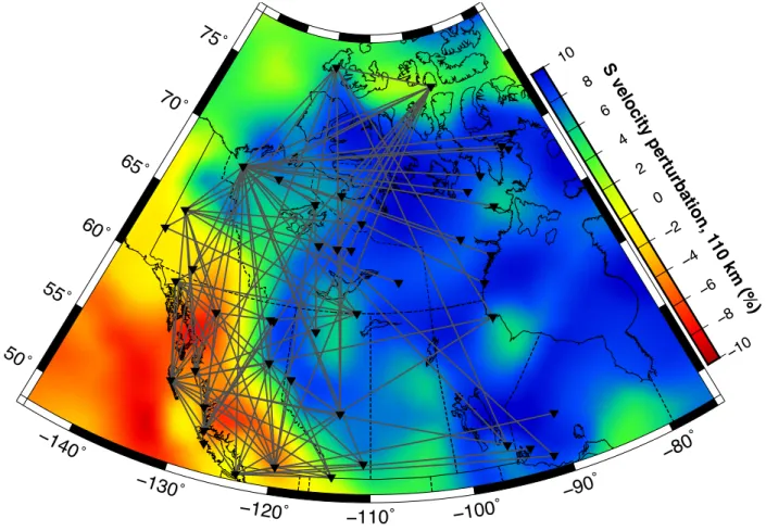
444
Figure 2: Two-station paths (grey lines) analyzed in this study. Background is seismic S velocity 445
at 110 km depth, from the tomographic model of Schaeffer and Lebedev (2014). 446
447 0 1000 2000 3000 4000 5000 6000 7000 0 1000 2000 3000 4000 5000 6000 7000 Time (s) Time (s) a) DLBC trace b) FNBB trace c) Cross-correlation d) Dispersion 0.10 0.08 0.06 0.04 0.02 0.10 0.08 0.06 0.04 0.02 0.10 0.08 0.06 0.04 0.02 F re q u e n c y ( H z ) F re q u e n c y ( H z ) F re q u e n c y ( H z ) P h a s e v e lo c it y ( k m /s ) -1000 -800 -600 -400 -200 0 200 400 600 800 1000 Lag (s) 0.02 0.00 7 6 5 4 3 2 0.04 0.06 0.08 0.10 Frequency (Hz) Starting model
Correlated power spectrum
Possib le disp
ersion curves
Figure 3: Two-station analysis for an event recorded at DLBC (Dees Lake, British Columbia) 448
and FNBB (Fort Nelson, British Columbia). Individual traces (a, b) are shown along with a time-449
frequency analysis; the thin white line indicates group arrival time. The two traces are cross-450
correlated (c) and the cross-correlation phase determines possible Rayleigh phase-velocity curves 451
(d, blue lines). Due to the 2nπ-radian ambiguity of phase, curves are closely spaced at high 452
frequencies; at lower frequencies, only one is plausible (thick line) and may be followed to 453
higher frequency. Here, the curve is usable from ≈ 0.02 to 0.07 Hz. 454
455
Figure 4: Average phase-velocity dispersion curves for all paths examined in this study. The 456
curves are coloured based on the midpoint longitudes of the corresponding two-station paths. 457
458
Figure 5: Phase velocities at four representative periods, plotted as shaded lines along the 459
corresponding two-station great-circle paths. Note that the colour scale differs between panels. 460
461
Figure 6: Checkerboard resolution tests for phase-velocity tomography, at three representative 462
periods. Greyed-out model cells were not sampled by rays. The colour scale is the same for all 463
plots. 464
465
Figure 7: Recovered Rayleigh phase-velocity maps at six periods. The colour scale varies 466
between plots. Black lines are tectonic boundaries from Figure 1. 467
468
Figure 8: Synthetic tests of depth resolution. The input model (solid grey) contains a perturbation 469
from the background (grey dotted); the recovered model (black dashed) is the result of 470
generating synthetic data from the input model, then inverting the result. 471
472
Figure 9: Locations of transects (red lines) inverted to form cross-sections. Yellow dots mark 473
100 km intervals. The blue lines are tectonic boundaries from Figure 1. 474
Figure 10: Example of the cross-section generation process for transect AA-AA’. A 476
pseudosection (top) is extracted from dispersion maps, then each column is inverted separately to 477
form a 1-D model. Concatenation of these 1-D models generates a cross-section, presented in 478
terms of relative (middle) or absolute (bottom) velocity; the base model is IASP91. 479
Figure 11: Three relative-velocity cross-sections perpendicular to the Cordillera-craton 481
boundary, ordered from north to south. Labels at the top of each indicate the tectonic provinces 482
sampled. Letters indicate features discussed in text; dashed line indicates approximate 0% 483
contour between features A and B. 484
485
Figure 12: Additional relative-velocity cross-sections along the strike of the Cordillera (top) and 486
across a high-velocity feature (C) near Great Slave Lake. 487