Measuring Unemployment Insurance Generosity

Pallage: Département des sciences économiques, Université du Québec à Montréal and CIRPÉE Scruggs: Department of Political Science, University of Connecticut

Zimmermann: Corresponding author. Department of Economics, University of Connecticut, 341 Mansfield Road, Unit-1063, Storrs CT 06269-1063, USA

christian.zimmermann@uconn.edu

Cahier de recherche/Working Paper 09-21

Measuring Unemployment Insurance Generosity

Stéphane Pallage Lyle Scruggs

Christian Zimmermann

Abstract:

Unemployment insurance policies are multidimensional objects. They are typically defined by waiting periods, eligibility duration, benefit levels and asset tests when eligible, which make intertemporal or international comparisons difficult. To make things worse, labor market conditions, such as the likelihood and duration of unemployment matter when assessing the generosity of different policies. In this paper, we develop a methodology to measure the generosity of unemployment insurance programs with a single metric. We build a first model with such complex characteristics. Our model features heterogeneous agents that are liquidity constrained but can self-insure. We then build a second model that is similar, except that the unemployment insurance is simpler: it is deprived of waiting periods and agents are eligible forever with constant benefits. We then determine which level of benefits in this second model makes agents indifferent between both unemployment insurance policies. We apply this strategy to the unemployment insurance program of the United Kingdom and study how its generosity evolved over time.

Keywords: Social policy, generosity, unemployment insurance, measurement

1

Introduction

Because of their many dimensions, labor market policies cannot easily be compared through time and space. Their generosity is not easily measured by any known aggregate statistic. Some programs can be restrictive in their access but very supportive of those admitted, while others are open to all, but distribute pennies. To make things worse, this generosity of labor market policies cannot be assessed independently from the economic environment in which they are applied at a given time. In a labor market with full employment, it does not really matter whether support for the jobless is very restrictive. It would, however, in a world in which unemployment is significant. This calls for a strategy of measurement that goes beyond a more or less complex aggregation of program parameters. It should take into account the effect of the program on the welfare of agents and their response to it.

In this paper, we want to contribute to a better understanding of how generous, in an aggregate sense, some labor market policies are relative to one another. We focus on un-employment insurance [UI], but the methodology we propose can be applied to most multi-dimensional social policies. We illustrate our approach with a study of the unemployment insurance program in the United Kingdom whose substantial reform in the 1980s by the Thatcher government has sparked debates on the true effect it had on its overall generos-ity (see, e.g., the slightly different evaluations of Pierson, 1996, and those of Clayton and Pontusson, 1998). The debate on whether social policies have indeed retreated in the 1980s has attracted many researchers in economics and political science. Yet, it is a difficult one, because of the lack of quantitative arguments. Since there are no easy ways to aggregate dimensions of generosity a large place is left to qualitative assessments. Typically, program expenditures are used as the generosity measure. Allan and Scruggs (2004) make the case that replacement ratios be used instead. But they are emphasizing one particular dimension of the package. For a snapshot at the heated debate on the resilience of welfare states, see Pierson (1996), Clayton and Pontusson (1998), Merrien (2002) or Brooks and Manza (2006). Our measurement approach aims at summarizing all dimensions of the unemployment insurance policy into one policy parameter. This methodology can be used for other coun-tries, thus ultimately also to compare different unemployment insurance systems across the world. Clearly, this approach may also be extremely useful to those researchers who wish to

calibrate models with unemployment insurances without accounting for all the dimensions of the actual programs.

We are not the first who seek ways to compare UI systems. Martin (1996), for instance, summarizes a series of results from an OECD research program that publishes international comparisons of UI coverages for various types of workers. Pointwise comparisons of the many dimensions of various social programs can also be found in Scruggs (2006) for a specific type of household. Howell et al. (2007) try to gather labor market institution indicators and aggregate them into a few measures. Closer to our endeavor, Bottero et al. (2004) create a composite indicator of unemployment insurance generosity by taking an unweighted average of indices representing the required contribution period before an unemployment spell, the tax rate covering benefits, the waiting period once unemployed and the replacement rate when eligible for benefits. Quite obviously, this remains a very crude measure of UI generosity. Allard (2005) provides in this respect a more complete exercise. She defines a net reservation wage as the product of the replacement rate, the fraction of a year an agent is eligible and an estimate of the probability of eligibility. The resulting index accounts for some difficult to quantify programmatic demands and sanctions in the course of an unemployment spell.

These measurement attempts, however, use little theory to discipline the indicators, as pointed out by Heckman (2007). Also, they ignore how local labor market conditions may matter. For example, whether the reduction of the eligibility period for UI benefits matters depends on local unemployment duration. Thus while duration of benefits is shorter in the United States than in most European countries, it may not imply that UI programs in the United States are less generous since the duration of unemployment is also shorter. US programs may even be more generous in dimensions that matter more for local labor market. Our approach is one of model-based measurement. We simulate a dynamic general equi-librium model in which we confront two economies, one featuring the complete characteristics of an actual UI program (that of the United Kingdom), the other characterized by a one-dimensional UI program. This single dimension is the level of UI benefits with no time limit or eligibility criterion other than the fact of not having a job offer. The metric by which we measure the overall generosity of an unemployment insurance program is the level of

benefits in the one-dimensional UI program that is socially equivalent, i.e., it reaches the same aggregate welfare value and in this sense makes society indifferent between that and the actual program. Our model features heterogeneous agents and stochastic employment opportunities in the spirit of Hansen and ˙Imrohoro˘glu (1992) and Pallage and Zimmermann (2001, 2005). Agents can self-insure through asset building but face liquidity constraints. There may be moral hazard in the sense that the UI agency may not always be capable of filtering all those who fraudulously apply for benefits. We consider this possibility in our sensitivity analyses.

With this methodology, our measurement captures the effect of possible changes in labor market conditions. It also accounts for the fact that agents’ behavior will likely respond to changes in UI policies or changes in the labor market. Finally, our approach offers a unique way to identify the elements within the policy or the environment that affect most the generosity of unemployment insurance.

Besides the methodological contribution, our paper establishes an important empirical result: unlike commonly believed from a look at replacement rates or from previous mea-surement attempts (e.g. Scruggs, 2006), the actual generosity of the United Kingdom’s UI system has declined substantially and in a sustained way since the 1980s.

In the next sections, we present the modeling strategy. We then calibrate our model to the economy of the United Kingdom, paying special attention to the households, the labor market and the UI policies. We perform simulations and present their results in Section 4. We conclude in Section 5.

2

Modeling strategy

We build two models, comparable in every element but one, the UI policy in place. In the first model, there is a detailed unemployment insurance program, with a vector of characteristics, replacement ratio, eligibility requirements, duration of benefits, etc, that match those in place in the United Kingdom. In the second model, the unemployment insurance is the simplest possible, with a replacement ratio accessible to the jobless as long as they remain so, without any further eligibility clauses. We start by presenting the common parts of both models.

House-holds care about consumption and leisure, which they choose optimally to maximize an in-finite stream of expected, discounted utilities. Savings can be used to self-insure against adverse employment shocks, but there is no borrowing possibility. Every period, households enter an employment opportunity lottery. The outcome of the lottery k is either o if a job offer is made, or n, if not. The households’ likelihood to be given a job offer depends on whether they had such an offer in the period before. In any case, households may choose to accept or turn down a job opportunity. Let x represent the binary labor decision, where x= 1 if a job offer is accepted at time t, 0 if it is refused.

A publicly financed unemployment insurance program provides some income replacement benefits to the unemployed under certain conditions. The UI agency operates with a balanced budget rule. Its revenues are collected from income taxes.

The preferences of a typical household can be represented by the following intertemporal utility function max E0 ∞ X t=1 βtu(ct, lt)

where the periodic utility function u(·) has the usual properties, i.e., it is increasing in each argument and concave; c stands for consumption, l for leisure: lt= 1 for someone who does

not work, lt = 1 − ˆh for someone who works an indivisible amount of time ˆh; β ∈ [0, 1) is

the discount factor.

Savings m from a period to the next evolve in the following way: mt+1 = mt+ ydt − ct, mt≥ 0 ∀t

where yd

t, the disposable income, can have one of three possible values:

yd_t =            (1 − τ )y if employed

(1 − τ )θy if unemployed and eligible to UI (1 − τ )ψy if unemployed and not eligible

with τ , the income tax rate used to raise the revenue necessary to finance the unemploy-ment insurance program. There may be various indicators of eligibility for unemployunemploy-ment insurance benefits. θ and ψ represent income replacement rates. We will call α the vector of UI parameters that will be specified for each model below. Besides replacement rates, α

may also contain eligibility parameters such as waiting period, benefit duration, asset tests, etc. For the time being, we will say that eligibility depends on a vector of variables st that

may follow a potentially endogenous law of motion χ, that is: st+1 = χ(st)

The labor market is stochastic in the following sense. Job opportunities are drawn from a lottery, following a simple binomial Markov process. The probability to be given a job offer at time t thus depends on whether such offer was given at t − 1.

To sum up the household problem, we can write it down in recursive form, using a Bellman equation. For an agent with an employment offer, the relevant Bellman equation is: V(m, s, o; α) = max x x ( max m′ u(c, 1 − ˆh) + β Z k′_|o V(m′, s′, k′; α)d(k′|o) ) +(1 − x) ( max m′ u(c, 1) + β Z k′_|o V(m′, s′, k′; α)d(k′|o) ) S.T. m′ = m + yd_{(s, o, x; α) − c} m′ ≥ 0 s′ = χ(s)

It should be emphasized that when an agent turns down a job offer, he is immediately ineligible for UI.

In a similar fashion, the Bellman equation for an agent without a job offer can be written as: V(m, s, n; α) = max m′ u(c, 1) + β Z k′_|n V(m′, s′, k′; α)d(k′|n) S.T. m′ = m + yd_{(s, n, .; α) − c} m′ ≥ 0 s′ = χ(s)

2.1

Equilibrium

A steady-state equilibrium is an allocation of work, asset and consumption for all agents, a value function V (·), a distribution of assets f (·), and a tax rate τ such that:

1. agents solve their individual intertemporal problems, given (α, τ ) and labor market characteristics;

2. the unemployment insurance agency balances its budget; 3. there is an invariant distribution of agents.

Under this definition of equilibrium, agents in the model assume that the current un-employment insurance and labor market characteristics in any given period will remain unchanged forever. One may question this myopic view of the world. An alternative would be to take into account how agents may be forward looking in these dimensions as well, that is, how they may anticipate changes in the parameters of the UI system and in the unemployment rate and duration. Modeling these expectations, however, is non-trivial. It would make the computation of equilibrium several degrees more difficult, as it would no longer be possible to rely on invariant distributions. We chose the easier path. We do not expect, however, that such policy changes would matter much in terms of expectations, as long as they are not large and are not announced long in advance.

2.2

The simplified UI program

We need to specify α, the rules that govern the simple UI program, its generosity and eligibility criteria. For the simplified UI program, we assume that unemployment benefits can be obtained immediately and that unemployed households stay eligible as long as they remain without a job offer. If eligible, they receive every period the same proportion θ of their income. An agent is ineligible as soon as she turns down a job offer. In that case, she receives a fraction ψ of past income.

This simple UI program thus has the following vector of parameters to which we want to map the detailed UI program:

2.3

The detailed UI program

Next, we want to describe the rules of a real world unemployment insurance policy in as many details as computationally feasible. Such policy typically has the following components:

1. A waiting period a, before the end of which unemployed agents are not eligible for full benefits, although there may be partial benefits in the meantime.

2. The duration of eligibility z, i.e., the number of periods an unemployed agent is entitled to receive benefits.

3. The proportion of past income that unemployed agents obtain as benefits, θ(j), which may vary through the unemployment spell, including the waiting period (j = 1, ..., z). 4. The proportion of income unemployed agents may receive after losing eligibility, ψ, for

example through other social programs.

The vector of policy parameters we need to calibrate from the data is therefore given by: α= (a, z, {θ(j)}j=1,...,z, ψ).

We can now turn to finding those policy parameters for the economy of interest.

3

Parametrization to the United Kingdom

In this first exercise, we want to see how the generosity of the UI program, as summarized by θ in the simplified setup, may change through time. For this purpose, we use the characteristics of α for the United Kingdom for every year, along with the relevant labor market data to parametrize the job-opportunity lottery.

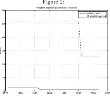
The unemployment benefit system in the UK is summarized in Figures 1 and 2. The details of this system can be confusing because the conditions, and even the names, of its constituent programs have changed several times over the years. Appendix 1 provides a brief overview.1

1

A useful summary of the benefit conditions prior to the early 1980s is provided in Atkinson and Mick-lewright (1985), Chapter 2.

In Figures 1 and 2, “UI benefits” refer to the combined flat-rate and earning-related replacement rates for 1972–1981. The “income security” replacement rate in Figures 1 and 2 is the social assistance benefit. All of the parameters in Figures 1–3 are based on the actual policies in force for the years in question. All figures except for social assistance benefit replacement rates were taken from the summary dataset of the Comparative Welfare State Entitlement Dataset (see Scruggs, 2004). Benefit replacement rates were computed assuming a single-person household with net, in-work wages equal to the average production worker (APW) in the year in which benefits were computed. Benefit rates were based on those in place on April 15 of the year in question. Benefit replacement rates assume a six month unemployment spell, with the six-month total benefit annualized and divided by the net annual wage of the APW. (Annualization facilitates the computation of income tax burdens.) Social assistance replacement rates are taken from the UK’s Department of Work and Pensions as reported by the Institute for Fiscal Studies (2006). Weekly assistance rates (which are not taxable) were simply multiplied by 52 and divided by the net APW wage. The asset test is based on the maximum allowable assets divided by disposable APW.

It is important to bear in mind that, in addition to the phasing out of earnings-related benefits in 1982, UI benefits became taxable in 1983. (Means-tested support benefits, how-ever, are not taxable.) As suggested by Figure 1, making UI benefits taxable made insurance benefits less generous than income support benefits. Note that for this analysis, we used the effective labor income tax rates published by Mendoza, Razin and Tesar (1994), where we complement the published numbers until 1996 with the update available on Enrique Men-doza’s web page. After 1996, we assume no change in the tax rate. One can reasonably argue that these tax rates are too high for our exercise: they are defined as economy-wide average rates, and unemployed workers most likely pay lower tax rates as their income is lower when unemployed and their base income is lower than average. Thus we want to take the parametrizations with and without tax considerations as upper and lower bounds in our measure of UI generosity.2

To calibrate the job market lottery in our model, we make use of the fact that in a binomial Markov process, the probability of receiving a job offer while unemployed is the

2

Note that due to the endogenous response in self-insurance, tax benefits may lower our measure of generosity in some circumstances.

inverse of the unemployment duration. Furthermore, together with the probability of getting a job offer while employed, it determines the unemployment rate Thus, we use time series for the unemployment rate and unemployment duration to parametrize the odds of the lottery in every year. While the unemployment rate is easily available from the United Kingdom’s Office of National Statistics (ONS), obtaining duration data is another matter. We use data on inflows and outflows of UI claimants, again from the ONS, but available only starting in 1989. For the earlier years, we use the numbers published by Layard, Nickell and Jackman (1991, p. 224). Clearly, we would prefer having durations for all unemployed workers. However, using the unemployment rate along with claimant flows gives us durations that should not lie too far from the truth. Atkinson and Micklewright (1985) present evidence for the period 1972–1977 that doing so presents no significant bias, with unemployment duration averaging at 33.4 weeks, while claimant duration is 31.7 weeks. The unemployment rate and duration are presented in Figure 3.

The remaining parameters and functional forms are standard in the literature. Following Hansen and ˙Imrohoro˘glu (1992) and the literature that ensued, we let the utility function be defined as a typical CES function:

u(c, l) = (c

1−σ_lσ₎1−γ

1 − γ − 1

with σ = 0.67 and γ = 2.5. Leisure l is one when unemployed and 0.55 when working. Also, we set the discount factor β in such a way that it corresponds to a discount rate of 4% per year. When running the simulations, we consider the time frequency to be weekly. Such a high frequency is necessary to capture key features of the United Kingdom’s UI policy. The eligibility waiting period, for instance, is one week for part of our sample.

4

Computations and results

Our solution algorithm is as follows. We start by solving numerically the model with the detailed UI program for each year in the sample. This is performed by transforming the state space, in particular assets, m, into a grid, then using discrete dynamic programming techniques to obtain a solution through iterations on the value function. Given the resulting value function, we can extract households’ decisions and infer the invariant distribution of

agent types, f . It is then possible to compute the expected value of a UI program, i.e., the average utility of agents under this program, call it W .

The next step implies solving the model with the simplified UI program using the same technique. We search through various values of θ until we find the one that provides the expected value closest to W , call it θ⋆_{. This θ}⋆ _{is precisely the measure of generosity that we}

seek. This procedure is performed for every year in our 1972–2002 sample, thereby giving us the path of UI generosity over time.

Note that the average value function of the simplified economy is non-monotonic in θ. Indeed, with θ = 0, individuals must bear their employment risk completely and need to self-insure through asset accumulation, which is costly. With θ = 1, income is completely insured, but because agents also value leisure the average agent would tend to prefer a slightly lower θ to preserve the incentives to work and maintain the tax rate reasonably low for those who do. Consequently, there is an optimal θ somewhere in between, and it is unlikely that this optimal θ corresponds to the one we find in the simulation. This means that for any value W that we try to match in the complex economy, there are likely two corresponding θ⋆

in the simple one. This result, analogous to a Laffer curve result, is possibly problematic. In our simulations, however, one of those two replacement rates has always had an unreasonable value (above 100%...).3

We have picked the reasonable one.

It is also theoretically possible for the complex economy to attain a value that is un-reachable by the simple one. For example, if the complex economy has features like those described in Shavell and Weiss (1979) or Hopenhayn and Nicollini (1997), where benefits are optimized as they vary over the unemployment spell or thereafter. While in our experience so far it has not been a problem, it could become one in more generous UI systems than the one studied here.

θ⋆_{, our simulated θ is presented in Figure 4. The figure shows that unemployment}

insurance in the UK became dramatically less generous in the early 1980s and that this trend has continued eversince. Such a result is not self-evident from the parametrization. While progam benefits did decline in a sharp way, the waiting period was reduced and the eligibility to UI was lengthened. It turns out the latter is inconsequential in conjunction

3

Note that a negative value is not inconceivable for low UI benefits and tight asset tests for various benefits, due to the endogenous response in asset accumulation.

with the changes in the labor market.

We can also notice in Figure 4 that our simulated benefits lie most of the time significantly below the program UI benefits. The restrictions to eligibility thus have a significant weight on the generosity of the program. Finally, simulated benefits are much more variable than actual replacement rates, reflecting the changing labor market conditions as well as movements in the other program parameters. Also, early in the sample, some of the variability is due to the fact that generosity was closer to a social optimum, and thus was in a flatter portion of the average value function.

These various influences will be disentangled in the coming pages, but it is important that we first have a look at an alternative, quite intuitive measure of generosity. A “naive” and much simpler way to proceed would be to compute the present value of benefits under the current system and identify the corresponding “permanent income,” ˜θ:

a X t=1 βt−1θt+ a+z X t=a+1 βt−1θt+ ∞ X t=a+z+1 βt−1ψ= 1 1 − βθ.˜

If we compare this naive ˜θ to our simulated θ, we can see in Figure 5, how different a portrait of generosity we would have drawn. While the naive ˜θwould have recorded a decline in UI generosity, it would have in no way registered the huge decrease in the early eighties. Several factors contribute to this mismeasurement: The naive measure is a simple accounting measure. As such, it does not take into account changes in the labor market, it ignores means tests, and it does not factor in how workers’ behavior changed in terms of self-insurance. In particular, the naive measure displays even less of a decline than the program UI benefits. This, we think, speaks loudly in favor of using a general equilibrium-based measure such as ours.

We now turn to analyzing the weight of the various elements within our measure. In other words, what shapes our generosity measure? There are two ways to find an answer to this question: first, by regressing θ⋆ _{on its determinants; second, by performing counterfactual}

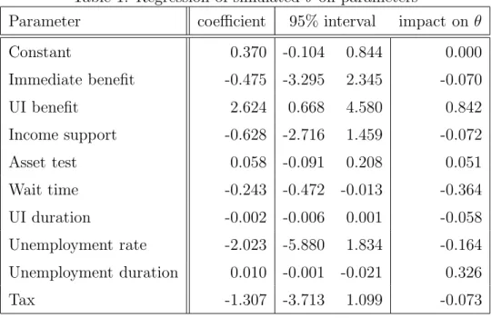
analyses. Table 1 displays the results of the regression. Obviously, this exercise is full of flaws, starting with our small sample and correlated explanatory variables. But the fact that the interval around the coefficients is very large suggests that the relationships may not be linear. Also, some variables could have a large impact. The last column describes

the change in generosity resulting from the smallest to the largest value in the sample. We see that quite expectedly program UI benefits have a strong impact on our measure, but so do waiting times, the unemployment rate and the unemployment duration, and to a lesser extent the other program variables.

We believe, however, that the we could have a much better idea of the various influences using the technology that we have just built. In the coming lines, we evaluate the impact of the program variables and the labor market conditions through counterfactuals using our model. The idea here is to run the same simulations as before, but with modified variables. In Figures 6 to 13, we look in turn at the influence of each variable by setting it to its average value in the sample. Thus, any difference with the benchmark simulation is due to variations in the variable at hand, variations that incorporate the endogenous responses of the model households.

In Figure 6, for instance, the unemployment rate is set for the whole sample period to its average value of 7.46%. While the unemployment rate does not seem to affect the general downward trend of generosity, it seems to affect some of its variablity, in particular in the latter sample period. The reverse is true for UI benefits: they clearly explain the trend in generosity, but not its variability (Figure 7).

Looking further at other variables, we find that the unemployment duration affects some-what the variability of generosity (Figure 8), and that waiting times have virtually no impact (Figure 9) on our measure. Figure 10 shows benefit duration during the last seven years last-ing as long as before the reform, i.e., 52 weeks instead of 26. The generosity does increase, but in a relatively small way. Changes in income security affect outcomes about as much as several of the other variables did (Figure 11).

The impact of tax benefits for unemployed workers is more substantial (as can be seen from Figure 12). Interestingly, for recent years, removing tax benefits improves generosity through the endogenous response of households who revert more to self-insurance and thus rely less on unemployment insurance.

Finally, we see in Figure 13 that the introduction of asset tests that were truly binding has had a rather substantial impact, in particular during the early eighties when benefits were more generous than today.

All in all, these counterfactual experiments show that, except for the waiting period, all changes in labor market conditions and program parameters have a measurable impact on program generosity. It is therefore important to take them all into account for any evaluation of the generosity of an unemployment insurance system.

Other parameter values that are not related to the unemployment insurance program or the labor market conditions, such as risk aversion or the discount rate, may also influence our measure of generosity. However, as a change in such a parameter value would affect both the complex and the simple model economies, the impact is moderate. The strongest impact comes from a change in the risk aversion parameter, as shown in Figure 14.

Moral hazard may also have an impact on the measure of generosity, as workers may choose to shirk differently, depending how generous the system is. But as the generosity would be comparable, by definition, in the complex and simple model economies, this should only have a negligible impact, unless there are some very strong amplification mechanisms at play with asset accumulation. When amending the model with the possibility of moral hazard much in the same way as Hansen and ˙Imrohoro˘glu (1992) and Pallage and Zimmermann (2001), we find that workers do not bother to shirk as the UI system is not sufficiently generous in the case of the UK to risk losing a sure income.

5

Conclusion

We view the main contribution of this paper as methodological. We develop a method to de-termine a comparable one-dimensional measure of the level of generosity of a social program, in our case the unemployment insurance, based on a micro-founded model. Specifically, we build a model where heterogeneous agents face labor market shocks, react by accumulating assets and use a multi-dimensional UI system. We then determine how generous a one-dimensional UI system needs to be for society to be indifferent between the two.

Our second contribution is empirical. Parametrizing our model economies to the period 1972–2002 in the United Kingdom, we find dramatic drops in the generosity in the early 1980s despite more generous UI eligibility. Since then, the generosity of unemployment insurance in the UK has continued to decline. We show that the severity of this drop would not have been captured by a measure of generosity that would have focused solely on the parameters

of the system, thereby ignoring the reactions of the agents and the changing labor market. The methodology we have presented here can be applied in many ways. For example, it makes it possible to have direct international comparisons of unemployment insurance or other social programs. Is the United States more or less generous than France or Spain when it comes to supporting the jobless? The answer to such question should be of high interest to policy makers and to researchers trying to understand differences in employment incentives across countries (see, e.g. Ljundqvist and Sargent, 1998). Others may find our measures of interest for the proper calibration of unemployment insurance benefits in models that necessarily need to abstract from the many dimensions of actual programs. For example, Hagedorn and Manovskii (2008) have emphasized that high benefits (in the order of 90%) can explain the unemployment volatility puzzle brought forward by Shimer (2005). Our measures indicate that the effective generosity is nowhere near this number.4

4

See Pallage, Scruggs and Zimmermann (forthcoming) for an application of the methodology presented here to a comparison of France and the United States.

References

Allan, James P. and Scruggs, Lyle, 2004. “Political Partisanship and Welfare State Reform in Advanced Industrial Societies,” American Journal of Political Science, vol. 48(3), pages 496–512, July.

Allard, Gayle, 2005. “Measuring the Changing Generosity of Unemployment Benefits: Beyond Existing Indicators,” Instituto de Empresa Business School Working Paper 05-18.

Atkinson, A. B. and Micklewright, John, 1985. “Unemployment Benefits and Unemployment Duration: A Study of Men in the United Kingdom in the 1970s,” London: Suntory-Toyota International Center for Economics and Related Disciplines.

Botero, Juan, Djankov, Simeon, Porta, Rafael, Lopez-De-Silanes, Florencio and Shleifer, An-drei, 2004. “The Regulation of Labor,” The Quarterly Journal of Economics, vol. 119(4), pages 1339–1382, November.

Brooks, Clem and Manza, Jeff, 2006. ”Why DoWelfare States Persist?” The Journal of Politics, vol. 68(4), pages 816–827, November.

Clayton, Richard, and Pontusson, Jonas, 1998. “Welfare-State Retrenchment Revisited: Enti-tlement Cuts, Public Sector Re- structuring, and Inegalitarian Trends in Advanced Capi-talist Societies,” World Politics, vol. 51, pages 67–98, October.

Hagedorn, Marcus, and Manovskii, Iourii, 2008. “The Cyclical Behavior of Equilibrium Un-employment and Vacancies Revisited,” American Economic Review, American Economic Association, vol. 98(4), pages 1692–1706, September .

Hansen, Gary D. and ˙Imrohoro˘glu, Ayse, 1992. “The Role of Unemployment Insurance in an Economy with Liquidity Constraints and Moral Hazard,” Journal of Political Economy, University of Chicago Press, vol. 100(1), pages 118–42, February.

Heckman, James, 2007. “ Comments on Are Protective Labor Market Institutions at the Root of Unemployment? A Critical Review of the Evidence by David Howell, Dean Baker, Andrew Glyn, and John Schmitt,” Capitalism and Society, bePress, vol. 2(1), article 5. Hopenhayn, Hugo A and Nicolini, Juan Pablo, 1997. “Optimal Unemployment Insurance,”

Journal of Political Economy, University of Chicago Press, vol. 105(2), pages 412–438, April.

Howell, David R., Baker, Dean, Glyn, Andrew and Schmitt, John, 2007. “Are Protective Labor Market Institutions at the Root of Unemployment? A Critical Review of the Evidence,” Capitalism and Society, bePress, vol. 2(1), article 1.

Institute for Fiscal Studies, 2006. “Fiscal Facts: Benefit Tables for Income Support and Sup-plementary Benefits.” Updated March 2006. http://www.ifs.org.uk/ff/ indexben.php (Ac-cessed June 10, 2007)

Layard, Richard, Nickel, Stephen, and Jackman, Richard, 1991. “Unemployment: Macroeco-nomic Performance and the Labour Market,” Oxford University Press.

Ljungqvist, Lars and Sargent, Thomas J., 1998. “The European Unemployment Dilemma,” Journal of Political Economy, University of Chicago Press, vol. 106(3), pages 514–550, June.

Martin, John P., 1996. “Measures of Replacement Rates for the Purpose of International Comparisons: A Note,” OECD Economic Studies, OECD, number 26, pages 99–115. Mendoza, Enrique, Razin, Assaf and Tesar, Linda, 1994. “Effective tax rates in

macroeco-nomics: Cross-country estimates of tax rates on factor incomes and consumption,” Journal of Monetary Economics, vol. 34(3), pages 297–323, December.

Merrien, Francois-Xavier, 2002. “Etats-providence en devenir: Une relecture critique des recherches recentes,” Revue fran¸caise de sociologie, vol. 43, No. 2, L’Europe sociale en perspectives (Apr. - Jun.), pages 211–242

Pallage, St´ephane, Scruggs, Lyle and Zimmermann, Christian, forthcoming. “Unemployment Insurance Generosity: A Trans-Atlantic Comparison,” Annales d’ ´Economie et de Statis-tique.

Pallage, St´ephane and Zimmermann, Christian, 2001. “Voting on Unemployment Insurance,” International Economic Review, vol. 42(4), pages 903–23, November.

Pallage, St´ephane and Zimmermann, Christian, 2005. “. Heterogeneous Labor Markets and the Generosity Towards the Unemployed: An International Perspective.” Journal of Com-parative Economics, vol. 33(1), pages 88–106, March.

Pierson, Paul, 1996. “The New Politics of the Welfare State,” World Politics, vol. 48, 143-79. Scruggs, Lyle, 2004. “Welfare State Entitlements Data Set: A Comparative Institutional Analysis of Eighteen Welfare States,” Version 1.0b, http://sp.uconn.edu/ ∼scruggs/wp.htm (Accessed June 10, 2007)

Scruggs, Lyle, 2006. “The Generosity of Social Insurance, 1971–2002,” Oxford Review of Eco-nomic Policy, Oxford University Press, vol. 22(3), pages 349–364, Autumn.

Shavell, Steven and Weiss, Laurence, 1979. “The Optimal Payment of Unemployment Insur-ance Benefits over Time,” Journal of Political Economy, University of Chicago Press, vol. 87(6), pages 1347–1362, December.

Shimer, Robert, 2005. “The Cyclical Behavior of Equilibrium Unemployment and Vacancies,” American Economic Review, American Economic Association, vol. 95(1), pages 25–49, March.

A

A brief description of the United Kingdom’s

unem-ployment benefit system

Like most European countries, the unemployment benefit system in the UK consists of an insurance benefit available to all insured individuals who are unemployed, together with a means-tested assistance benefit and a housing benefit available to those with low income and limited means. A rare feature of the contemporary UK system is that the contribution-based benefit is paid at a flat rate, and is equal to the income-based benefit.

Insurance. A constant element of Britain’s unemployment insurance benefit since the end of the second World War is the flat rate (or contribution-based) benefit. From 1948 to 1995, this was called simply Unemployment Benefit. In 1995, the name changed to Contribution-Based Jobseekers Allowance (JSA). The level of this benefit has changed an-nually (sometimes more frequently during periods of high inflation) to reflect changes in living standards.5

Historically, this benefit has been paid after a three day waiting period. Until 1996, this benefit was payable for up to 52 weeks. From 1996 on, the duration of the benefit was reduced to 26 weeks. Between 1966 and 1981, the flat rate amount was supplemented by an earnings-related benefit. The earnings related supplement varied with the worker’s wage level. When in force, it was paid for up to 26 weeks, after a 12 day (two week) waiting period. When originally introduced in 1966, the earnings-related supplement was 33% of weekly wagesbetween 9 and 30 pounds per week. From 1974, the 33% band applied to weekly wages between 10 and 30 pounds, and a second band was introduced(15% of wages between 30 and 48 pounds). Under the Thatcher government, the earnings-related benefit was gradually eliminated between 1980 and 1982. Between 1980 and 1982, moreover, the earnings-related formula was pared back slightly.

Social Assistance. While unemployment insurance is paid to the insured unemployed regardless of their income, social assistance benefits are means-tested, and they have no time limits. Social assistance benefits for the unemployed have also undergone two major reorganizations. Until 1988, they were known as Supplementary Benefits. In that year,

5

In addition, the flat rate benefit is adjusted based on age (over/under 18 or 25), family circumstances, such as whether the household of the claimant has a dependent spouse or children, and, under JSA, disability.

they became known as Income Support. Since 1995, however, they have been known as Income-based Jobseekers Allowance. Despite these reorganizations, the basic conditions and amounts paid for these benefits have been regularly adjusted in line with inflation and wages. As a rule, those on unemployment insurance are not eligible for social assistance for themselves. However, under existing rules, they might qualify for social assistance benefits for dependents.

Housing benefit. A final notable benefit available to the unemployed is the housing allowance. The latter is a means-tested benefit designed to cover parts of the costs of rental housing up to the full amount of rent (subject to a maximum “reasonable” rent). All UK residents, including those employed or receiving contribution-based JSA, are eligible for housing allowance provided they meet the means-test.

A final note about unemployment insurance benefits is that, until 1982, they were not considered taxable income. In that year, unemployment benefits were made taxable. To-day, only contribution-based job seekers allowances are taxable. All means-tested benefits, including housing benefit, are not taxable.

Table 1: Regression of simulated θ on parameters

Parameter coefficient 95% interval impact on θ

Constant 0.370 -0.104 0.844 0.000 Immediate benefit -0.475 -3.295 2.345 -0.070 UI benefit 2.624 0.668 4.580 0.842 Income support -0.628 -2.716 1.459 -0.072 Asset test 0.058 -0.091 0.208 0.051 Wait time -0.243 -0.472 -0.013 -0.364 UI duration -0.002 -0.006 0.001 -0.058 Unemployment rate -2.023 -5.880 1.834 -0.164 Unemployment duration 0.010 -0.001 -0.021 0.326 Tax -1.307 -3.713 1.099 -0.073 Figure 1: 1970 1975 1980 1985 1990 1995 2000 2005 10 20 30 40 50 60 70 80 90 100 110 %

Program benefit parameters, as % of average income, with tax benefits immediate benefits UI benefits income support asset test

Figure 2: 19700 1975 1980 1985 1990 1995 2000 2005 10 20 30 40 50 60 weeks

Program eligibility parameters, in weeks

waiting period UI eligibility period Figure 3: 19700 1975 1980 1985 1990 1995 2000 2005 5 10 15 20 25 30 35 40 45 %, weeks

Labor market parameters

unemployment rate unemployment duration

Figure 4: 19705 1975 1980 1985 1990 1995 2000 2005 10 15 20 25 30 35 40 45 %

Effective UI coverage in simulated economies

simulated benefits UI benefits Figure 5: 19705 1975 1980 1985 1990 1995 2000 2005 10 15 20 25 30 35 40 45 %

Comparison of simulated and naive effective UI coverage with tax benefits naive simulated

Figure 6: 19705 1975 1980 1985 1990 1995 2000 2005 10 15 20 25 30 35 40 45 %

Robustness tests on UI coverage

average unemployment benchmark Figure 7: 19705 1975 1980 1985 1990 1995 2000 2005 10 15 20 25 30 35 40 45 %

Robustness tests on UI coverage

average benefits benchmark

Figure 8: 19705 1975 1980 1985 1990 1995 2000 2005 10 15 20 25 30 35 40 45 50 55 %

Robustness tests on UI coverage

av. unemp duration benchmark Figure 9: 19705 1975 1980 1985 1990 1995 2000 2005 10 15 20 25 30 35 40 45 %

Robustness tests on UI coverage

constant wait time benchmark

Figure 10: 19705 1975 1980 1985 1990 1995 2000 2005 10 15 20 25 30 35 40 45 %

Robustness tests on UI coverage

constant benefit duration benchmark Figure 11: 19705 1975 1980 1985 1990 1995 2000 2005 10 15 20 25 30 35 40 45 %

Robustness tests on UI coverage

average income security benchmark

Figure 12: 19705 1975 1980 1985 1990 1995 2000 2005 10 15 20 25 30 35 40 45 %

Robustness tests on tax benefits

no benefits with benefits (benchmark)

Figure 13: 19705 1975 1980 1985 1990 1995 2000 2005 10 15 20 25 30 35 40 45 %

Robustness tests on UI coverage on asset test

no asset test benchmark

Figure 14: 19705 1975 1980 1985 1990 1995 2000 2005 10 15 20 25 30 35 40 45 50 %

Robustness tests on risk aversion

ρ=1.5 ρ=2.5 (benchmark)