On Portfolio Choice, Liquidity, and Short Selling: A Nonparametric Investigation

Texte intégral

(1)2003s-27. On Portfolio Choice, Liquidity, and Short Selling: A Nonparametric Investigation Eric Ghysels, João Pereira. Série Scientifique Scientific Series. Montréal Mai 2003. © 2003 Eric Ghysels, João Pereira. Tous droits réservés. All rights reserved. Reproduction partielle permise avec citation du document source, incluant la notice ©. Short sections may be quoted without explicit permission, if full credit, including © notice, is given to the source..

(2) CIRANO Le CIRANO est un organisme sans but lucratif constitué en vertu de la Loi des compagnies du Québec. Le financement de son infrastructure et de ses activités de recherche provient des cotisations de ses organisationsmembres, d’une subvention d’infrastructure du ministère de la Recherche, de la Science et de la Technologie, de même que des subventions et mandats obtenus par ses équipes de recherche. CIRANO is a private non-profit organization incorporated under the Québec Companies Act. Its infrastructure and research activities are funded through fees paid by member organizations, an infrastructure grant from the Ministère de la Recherche, de la Science et de la Technologie, and grants and research mandates obtained by its research teams. Les organisations-partenaires / The Partner Organizations PARTENAIRE MAJEUR . Ministère des Finances, de l’Économie et de la Recherche [MFER] PARTENAIRES . Alcan inc. . Axa Canada . Banque du Canada . Banque Laurentienne du Canada . Banque Nationale du Canada . Banque Royale du Canada . Bell Canada . Bombardier . Bourse de Montréal . Développement des ressources humaines Canada [DRHC] . Fédération des caisses Desjardins du Québec . Gaz Métropolitain . Hydro-Québec . Industrie Canada . Pratt & Whitney Canada Inc. . Raymond Chabot Grant Thornton . Ville de Montréal . École Polytechnique de Montréal . HEC Montréal . Université Concordia . Université de Montréal . Université du Québec à Montréal . Université Laval . Université McGill ASSOCIÉ AU : . Institut de Finance Mathématique de Montréal (IFM2) . Laboratoires universitaires Bell Canada . Réseau de calcul et de modélisation mathématique [RCM2] . Réseau de centres d’excellence MITACS (Les mathématiques des technologies de l’information et des systèmes complexes). Les cahiers de la série scientifique (CS) visent à rendre accessibles des résultats de recherche effectuée au CIRANO afin de susciter échanges et commentaires. Ces cahiers sont écrits dans le style des publications scientifiques. Les idées et les opinions émises sont sous l’unique responsabilité des auteurs et ne représentent pas nécessairement les positions du CIRANO ou de ses partenaires. This paper presents research carried out at CIRANO and aims at encouraging discussion and comment. The observations and viewpoints expressed are the sole responsibility of the authors. They do not necessarily represent positions of CIRANO or its partners.. ISSN 1198-8177.

(3) On Portfolio Choice, Liquidity, and Short Selling: A Nonparametric Investigation* Eric Ghysels†, João Pereira‡. Résumé / Abstract Nous estimons des décisions de choix de portefeuille en fonction de mesures de liquidité à l'aide de méthodes non paramétriques. Nous trouvons que les parts optimales de portefeuilles sont surtout influencées par la liquidité pour des horizons à court-terme. Par ailleurs, ces parts optimales sont toujours positives, ce qui pourrait expliquer le peu de vente à découvert observé sur le marché américain. Mots clés : choix de portefeuille, liquidité, vente à découvert. This paper studies the time series effect of changes in liquidity on optimal portfolio allocations. Using a nonparametric approach, we are able to handle models that are analytically intractable. Specifically, we directly estimate optimal portfolio weights for a CRRA investor as functions of liquidity. Liquidity is measured by turnover, dollar volume, or price impact. We consider three different investment horizons: daily, weekly, and monthly. Using a sample of NYSE stocks from 1963-2000, we document a very interesting temporal dimension to the effects of changes in liquidity: whereas optimal weights are strongly increasing functions of liquidity at the very short daily and weekly horizons, they become decreasing functions of liquidity at longer monthly horizons. Overall, the dependence of optimal weights on liquidity is most noticeable for small stocks at short investment horizons. Finally, the optimal conditional portfolio weights documented in this paper are never negative, which may help explain the low level of short selling observed in the US stock market. Keywords: portfolio choice, liquidity, short-selling.. * We are grateful to Jennifer Conrad, Adam Reed, Harold Zhang, and seminar participants at UNC-Chapel Hill for helpful comments. We also thank Michael Brandt for providing software code. Department of Economics, University of North Carolina and CIRANO, Gardner Hall CB 3305, Chapel Hill, NC 27599-3305, tel.: (919) 966-5325, e-mail: eghysels@unc.edu. ‡ Kenan-Flagler Business School, University of North Carolina, McColl Bldg CB 3490, Chapel Hill, NC 275993490, tel.: (919) 962-3154, e-mail: Joao Pereira@unc.edu. Financial support from the Portuguese Science and Technology Foundation is gratefully acknowledged. †.

(4) 1. Introduction. How does an asset’s liquidity affect its demand? A substantial amount of research effort has been devoted to the relation between liquidity and the conditional distribution of returns. However, the question of how liquidity influences portfolio allocations is not easy to address, particularly since for most interesting utility functions — like the widely used power utility — portfolio weights are complex implicit functions of higher-order conditional moments of returns. The goal of this paper is to characterize the dependence of optimal portfolio choices on changes in the liquidity of assets through time. The dependence of portfolio weights on liquidity is not the only challenging issue, as liquidity itself is a complex and not easy to measure concept. A possible, even though relative, definition would be to say that an asset is liquid if large quantities can be traded in a short period of time without moving the price too much. Accordingly, several alternative measures of liquidity have been used in the literature, including the price impact of trade, the bid-ask spread, share or dollar volume, and turnover, among others. A security is taken to be more liquid the lower its price impact, the tighten its bid-ask spread, or the higher its volume or turnover. The standard cross sectional empirical finding is that expected returns are decreasing in liquidity, as measured by the bid-ask spread in Amihud and Mendelson (1986), turnover in Datar, Naik, and Radcliffe (1998), price impact in Brennan and Subrahmanyan (1996), or trading volume in Brennan, Chordia, and Subrahmanyan (1998). The reasoning is that investors anticipate having to pay higher transaction costs when they need to sell the illiquid assets in the future, and thus require a higher expected return to hold them. However, empirical evidence on the time series relation is quite different. Whereas Amihud (2002) finds a long-term (monthly and yearly) negative relation between market liquidity (measured by price impact) and market returns, Gervais, Kaniel, and Mingelgrin (2001) find a short-term (up to 20 days) positive relation between liquidity (measured by volume) and stock returns. Hence, it appears: (1) that there is a temporal dimension to the effects of changes in liquidity, with expected returns increasing in liquidity at short daily or weekly frequencies, while decreasing at longer monthly or yearly frequencies; and/or (2) that different measures. 2.

(5) of liquidity produce significantly different forecasts of the first moment of returns. There is little guidance from theory on how portfolio weights should respond to liquidity. In a recent paper, Longstaff (2001) associates illiquidity with the notion of thin markets, i.e., with the possibility that sometimes investors may find it impossible to initiate or unwind positions in a given security at any price. Thus, he defines illiquidity as a bound on the amount of shares that can be traded per period. Specifically, Longstaff analyzes a continuoustime portfolio choice model in which a logarithmic-utility investor is restricted to trading strategies of bounded variation. Through numerical examples, Longstaff shows that in general the investor chooses a lower initial portfolio weight in the presence of liquidity constraints. Furthermore, he shows that the required price discounts to induce investors to hold illiquid securities can be substantial. Our contribution is to analyze the empirical relation between optimal portfolio allocations and different measures of liquidity, at different investment frequencies. We extend the previous papers by studying the optimal portfolio functions themselves, instead of focusing only on the first conditional moment of returns. We adopt the nonparametric method of Brandt (1999) and A¨ıt-Sahalia and Brandt (2001). This technique allows us to express optimal portfolio choices directly as functions of the state variable, i.e. liquidity, without requiring the intermediate step of estimating conditional moments of returns. We test three different measures of liquidity: Turnover, Dollar Volume, and Price Impact. We also include Signed Turnover, which does not measure liquidity directly, but can be thought of as a proxy for order flow. To address the time dimension of liquidity, we consider investment decisions of a power-utility investor with three different horizons: one day, one week, and one month. Since the previous papers found that liquidity is more strongly related to the returns of small than large firms, we also separate the analysis between these two classes of stocks. Using a sample of NYSE stocks from 1963 to 2000, we find optimal conditional portfolio functions consistent with the previous papers. First, and most surprisingly, we do indeed find an inversion in the relation between optimal portfolio weights and liquidity across frequencies: whereas optimal weights are strongly increasing functions of liquidity at the very short daily and weekly horizons, they become decreasing functions of liquidity at longer monthly horizons. While we do not have a theoretical explanation for this fact, it is consistent with the findings 3.

(6) in Gervais, Kaniel, and Mingelgrin (2001) and Amihud (2002). It seems that increases in liquidity induce prices to adjust upward, to reduce the illiquidity discount found in Longstaff (2001), and once the adjustment is done, after a few days, expected returns become lower (consistently with cross-sectional well-documented facts). Since we compute optimal weights, rather than individual moments, our results would further imply that this short-term price run up is not accompanied by increases in conditional moments that the investor dislikes. In particular, it must be the case that, during this short period of price run up, the investor forecasts a relatively high first moment and a relatively low variance of returns. Secondly, we find that the three measures of liquidity tested do not produce exactly the same results: the reversal mentioned above is visible in Dollar Volume, less so in Price Impact, and not so in Turnover. On the other hand, Turnover is a stronger determinant of optimal weights at shorter frequencies. Thirdly, not surprisingly, we find a stronger relation between liquidity and optimal weights for small than for large stocks. Finally, we document a very strong dependence of portfolio weights on Signed Turnover. Along a quite different dimension, our study may help to explain the “intriguing short sales reluctance puzzle” mentioned in D’Avolio (2002, p. 303). This author shows that most stocks are shortable: stocks potentially impossible to short account for less than 1% of the market value; 91% of actually borrowed stocks have an average loan fee of only 0.17% per annum. Geczy, Musto, and Reed (2002) show that short-selling costs are sufficiently low to allow for the profitable implementation of several well-known trading strategies. However, as documented in Almazan, Brown, Carlson, and Chapman (2002), of all investment funds permitted to engage in short selling, only 10% actually do. Furthermore, the total short interest is typically only 1.5% of market value. Our results show that optimal portfolio weights (conditional on several measures of liquidity) are never negative. That is, a CRRA investor forming his optimal (expected utility maximizing) decisions on basis of liquidity information would never choose to short sell stocks. Hence, our results suggest that investors do not engage in frequent short selling simply because it is not optimal to do so. The next section defines and motivates the liquidity measures used in this paper, section 3 presents our method and data, section 4 the main results, and section 5 concludes.. 4.

(7) 2. Conditioning information. This section defines and motivates the use of liquidity measures. Note that most of the papers referred below deal with the relation between liquidity and the first or second conditional moments of returns. However, we stress that we are only implicitly interested in conditional moments of returns, since the nonparametric technique used allows for the direct estimation of optimal portfolio functions. Nevertheless, these relations can help us rationalize the shape of the portfolio functions found — any risk-averse investor obviously likes higher means and lower variances. We examine Turnover in a first subsection, followed by Dollar Volume, and then by Price Impact. The last subsection introduces Signed Turnover.. 2.1. Turnover. The first measure of liquidity is Turnover, defined for an individual security as Vi /Ni , where Vi is the share volume of security i and Ni the number of shares outstanding. For a portfolio, we define Turnover (TURN) as the value-weighted average. T U RN ≡. I X i=1. ωi. Vi Ni. where I is the number of securities in the portfolio, and ωi ≡ Ni Pi /. PI. j=1 Nj Pj ,. with Pi being. the stock price. Datar, Naik, and Radcliffe (1998) propose turnover as a proxy for liquidity and, in an exercise similar to Amihud and Mendelson (1986), find that turnover is cross-sectionally negatively related to monthly returns. Jones (2002) builds a long time series from 1900–2000 of large NYSE stocks and finds that high turnover predicts low stock returns one year or more ahead. If changes in turnover can be interpreted as fluctuations in the trading bound defined in Longstaff (2001), then we would expect to see (1) lower turnover accompanied by lower portfolio weights and (2) increases in turnover followed by very short-run price increases as the security price adjusts to its higher liquidity.. 5.

(8) 2.2. Dollar Volume. A second measure of liquidity is Dollar Volume (DVOL), defined for a portfolio as. DV OL ≡. I X. Vi Pi. i=1. Brennan, Chordia, and Subrahmanyan (1998) find that dollar volume is cross-sectionally negatively related to monthly risk-adjusted returns. In the time series dimension, Gervais, Kaniel, and Mingelgrin (2001) find that stocks which experience unusually high (low) volume over a day or a week tend to appreciate (depreciate) over the subsequent 1, 10, and 20 days. They argue that this finding is consistent with the visibility hypothesis: if higher volume attracts attention to a stock, then the number of potential buyers increases and thus the stock price will also tend to increase. They disaggregate the analysis by market capitalization and find that the effect is stronger for small firms than for large firms. Hence, we expect to see portfolio weights increasing in volume, especially at very short investment horizons.. 2.3. Price Impact. Another measure of liquidity is the Price Impact (PI) of trading. In the microstructure literature, this is usually defined as the price change induced by a given signed (buy/sell) order size. Hence, a more liquid security will have a lower price impact. Brennan and Subrahmanyan (1996) find a positive cross-sectional relation between this measure and stock returns. Since high frequency data on transactions and quotes is not available for long periods of time, we follow Amihud (2002) and define a daily stock measure of price impact as the ratio of absolute return (Ri ) to dollar volume. For a portfolio, I. PI ≡. 1 X |Ri | I Vi Pi i=1. Amihud (2002) computes this measure for the whole market and finds a positive time series relation with stock returns at the monthly and yearly frequencies.. 6.

(9) 2.4. Signed Turnover. Finally, we also consider the quantity Signed Turnover (STRN):. ST RN ≡ T U RN × sign(R). where R is the return on the portfolio, and sign(R) is equal to +1 (−1) when R is positive (negative). P´astor and Stambaugh (2001) and Eckbo and Norli (2002) use similar quantities to estimate monthly liquidity measures. Signed Turnover cannot be directly associated with liquidity; yet it is a proxy for (standardized) order flow. We expect it to be positively related to optimal portfolio weights if, conditionally on high turnover, returns display positive autocorrelation. Previous empirical findings on this issue are mixed. Some studies have focused on aggregate returns and volume. Campbell, Grossman, and Wang (1993) found that returns on high-volume days tend to reverse themselves. LeBaron (1992) finds that the return autocorrelation on the Dow Jones index decreases with volume. Other studies focused on individual stock data. Conrad, Hameed, and Niden (1994) found return reversals (continuation) after high (low)-transaction weeks. On the contrary, Stickel and Verrecchia (1994) found return continuation after high-volume days. Llorente, Michaely, Saar, and Wang (2000) advocate that these differences can be explained by the higher degree of information asymmetry present in smaller illiquid stocks. They find that companies with smaller market capitalization, or higher bid-ask spreads, display return continuation following high volume days, whereas larger stocks, or stocks with smaller bid-ask spreads, show almost no pattern in returns following high-volume days. Our results show that Signed Turnover is quite useful in determining portfolio weights for small, illiquid stocks. We find that optimal weights increase in Signed Turnover, which is consistent with the positive autocorrelation hypothesis for small stocks in Llorente, Michaely, Saar, and Wang (2000). Furthermore, we find this same relation for large stocks when the investor rebalances daily — i.e., when even large stocks may have liquidity constraints.. 7.

(10) 3. Econometric estimation of conditional portfolio choices. Consider an investor who maximizes the conditional expected utility of next period’s wealth, subject to budget and adding-up constraints:. max. E[u(Wt+1 )|Zt ]. αt. (1). s.t. Wt+1 = Wt αt0 Rt+1 1 = αt0 ι where Wt is the investor’s wealth at time t, the vector αt ≡ [αt,f. αt,s ]0 represents the pro-. portions of wealth invested in a risk-free asset (αt,f ) and in a portfolio of risky stocks (αt,s ), Rt+1 ≡ [Rt+1,f. Rt+1,s ]0 is the vector of total returns on those assets, ι is a vector of ones, and. Zt represents conditioning information — liquidity, in our case. The investor can have three different horizons, i.e., the difference between t and t + 1 can either be one day, one week, or one year. Assume a utility function with constant relative risk aversion (CRRA):. u(Wt+1 ) =.    W 1−γ / (1 − γ) if γ > 1 t+1  . ln Wt+1. (2). if γ = 1. where γ represents the coefficient of relative risk aversion.1 This utility function is attractive in the sense that the portfolio weights are independent of the level of wealth. However, it has the disadvantage of not permitting a closed-form solution to the investor’s portfolio choice problem. Imposing the adding-up constraint on the weights αt , the first order condition for (1) is: ·. αt,s :. ¸ ∂u(Wt+1 ) E[mt+1 (αt,s )|Zt ] ≡ E (Rt+1,s − Rt+1,f )|Zt = 0 ∂Wt+1. (3). with Wt+1 = Wt [Rf + αt,s (Rt+1,s − Rt+1,f )]. 1. Our empirical results assume a coefficient of relative risk-aversion of γ = 10. Mehra and Prescott (2003) mention that γ = 10 should be considered as an upper bound on the degree of risk-aversion. Even with this number we sometimes find large portfolio weights, but this is just evidence of their well-known equity premium puzzle. For robustness, Section 4.3.1 analyzes the results for different degrees of risk aversion.. 8.

(11) We use the nonparametric estimation technique of Brandt (1999) and A¨ıt-Sahalia and Brandt (2001). It consists of replacing the conditional expectations with sample analogues. To estimate the optimal portfolio weight in a given reference state Z = z¯, we find the number αs (¯ z ) that solves the sample equivalent to the optimality conditions in (3): T. αs (¯ z) :. 1 X 1 mt+1 (αs (¯ z ))k (Zt ; z¯, h) PT =0 Th k (Z ; z ¯ , h) t t=1. (4). t=1. The kernel function k(Zt ; z¯, h) measures how far each sample observation is from the reference point z¯, giving more weight to observations close to z¯. We use a normal kernel: k (Zt ; z¯, h) = ¡ ¢ (2π)−1/2 exp −d2t /2 , with dt = (Zt − z¯)/h, where h is the bandwidth. We apply a standard exactly identified GMM to (4), i.e., αs (¯ z ) is the number that sets the square of the left-hand side of (4) to zero. The choice of the bandwidth h is crucial. A larger h implies averaging across more data points, thus reducing the variance but increasing the bias; a smaller h makes the estimator differentiate more between observations in different states and use fewer points, thus reducing the bias but increasing the variance. The conventional solution to optimize this tradeoff between variance and bias is to choose a bandwidth of the form h = λσ (Z) T −1/(K+4) , where σ (Z) is the standard deviation of the predictor Z, T is the sample size, K is the dimension of Z (one in our case), and λ is a constant. There is no good guidance in the literature for bandwidth selection with non i.i.d. observations, as is the case with our data. For instance, Chaudhuri and Marron (1999) advocate a simple trial and error approach. In our application, a small λ usually produces very noisy portfolio weights that vary a lot with even small changes in liquidity, thus not making much economic sense; a big enough λ will eventually result in a flat portfolio weight, equal to the unconditional estimator. Therefore, we try different values for this constant and pick the one that eliminates local noisy fluctuations but still keeps the basic shape of the portfolio function.2 The main advantage of Brandt’s (1999) approach is that it permits estimating portfolio weights directly from the predictor variables. Whereas traditional studies in conditional port2 The results in Section 4.2 below are for values of λ of 9, 6, and 3 for respectively the daily, weekly, and monthly frequencies. Section 4.3.2 ensures that the results are robust to different values of λ.. 9.

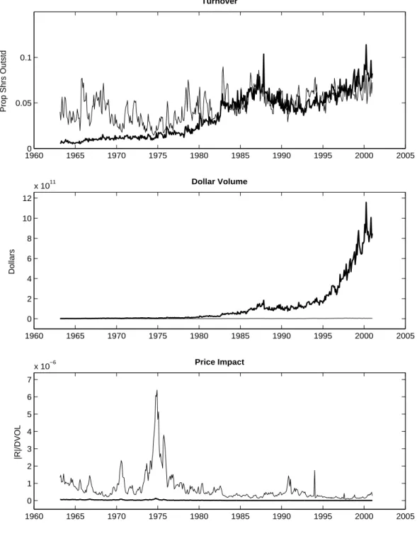
(12) folio choice usually start by estimating a model relating returns to forecasting variables and then find the portfolio weights given the conditional distribution of returns, we perform a single nonparametric estimation relating predictors directly to portfolio weights. The advantage is that we avoid the introduction of additional noise and potential misspecifications from the intermediate step of estimating the return distribution. Being nonparametric, this approach has also the advantage of giving a consistent estimator of the portfolio weights, but has the disadvantage of having higher variance than a correctly specified parametric estimator would have. However, lack of closed-form solutions prevent us from following the latter approach. We conclude this section with a brief discussion regarding the data. We collect daily returns from 1963 to 2000 on three assets: a risk free asset, a portfolio of small stocks, and a portfolio of large stocks. The return on the risk-free asset is the sample average of the return on a one-year Treasury Bill. We form the stock portfolios by sorting the NYSE stocks on their market capitalization. The small stocks portfolio comprises deciles 2 and 3; the large stocks portfolio comprises deciles 9 and 10.3 The daily data is aggregated to weekly and monthly frequencies, resulting in sample sizes of 9431 daily observations, 1978 weekly observations, and 455 monthly observations. We also collect daily volume data from CRSP and compute the measures of liquidity defined above for each of the two stock portfolios. Time-aggregation is done by summing across dates in the cases of Turnover and Dollar Volume, or by averaging across dates in the case of Price Impact. This follows the conventions in Lo and Wang (2000) and Amihud (2002). Figure 1 plots these time series at the monthly frequency. Turnover and Dollar Volume (Price Impact) trend upwards (downwards) and display some extreme positive values. One noteworthy aspect of Figure 1 is that it shows, contrary to what one might expect, that the turnovers of small and large stocks are of the same order of magnitude. This confirms the suggestion of Lo and Wang (2000, p. 272) that “smaller-capitalization companies can have high turnover”. Given that our nonparametric approach requires stationary data, we take the logarithm and detrend each of the predictors. For Turnover, we do a linear detrending of the form:. ln(T U RNt ) = β0 + β1 t + εt 3. (5). The risk-free asset is from www.federalreserve.gov and the stock data is from the Center for Research in Security Prices (CRSP).. 10.

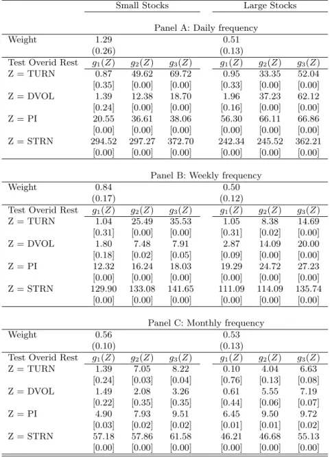
(13) and redefine Turnover (TURN) to be the residual εt of this regression. The time unit t can either be a day, a week, or a month. Similar detrendings are performed for Dollar Volume (DVOL) and Price Impact (PI). For Signed Turnover we do instead an exponential detrending in order to preserve the positive sign of raw Turnover. Hence, we estimate ln(T U RNt ) = β0 eβ1 t ²t. (6). where T U RNt is still the raw Turnover (i.e., before the detrending in (5)), and then redefine Signed Turnover (STRN) to be the product of the residuals ²t of (6) and the sign of returns. We rescale all series by dividing by their standard-deviations to facilitate the interpretation of the results. Table 1 presents descriptive statistics of the four predictors, after detrending and standardizing. By construction, all measures have mean zero and standard-deviation equal to one.. 4. Results. The first subsection presents unconditional portfolio allocations. Section 4.2 provides the mains results on optimal conditional portfolios. The last subsection provides robustness checks.. 4.1. Unconditional portfolio weights. Table 2 presents unconditional portfolio choices. These weights are obtained by applying a standard GMM procedure to the unconditional first order conditions:. αs :. T 1X mt+1 (αs ) = 0 T. (7). t=1. When the risky asset is a portfolio of large stocks, the allocation to stocks is about 0.5, regardless of the investment horizon. For the case of small stocks, the allocation to the risky asset decreases from 1.29 at the daily frequency to 0.56 at the monthly frequency. As a first simple appraisal of whether the unconditional choices are optimal, we use the 11.

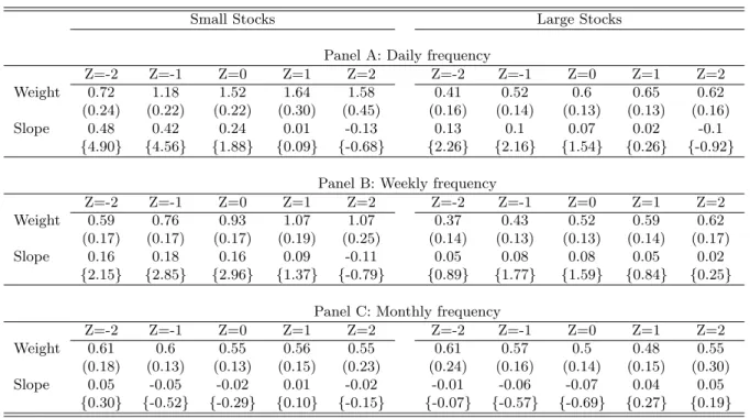
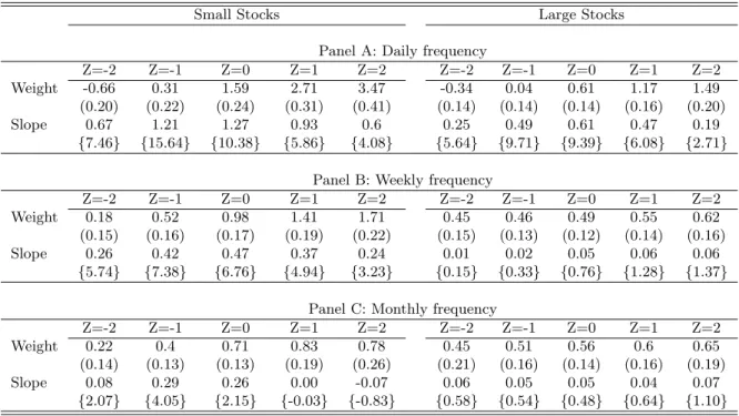
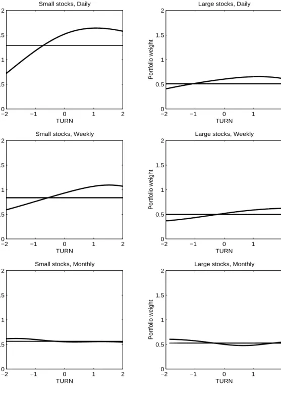
(14) liquidity measures as instruments and re-estimate the resulting overidentified models. In the case where liquidity cannot forecast the return distribution, the unconditional weights are optimal and the resulting unconditional first order conditions are independent of the predictors. Under this null hypothesis, the statistic · X ¸0 ¸ T T 1X −1 1 mt+1 (α) ⊗ g(Zt ) S mt+1 (α) ⊗ g(Zt ) J = min T α T T ·. t=1. (8). t=1. is distributed χ2 with degrees of freedom equal to the size of the vector g(Zt ) minus one. We test several functions of the forecasting variables: g(Zt ) = [1, Zt ], g(Zt ) = [1, Zt , Zt2 ], or g(Zt ) = [1, Zt , Zt2 , Zt3 ]. The optimal matrix S is obtained with the Newey-West estimator. Table 2 presents the χ2 statistic and p-values. At the daily and weekly frequencies, the results overwhelmingly reject that optimal weights are independent of the predictors, suggesting that liquidity is useful in predicting returns at these shorter horizons. At the monthly frequency, while Signed Turnover still seems to be correlated with returns, the other liquidity measures loose some significance, indicating that liquidity becomes less useful at longer horizons.. 4.2. Conditional portfolio weights. We now present the main results of this paper: portfolio weights as functions of liquidity. Each one of the different predictors — Turnover, Dollar Volume, Price Impact, and Signed Turnover — is analyzed in turn. For each of these measures, we present the results in a figure and a corresponding table. Figure 2 shows portfolio choices conditional on Turnover. Each plot shows the proportion allocated to risky assets, αs , as a function of the state variable Z — Turnover in this case. The investor allocates his wealth between a risk-free asset and either a portfolio of small stocks (left column) or a portfolio of large stocks (right column). In the first row the portfolio is rebalanced daily; in the second row, weekly; and in the third, monthly. Table 3 is the companion table to Figure 2. Each panel shows αs (Z), with Z ∈ {−2, −1, 0, 1, 2}, for the corresponding plot in figure 2. Standard errors are obtained with the stationary bootstrap of Politis and Romano (1994). This technique accounts for the autocorrelation in the data and has the advantage, over a simple block bootstrap, of generating a stationary resam-. 12.

(15) pled pseudo-time series.4 The standard errors are presented only to gauge the precision of the nonparametric method used; it is obviously meaningless to test whether a portfolio weight is statistically away from zero.5 The important question is whether the weights respond to changes in liquidity. Hence Table 3 also presents the first derivative of αs (Z), approximated by the finite difference ∂α(Z) ¯¯ α(¯ z + 0.1) − α(¯ z − 0.1) ∼ = ¯ ∂Z Z=¯z 0.2. (9). Stationary bootstrap t-statistics for a zero slope are presented in curly braces below the point estimates. The results show that at the shorter horizons, i.e. daily and weekly, Turnover significantly determines the allocation to small stocks. As Turnover decreases from its average value of zero to -2, the optimal weight on small stocks decreases from 1.52 to 0.72 at the daily frequency, and from 0.93 to 0.59 at the weekly frequency. In this range, all slopes are significant at least at the 10% level. As Turnover increases from zero to positive values, we also see a significant increase in optimal weights, with α(Z = 1) reaching 1.64 (daily) or 1.07 (weekly). However, for higher values of Turnover the weights no longer seem to increase: the slopes at Z=1 and Z=2 are not statistically different from zero. At the longer monthly frequency, optimal portfolio choices do not seem to respond to changes in Turnover. The findings for the case where the risky asset is a portfolio of large stocks are qualitatively similar, but much less pronounced. At the daily frequency, the optimal weight on large stocks still increases with Turnover, but the slopes are only significant at the lower values of Z = −1 and Z = −2. At the weekly frequency, the slope is only significant around Z = −1. At the monthly frequency, again there is no dependence. 4 The algorithm consists of: (1) let the time indices I1 , I2 , ... be a sequence of iid random variables with a discrete uniform distribution on {1, ..., T }; (2) let the block lengths L1 , L2 , ... be a sequence of iid random variables with a geometric distribution; (3) generate pseudo-time series Z ∗ and R∗ by stacking the overlapping blocks, Z ∗ = [ZI1 , ..., ZI1 +L1 −1 , ZI2 , ..., ZI2 +L2 −1 , ...] and similarly for R∗ , stopping when the length of these new series reaches T ; (4) estimate α; (5) repeat B times; (6) compute the standard deviation of the B numbers α. We need to specify the mean of the geometric distribution in step 2, which determines the average block length. Following Horowitz (2000), we set it to T 1/5 . We perform B = 1000 iterations. 5 For another application of the stationary bootstrap see Sullivan, Timmermann, and White (1999). Even though there is some recent research on the asymptotic properties of the bootstrap applied to GMM estimators (for example, Horowitz (2000) and Inoue and Shintani (2001) present cases where the bootstrap provides asymptotic refinements over first-order approximations), little is known about the bootstrap properties when GMM estimators run on top of a kernel function (which is our case).. 13.

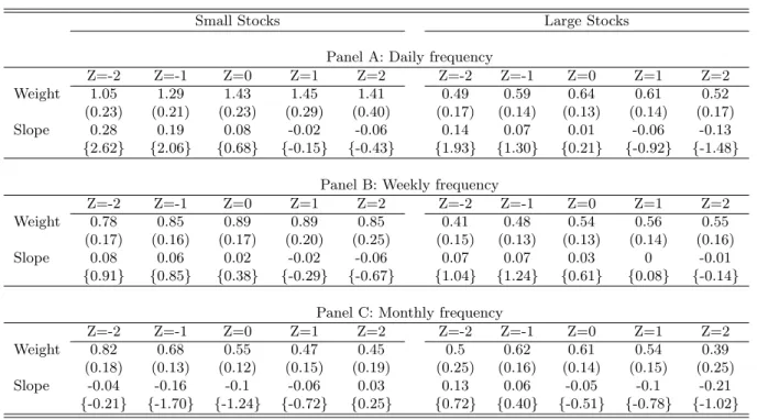
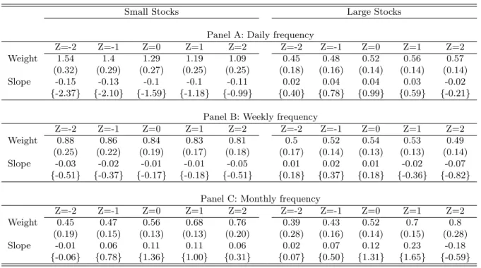
(16) The second measure of liquidity is Dollar Volume. The results are in Figure 3 and Table 4. Overall, Dollar Volume appears to be a somewhat weaker predictor of returns. At the daily frequency, we still see a decrease in αs (Z) for small stocks when Z decreases to -1 or -2; for large stocks, the slope is significant around the Z = −2 level. However, at the weekly frequency, optimal portfolio weights for both classes of stocks do not seem to respond to changes in volume. Quite surprisingly, at the monthly frequency we see small stocks responding again to volume, but now with the inverse sign: the optimal weight decreases with volume. In particular, αs (Z) has a significant negative slope at Z = −1. This finding will be validated in the robustness section below. Figure 4 and Table 5 present the results for Price Impact. Recall that this measure has a different sign than the previous two, i.e., a decrease in Price Impact means that the stocks are becoming more liquid. Overall, the results are similar to the ones with Dollar Volume. For small stocks at the daily frequency, as the Price Impact decreases below the normal value of zero, the weight on small stocks increases. In other words, an increase in liquidity is accompanied by an increase in the optimal portfolio weight. At the weekly frequency αs (Z) is practically flat. For both stocks at the monthly frequency, we see again an inversion of the short-term relation, i.e., αs (Z) becomes decreasing in liquidity. However, the results here are not very strong: while the slope of αs (Z) is significant Z = 1 (large stocks), we do not find evidence of an overall positive first derivative in the robustness section below. Figure 5 and Table 6 show the results for Signed Turnover. This variable magnifies the relations found with simple Turnover, thus appearing to be very relevant conditioning information. Recall that a low negative value of Signed Turnover is associated with high volume originated from heavy selling, whereas a high positive value is associated with high volume caused by heavy buying. At the daily frequency, weights for both small and large stocks are strongly increasing in Signed Turnover, with αs (Z) displaying a very significant positive derivative over the whole range of Z. At the weekly frequency, small stocks still display this strong positive dependence over all values of Signed Turnover, even though the allocation to large stocks becomes insensitive to Z. At the monthly frequency, the optimal weight on small stocks still increases over negative values of Z, which was not visible with normal Turnover. Hence, it seems that distinguishing between turnover in an up and a down market helps 14.

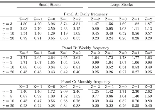
(17) considerably in forecasting the conditional distribution of returns. One remarkable aspect of these results is that the optimal weight on the risky asset is never negative for any of the four predictors studied above.6 This means that short-selling stocks is never optimal for a CRRA investor, given the conditioning information — Turnover, Dollar Volume, Price Impact, and Signed Turnover — studied in this paper. As shown below in section 4.3.1, this result is robust to different degrees of risk aversion.. 4.3. Robustness tests. The next subsection analyzes the effect of different degrees of risk aversion (γ). The last subsection proposes a parametric specification for the portfolio function. 4.3.1. Degree of risk aversion (γ). To analyze whether our conclusions depend on the degree of risk aversion, we re-estimate optimal portfolio weights for γ = 3, γ = 5, and γ = 20. Table 7 presents the results for Price Impact.7 Different degrees of risk-aversion (γ) change mainly the level of the portfolio function (lower γ, higher α), having little effect on the shape of this function. Hence, our conclusions regarding the relation between optimal weights and liquidity variables are not shaped by the level of risk aversion. Furthermore, even with γ = 20, which is an implausible high value, we do not find negative optimal weights on stocks. Hence, our conclusions regarding the non-optimality of short-selling are also not influenced by the degree of risk aversion. 4.3.2. Parametric functions. The nonparametric technique used here can be subject to several criticisms. First, the specification of the bandwidth is subjective and may thus influence the conclusions drawn. Second, the procedure is subject to high sampling error, as can be seen in the relatively high standard deviations of the conditional allocations. Lastly, little is known about the properties of the bootstrap when applied to “GMM-with-Kernel” estimators. 6. The only exception is the optimal one-day allocation, to either small or large stocks, conditional on a extreme value of Signed Turnover close to -2. 7 Tables for the other liquidity variables are available from the authors upon request.. 15.

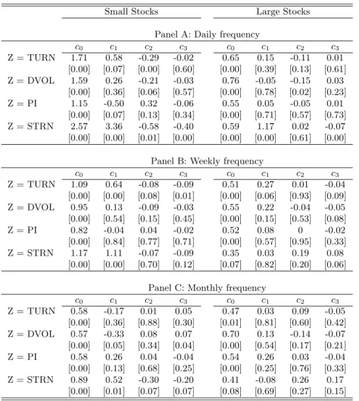
(18) To answer these criticisms, we estimate a parametric portfolio function. Given the smooth shapes observed in the nonparametric results, we postulate a polinomial shape for the optimal weight function: αsparam (Z) = c0 + c1 Z + c2 Z 2 + c3 Z 3. (10). The constants c0 ...c3 are estimated through GMM on the moment conditions T 1X mt+1 (αsparam (Zt )) ⊗ g(Zt ) = 0 T. (11). t=1. with g(Zt ) = [1, Zt , Zt2 , Zt3 ]. Note that the system is exactly identified. Significant c1 , c2 , or c3 parameters imply dependence of α on Z, i.e., a nonzero first derivative. The results in Table 8 show non-constant weights in broadly the same cases of the nonparametric method, and hence support our previous conclusions. One noteworthy finding in the monthly frequency is the statistical significance of the linear and cubic terms in the case of Dollar Volume for small stocks, implying a negative first derivative. As mentioned above, for Price Impact we do not find significance in any parameter (other than the constant c0 ) and hence cannot validate the nonparametric finding of a positive slope.. 5. Conclusion. This paper used a nonparametric technique to document the empirical relation between optimal portfolio weights for a CRRA investor and liquidity. Our main findings are the following. First, at very short horizons — daily and weekly — optimal stock allocations are strongly increasing functions of liquidity. This is consistent with increases in liquidity being followed by very short-term price increases, as documented in Gervais, Kaniel, and Mingelgrin (2001). These price increases are consistent with a decrease in the liquidity discount of Longstaff (2001). At longer monthly horizons, there is some evidence (though not very strong) of reversal of this relation, that is, optimal weights become decreasing functions of liquidity. This is consistent with increases in liquidity forecasting lower expected returns at the monthly or longer frequencies, as documented in Amihud (2002).. 16.

(19) Secondly, the three measures of liquidity tested do not produce the same results: the reversal mentioned above is visible in Dollar Volume, less so in Price Impact, and not so in Turnover. On the other hand, Turnover is a stronger determinant of optimal weights at shorter frequencies. Thirdly, the relation between liquidity and optimal weights is stronger for small than for large stocks. This inequality is consistent with most papers that have studied the relation between liquidity measures and expected returns. Fourthly, optimal weights for small stocks show a very strong dependence on Signed Turnover, which is consistent with the positive autocorrelation after high volume days found in Llorente, Michaely, Saar, and Wang (2000). Finally, the optimal portfolio functions are never negative, implying that short selling is not optimal for a CRRA investor that conditions his decisions on liquidity. This finding suggests that the low level of short selling observed in the US stock market may be simply due to the fact that it is not optimal to short sell. To summarize, our results suggest that in a real situation of portfolio management with rebalance at irregular, mixed frequencies, it may be fruitful to consider the information in the measures studied here for shorter-term trading decisions, while maintaining traditional predictors (dividend yield, term premium, default premium, etc.) for longer-term decisions.. 17.

(20) References A¨ıt-Sahalia, Yacine, and Michael W. Brandt, 2001, Variable selection for portfolio choice, Journal of Finance 56, 1297–1351. Almazan, Andres, Keith C. Brown, Murray Carlson, and David A. Chapman, 2002, Why constrain your mutual fund manager?, Working Paper, University of Texas at Austin. Amihud, Yakov, 2002, Illiquidity and stock returns: cross-section and time-series effects, Journal of Financial Markets 5, 31–56. Amihud, Yakov, and Haim Mendelson, 1986, Asset pricing and the bid-ask spread, Journal of Financial Economics 17, 223–249. Brandt, Michael W., 1999, Estimating portfolio and consumption choice: a conditional Euler equations approach, Journal of Finance 54, 1609–1646. Brennan, Michael J., Tarun Chordia, and Avanidhar Subrahmanyan, 1998, Alternative factor specifications, security characteristics, and the cross-section of expected stock returns, Journal of Financial Economics 49, 345–373. Brennan, Michael J., and Avanidhar Subrahmanyan, 1996, Market microstructure and asset pricing: on the compensation for illiquidity in stock returns, Journal of Financial Economics 41, 441–464. Campbell, John Y., Sanford J. Grossman, and Jiang Wang, 1993, Trading volume and serial correlation in stock returns, Quarterly Journal of Economics pp. 905–939. Chaudhuri, Probal, and J.S. Marron, 1999, SiZer for exploration of structures in curves, Journal of the American Statistical Association 94, 807–823. Conrad, Jennifer S., Allaudeen Hameed, and Cathy Niden, 1994, Volume and autocovariances in short-horizon individual security returns, Journal of Finance 49, 1305–1329. Datar, Vinay T., Narayan Y. Naik, and Robert Radcliffe, 1998, Liquidity and stock returns: An alternative test, Journal of Financial Markets 1, 203–219.. 18.

(21) D’Avolio, Gene, 2002, The market for borrowing stock, Journal of Financial Economics 66, 271–306. Eckbo, B. Espen, and Øyvind Norli, 2002, Pervasive liquidity risk, Working Paper, Dartmouth College. Geczy, Christopher C., David K. Musto, and Adam V. Reed, 2002, Stocks are special too: an analysis of the equity lending market, Journal of Financial Economics 66, 241–269. Gervais, Simon, Ron Kaniel, and Dan H. Mingelgrin, 2001, The high-volume return premium, Journal of Finance 56, 877–919. Horowitz, Joel L., 2000, The Bootstrap, Working Paper, University of Iowa. Inoue, Atsushi, and Mototsugu Shintani, 2001, Bootstrapping GMM Estimators for Time Series, Working Paper, North Carolina State University. Jones, Charles M., 2002, A century of stock market liquidity and trading costs, Working paper, Columbia University. LeBaron, Blake, 1992, Persistence of the Dow Jones index on rising volume, Working Paper, University of Wisconsin. Llorente, Guillermo, Roni Michaely, Gideon Saar, and Jiang Wang, 2000, Dynamic volumereturn relation of individual stocks, Working Paper, MIT. Lo, Andrew W., and Jiang Wang, 2000, Trading volume: definitions, data analysis, and implications of portfolio theory, Review of Financial Studies 13, 257–300. Longstaff, Francis A., 2001, Optimal portfolio choice and the valuation of illiquid securities, Review of Financial Studies 14, 407–431. Mehra, Rajnish, and Edward C. Prescott, 2003, The equity premium in retrospect, NBER Working Paper No. 9525. ˇ P´astor, Luboˇ s, and Robert F. Stambaugh, 2001, Liquidity risk and expected stock returns, NBER Working Paper No. 8462. 19.

(22) Politis, Dimitris N., and Joseph P. Romano, 1994, The stationary bootstrap, Journal of the American Statistical Association 89, 1303–13. Stickel, Scott E., and Robert E. Verrecchia, 1994, Evidence that trading volume sustains stock price changes, Financial Analysts Journal 50, 57–67. Sullivan, Ryan, Allan Timmermann, and Halbert White, 1999, Data-Snooping, Technical Trading Rule Performance, and the Bootstrap, Journal of Finance 54, 1647–1691.. 20.

(23) Table 1: Descriptive Statistics Descriptive statistics for daily values of the portfolio measures of liquidity. All variables are detrended and standardized, hence having a mean of 0 and a standard deviation of 1 by construction.. Mean Std Skewness Kurtosis. Small Stocks TURN DVOL 0.00 0.00 1.00 1.00 -0.16 -0.39 3.53 3.64. Percentiles: 5% -1.75 50% 0.01 95% 1.64. -1.84 0.05 1.55. Correlations: TURN 1.00 DVOL 0.90 PI -0.66 STRN 0.24 Rt+1 0.08. 1.00 -0.85 0.19 0.03. Portfolio PI STRN 0.00 0.00 1.00 1.00 0.84 -0.36 4.38 1.93. -1.43 -0.13 1.89. 1.00 -0.13 -0.01. Large Stocks TURN DVOL 0.00 0.00 1.00 1.00 0.46 -0.18 3.64 2.95. Portfolio PI STRN 0.00 0.00 1.00 1.00 0.61 -0.12 4.43 1.85. -1.53 0.45 1.29. -1.39 -0.14 1.84. -1.66 0.06 1.55. -1.54 -0.08 1.83. -1.47 0.51 1.38. 1.00 0.22. 1.00 0.68 -0.43 0.11 0.02. 1.00 -0.43 0.10 0.01. 1.00 -0.09 0.02. 1.00 0.10. 21.

(24) Table 2: Unconditional Portfolio Weights and Tests for Overidentifying Restrictions The investor allocates his wealth between a risk-free asset and either a portfolio of small stocks (columns under “Small Stocks”) or a portfolio of large stocks (columns under “Large Stocks”). In panel A, both the investment horizon and the rebalancing frequency are one day; in panel B, one week; and in C, one month. Each panel presents the unconditional allocation to the respective stock portfolio, obtained from equation (7). Standard-errors are in parenthesis. Each panel then also presents the test for overidentifying restrictions defined in equation (8), with p-values in square brackets. Each column corresponds to the following specification of instruments: g1 (Z) = [1, Z], g2 (Z) = [1, Z, Z 2 ], g3 (Z) = [1, Z, Z 2 , Z 3 ]. Small Stocks. Weight Test Overid Rest Z = TURN Z = DVOL Z = PI Z = STRN. Weight Test Overid Rest Z = TURN Z = DVOL Z = PI Z = STRN. Weight Test Overid Rest Z = TURN Z = DVOL Z = PI Z = STRN. Large Stocks. 1.29 (0.26) g1 (Z) 0.87 [0.35] 1.39 [0.24] 20.55 [0.00] 294.52 [0.00]. Panel A: Daily frequency 0.51 (0.13) g2 (Z) g3 (Z) g1 (Z) g2 (Z) 49.62 69.72 0.95 33.35 [0.00] [0.00] [0.33] [0.00] 12.38 18.70 1.96 37.23 [0.00] [0.00] [0.16] [0.00] 36.61 38.06 56.30 66.11 [0.00] [0.00] [0.00] [0.00] 297.27 372.70 242.34 245.52 [0.00] [0.00] [0.00] [0.00]. g3 (Z) 52.04 [0.00] 62.12 [0.00] 66.86 [0.00] 362.21 [0.00]. 0.84 (0.17) g1 (Z) 1.04 [0.31] 1.80 [0.18] 12.32 [0.00] 129.90 [0.00]. Panel B: Weekly frequency 0.50 (0.12) g2 (Z) g3 (Z) g1 (Z) g2 (Z) 25.49 35.53 1.05 8.38 [0.00] [0.00] [0.31] [0.02] 7.48 7.91 2.87 14.09 [0.02] [0.05] [0.09] [0.00] 16.24 18.03 19.29 24.72 [0.00] [0.00] [0.00] [0.00] 133.08 141.65 111.09 114.09 [0.00] [0.00] [0.00] [0.00]. g3 (Z) 14.69 [0.00] 20.00 [0.00] 27.23 [0.00] 135.74 [0.00]. 0.56 (0.10) g1 (Z) 1.39 [0.24] 1.49 [0.22] 4.90 [0.03] 57.18 [0.00]. Panel C: Monthly frequency 0.53 (0.13) g2 (Z) g3 (Z) g1 (Z) g2 (Z) 7.05 8.22 0.10 4.04 [0.03] [0.04] [0.76] [0.13] 2.08 3.26 0.61 5.55 [0.35] [0.35] [0.44] [0.06] 7.93 9.51 6.45 9.50 [0.02] [0.02] [0.01] [0.01] 57.86 61.58 46.21 46.68 [0.00] [0.00] [0.00] [0.00]. g3 (Z) 6.63 [0.08] 7.19 [0.07] 9.72 [0.02] 55.13 [0.00]. 22.

(25) Table 3: Optimal Portfolio Weights as a Function of Turnover The investor allocates his wealth between a risk-free asset and either a portfolio of small stocks (columns under “Small Stocks”) or a portfolio of large stocks (columns under “Large Stocks”). In panel A, both the investment horizon and the rebalancing frequency are one day; in panel B, one week; and in C, one month. Each panel presents the optimal allocation to the respective stock portfolio conditional on the value of Turnover indicated in the column heading. The optimal weight is the solution to equation (4). Standard-errors from the bootstrap detailed in section 4.2 are in parenthesis. The slope at each value of the predictor variable is obtained from equation (9). Bootstrap t-statistics for a zero slope are in curly braces.. Small Stocks. Weight Slope. Weight Slope. Weight Slope. Large Stocks. Z=-2 0.72 (0.24) 0.48 {4.90}. Z=-1 1.18 (0.22) 0.42 {4.56}. Z=0 1.52 (0.22) 0.24 {1.88}. Z=1 1.64 (0.30) 0.01 {0.09}. Panel A: Daily Z=2 1.58 (0.45) -0.13 {-0.68}. frequency Z=-2 Z=-1 0.41 0.52 (0.16) (0.14) 0.13 0.1 {2.26} {2.16}. Z=0 0.6 (0.13) 0.07 {1.54}. Z=1 0.65 (0.13) 0.02 {0.26}. Z=2 0.62 (0.16) -0.1 {-0.92}. Z=-2 0.59 (0.17) 0.16 {2.15}. Z=-1 0.76 (0.17) 0.18 {2.85}. Z=0 0.93 (0.17) 0.16 {2.96}. Panel B: Weekly frequency Z=1 Z=2 Z=-2 Z=-1 1.07 1.07 0.37 0.43 (0.19) (0.25) (0.14) (0.13) 0.09 -0.11 0.05 0.08 {1.37} {-0.79} {0.89} {1.77}. Z=0 0.52 (0.13) 0.08 {1.59}. Z=1 0.59 (0.14) 0.05 {0.84}. Z=2 0.62 (0.17) 0.02 {0.25}. Z=-2 0.61 (0.18) 0.05 {0.30}. Z=-1 0.6 (0.13) -0.05 {-0.52}. Z=0 0.55 (0.13) -0.02 {-0.29}. Panel C: Monthly frequency Z=1 Z=2 Z=-2 Z=-1 0.56 0.55 0.61 0.57 (0.15) (0.23) (0.24) (0.16) 0.01 -0.02 -0.01 -0.06 {0.10} {-0.15} {-0.07} {-0.57}. Z=0 0.5 (0.14) -0.07 {-0.69}. Z=1 0.48 (0.15) 0.04 {0.27}. Z=2 0.55 (0.30) 0.05 {0.19}. 23.

(26) Table 4: Optimal Portfolio Weights as a Function of Dollar Volume The investor allocates his wealth between a risk-free asset and either a portfolio of small stocks (columns under “Small Stocks”) or a portfolio of large stocks (columns under “Large Stocks”). In panel A, both the investment horizon and the rebalancing frequency are one day; in panel B, one week; and in C, one month. Each panel presents the optimal allocation to the respective stock portfolio conditional on the value of Dollar Volume indicated in the column heading. The optimal weight is the solution to equation (4). Standard-errors from the bootstrap detailed in section 4.2 are in parenthesis. The slope at each value of the predictor variable is obtained from equation (9). Bootstrap t-statistics for a zero slope are in curly braces.. Small Stocks. Weight Slope. Weight Slope. Weight Slope. Large Stocks. Z=-2 1.05 (0.23) 0.28 {2.62}. Z=-1 1.29 (0.21) 0.19 {2.06}. Z=0 1.43 (0.23) 0.08 {0.68}. Panel A: Daily Z=1 Z=2 1.45 1.41 (0.29) (0.40) -0.02 -0.06 {-0.15} {-0.43}. frequency Z=-2 Z=-1 0.49 0.59 (0.17) (0.14) 0.14 0.07 {1.93} {1.30}. Z=0 0.64 (0.13) 0.01 {0.21}. Z=1 0.61 (0.14) -0.06 {-0.92}. Z=2 0.52 (0.17) -0.13 {-1.48}. Z=-2 0.78 (0.17) 0.08 {0.91}. Z=-1 0.85 (0.16) 0.06 {0.85}. Z=0 0.89 (0.17) 0.02 {0.38}. Panel B: Weekly frequency Z=1 Z=2 Z=-2 Z=-1 0.89 0.85 0.41 0.48 (0.20) (0.25) (0.15) (0.13) -0.02 -0.06 0.07 0.07 {-0.29} {-0.67} {1.04} {1.24}. Z=0 0.54 (0.13) 0.03 {0.61}. Z=1 0.56 (0.14) 0 {0.08}. Z=2 0.55 (0.16) -0.01 {-0.14}. Z=-2 0.82 (0.18) -0.04 {-0.21}. Z=-1 0.68 (0.13) -0.16 {-1.70}. Z=0 0.55 (0.12) -0.1 {-1.24}. Panel C: Monthly frequency Z=1 Z=2 Z=-2 Z=-1 0.47 0.45 0.5 0.62 (0.15) (0.19) (0.25) (0.16) -0.06 0.03 0.13 0.06 {-0.72} {0.25} {0.72} {0.40}. Z=0 0.61 (0.14) -0.05 {-0.51}. Z=1 0.54 (0.15) -0.1 {-0.78}. Z=2 0.39 (0.25) -0.21 {-1.02}. 24.

(27) Table 5: Optimal Portfolio Weights as a Function of Price Impact The investor allocates his wealth between a risk-free asset and either a portfolio of small stocks (columns under “Small Stocks”) or a portfolio of large stocks (columns under “Large Stocks”). In panel A, both the investment horizon and the rebalancing frequency are one day; in panel B, one week; and in C, one month. Each panel presents the optimal allocation to the respective stock portfolio conditional on the value of Price Impact indicated in the column heading. The optimal weight is the solution to equation (4). Standard-errors from the bootstrap detailed in section 4.2 are in parenthesis. The slope at each value of the predictor variable is obtained from equation (9). Bootstrap t-statistics for a zero slope are in curly braces.. Small Stocks. Weight Slope. Weight Slope. Weight Slope. Large Stocks. Z=-2 1.54 (0.32) -0.15 {-2.37}. Z=-1 1.4 (0.29) -0.13 {-2.10}. Z=0 1.29 (0.27) -0.1 {-1.59}. Panel A: Daily frequency Z=1 Z=2 Z=-2 Z=-1 1.19 1.09 0.45 0.48 (0.25) (0.25) (0.18) (0.16) -0.1 -0.11 0.02 0.04 {-1.18} {-0.99} {0.40} {0.78}. Z=0 0.52 (0.14) 0.04 {0.99}. Z=1 0.56 (0.14) 0.03 {0.59}. Z=2 0.57 (0.14) -0.02 {-0.21}. Z=-2 0.88 (0.25) -0.03 {-0.51}. Z=-1 0.86 (0.22) -0.02 {-0.37}. Z=0 0.84 (0.19) -0.01 {-0.17}. Panel B: Weekly Z=1 Z=2 0.83 0.81 (0.17) (0.18) -0.01 -0.05 {-0.18} {-0.51}. frequency Z=-2 Z=-1 0.5 0.52 (0.17) (0.14) 0.01 0.02 {0.18} {0.37}. Z=0 0.54 (0.13) 0.01 {0.18}. Z=1 0.53 (0.13) -0.02 {-0.36}. Z=2 0.49 (0.14) -0.07 {-0.82}. Z=-2 0.45 (0.19) -0.01 {-0.06}. Z=-1 0.47 (0.15) 0.06 {0.78}. Z=0 0.56 (0.13) 0.11 {1.36}. Panel C: Monthly frequency Z=1 Z=2 Z=-2 Z=-1 0.68 0.76 0.39 0.43 (0.13) (0.20) (0.28) (0.16) 0.11 0.06 0.02 0.07 {1.00} {0.31} {0.07} {0.50}. Z=0 0.52 (0.14) 0.12 {1.31}. Z=1 0.7 (0.15) 0.23 {1.65}. Z=2 0.8 (0.28) -0.18 {-0.59}. 25.

(28) Table 6: Optimal Portfolio Weights as a Function of Signed Turnover The investor allocates his wealth between a risk-free asset and either a portfolio of small stocks (columns under “Small Stocks”) or a portfolio of large stocks (columns under “Large Stocks”). In panel A, both the investment horizon and the rebalancing frequency are one day; in panel B, one week; and in C, one month. Each panel presents the optimal allocation to the respective stock portfolio conditional on the value of Signed Turnover indicated in the column heading. The optimal weight is the solution to equation (4). Standard-errors from the bootstrap detailed in section 4.2 are in parenthesis. The slope at each value of the predictor variable is obtained from equation (9). Bootstrap t-statistics for a zero slope are in curly braces. Small Stocks. Weight Slope. Weight Slope. Weight Slope. Large Stocks. Z=-2 -0.66 (0.20) 0.67 {7.46}. Z=-1 0.31 (0.22) 1.21 {15.64}. Z=0 1.59 (0.24) 1.27 {10.38}. Panel A: Daily frequency Z=1 Z=2 Z=-2 Z=-1 2.71 3.47 -0.34 0.04 (0.31) (0.41) (0.14) (0.14) 0.93 0.6 0.25 0.49 {5.86} {4.08} {5.64} {9.71}. Z=0 0.61 (0.14) 0.61 {9.39}. Z=1 1.17 (0.16) 0.47 {6.08}. Z=2 1.49 (0.20) 0.19 {2.71}. Z=-2 0.18 (0.15) 0.26 {5.74}. Z=-1 0.52 (0.16) 0.42 {7.38}. Z=0 0.98 (0.17) 0.47 {6.76}. Panel B: Weekly frequency Z=1 Z=2 Z=-2 Z=-1 1.41 1.71 0.45 0.46 (0.19) (0.22) (0.15) (0.13) 0.37 0.24 0.01 0.02 {4.94} {3.23} {0.15} {0.33}. Z=0 0.49 (0.12) 0.05 {0.76}. Z=1 0.55 (0.14) 0.06 {1.28}. Z=2 0.62 (0.16) 0.06 {1.37}. Z=-2 0.22 (0.14) 0.08 {2.07}. Z=-1 0.4 (0.13) 0.29 {4.05}. Z=0 0.71 (0.13) 0.26 {2.15}. Panel C: Monthly Z=1 Z=2 0.83 0.78 (0.19) (0.26) 0.00 -0.07 {-0.03} {-0.83}. Z=0 0.56 (0.14) 0.05 {0.48}. Z=1 0.6 (0.16) 0.04 {0.64}. Z=2 0.65 (0.19) 0.07 {1.10}. 26. frequency Z=-2 Z=-1 0.45 0.51 (0.21) (0.16) 0.06 0.05 {0.58} {0.54}.

(29) Table 7: Optimal Portfolio Weights as a Function of Price Impact for Different Degrees of Risk Aversion The investor allocates his wealth between a risk-free asset and either a portfolio of small stocks (columns under “Small Stocks”) or a portfolio of large stocks (columns under “Large Stocks”). In panel A, both the investment horizon and the rebalancing frequency are one day; in panel B, one week; and in C, one month. Each panel presents the optimal allocation to the respective stock portfolio conditional on the value of Price Impact indicated in the column heading. The optimal weight is the solution to equation (4). The coefficient γ defines the degree of risk aversion of the CRRA utility function in equation (2). Small Stocks. γ γ γ γ. γ γ γ γ. γ γ γ γ. Large Stocks. =3 =5 = 10 = 20. Z=-2 4.50 2.93 1.54 0.79. Z=-1 4.20 2.70 1.40 0.71. Z=0 3.96 2.50 1.29 0.65. Panel A: Daily Z=1 Z=2 3.74 3.51 2.33 2.15 1.19 1.09 0.60 0.55. frequency Z=-2 Z=-1 1.47 1.56 0.89 0.95 0.45 0.48 0.23 0.24. Z=0 1.69 1.03 0.52 0.26. Z=1 1.82 1.11 0.56 0.28. Z=2 1.87 1.13 0.57 0.29. =3 =5 = 10 = 20. Z=-2 2.71 1.71 0.88 0.45. Z=-1 2.65 1.67 0.86 0.43. Z=0 2.64 1.65 0.84 0.43. Panel B: Weekly frequency Z=1 Z=2 Z=-2 Z=-1 2.65 2.62 1.64 1.72 1.64 1.60 0.99 1.04 0.83 0.81 0.50 0.52 0.42 0.40 0.25 0.26. Z=0 1.78 1.07 0.54 0.27. Z=1 1.77 1.06 0.53 0.27. Z=2 1.63 0.98 0.49 0.25. =3 =5 = 10 = 20. Z=-2 1.40 0.87 0.45 0.23. Z=-1 1.46 0.92 0.47 0.24. Z=0 1.72 1.09 0.56 0.28. Panel Z=1 2.09 1.32 0.68 0.34. Z=0 1.71 1.04 0.52 0.26. Z=1 2.30 1.40 0.70 0.35. Z=2 2.62 1.59 0.80 0.40. C: Monthly frequency Z=2 Z=-2 Z=-1 2.46 1.25 1.42 1.52 0.77 0.86 0.76 0.39 0.43 0.38 0.20 0.22. 27.

(30) Table 8: Parametric Estimators of Conditional Portfolio Weights The investor allocates his wealth between a risk-free asset and either a portfolio of small stocks (columns under “Small Stocks”) or a portfolio of large stocks (columns under “Large Stocks”). In panel A, both the investment horizon and the rebalancing frequency are one day; in panel B, one week; and in C, one month. Each panel gives estimates of the parameters ci for the optimal portfolio function defined in equation (10). These estimates are obtained through GMM on the moment conditions (11). P-values are in square brackets. Small Stocks. Z = TURN Z = DVOL Z = PI Z = STRN. Z = TURN Z = DVOL Z = PI Z = STRN. Z = TURN Z = DVOL Z = PI Z = STRN. Large Stocks. c0 1.71 [0.00] 1.59 [0.00] 1.15 [0.00] 2.57 [0.00]. c1 0.58 [0.07] 0.26 [0.36] -0.50 [0.07] 3.36 [0.00]. Panel A: Daily c2 c3 -0.29 -0.02 [0.00] [0.60] -0.21 -0.03 [0.06] [0.57] 0.32 -0.06 [0.13] [0.34] -0.58 -0.40 [0.01] [0.00]. frequency c0 c1 0.65 0.15 [0.00] [0.39] 0.76 -0.05 [0.00] [0.78] 0.55 0.05 [0.00] [0.71] 0.59 1.17 [0.00] [0.00]. c2 -0.11 [0.13] -0.15 [0.02] -0.05 [0.57] 0.02 [0.61]. c3 0.01 [0.61] 0.03 [0.23] 0.01 [0.73] -0.07 [0.00]. c0 1.09 [0.00] 0.95 [0.00] 0.82 [0.00] 1.17 [0.00]. c1 0.64 [0.00] 0.13 [0.54] -0.04 [0.84] 1.11 [0.00]. Panel B: Weekly frequency c2 c3 c0 c1 -0.08 -0.09 0.51 0.27 [0.08] [0.01] [0.00] [0.06] -0.09 -0.03 0.55 0.22 [0.15] [0.45] [0.00] [0.15] 0.04 -0.02 0.52 0.08 [0.77] [0.71] [0.00] [0.57] -0.07 -0.09 0.35 0.03 [0.70] [0.12] [0.07] [0.82]. c2 0.01 [0.93] -0.04 [0.53] 0 [0.95] 0.19 [0.20]. c3 -0.04 [0.09] -0.05 [0.08] -0.02 [0.33] 0.08 [0.06]. c0 0.58 [0.00] 0.57 [0.00] 0.58 [0.00] 0.89 [0.00]. c1 -0.17 [0.36] -0.33 [0.05] 0.26 [0.13] 0.52 [0.01]. Panel C: Monthly frequency c2 c3 c0 c1 0.01 0.05 0.47 0.03 [0.88] [0.30] [0.01] [0.81] 0.08 0.07 0.70 0.13 [0.34] [0.04] [0.00] [0.54] 0.04 -0.04 0.54 0.26 [0.68] [0.25] [0.00] [0.25] -0.30 -0.20 0.41 -0.08 [0.07] [0.07] [0.08] [0.69]. c2 0.09 [0.60] -0.14 [0.17] 0.03 [0.76] 0.26 [0.27]. c3 -0.05 [0.42] -0.07 [0.21] -0.04 [0.33] 0.17 [0.15]. 28.

(31) Figure 1: Time Series of Raw Data Each plot displays raw (before detrending) monthly data for the indicated liquidity measure. The bold line in each panel represents the portfolio of large stocks (deciles 9 and 10 of the NYSE); the thinner line represents the portfolio of small stocks (deciles 2 and 3 of the NYSE).. 0.1. 0.05. 0 1960. 1965. 1970. 1975. 1980. 1985. 1990. 1995. 2000. 2005. 1990. 1995. 2000. 2005. 1990. 1995. 2000. 2005. Dollar Volume. 11. x 10 12 10. Dollars. 8 6 4 2 0 1960. 1965. 1970. 1975. 1980. 1985. Price Impact. −6. x 10 7 6 5. |R|/DVOL. Prop Shrs Outstd. Turnover. 4 3 2 1 0 1960. 1965. 1970. 1975. 1980. 29. 1985.

(32) Figure 2: Optimal Portfolio Weights as a Function of Turnover The investor allocates his wealth between a risk-free asset and either a portfolio of small stocks (left column) or a portfolio of large stocks (right column). In the first row, both the investment horizon and the rebalancing frequency are one day; in the second row, one week; and in the third, one month. The bold line in each panel represents the optimal fraction of wealth allocated to the respective stock portfolio as a function of Turnover. Each point in this function is the solution to equation (4). The thin horizontal line represents the optimal unconditional allocation, which is given by equation (7). Large stocks, Daily 2. 1.5. 1.5. Portfolio weight. Portfolio weight. Small stocks, Daily 2. 1. 0.5. 0 −2. 1. 0.5. −1. 0 TURN. 1. 0 −2. 2. 2. 1.5. 1.5. 1. 0.5. 0 −2. 2. 0.5. −1. 0 TURN. 1. 0 −2. 2. Small stocks, Monthly. −1. 0 TURN. 1. 2. Large stocks, Monthly 2. 1.5. 1.5. Portfolio weight. Portfolio weight. 1. 1. 2. 1. 0.5. 0 −2. 0 TURN. Large stocks, Weekly. 2. Portfolio weight. Portfolio weight. Small stocks, Weekly. −1. 1. 0.5. −1. 0 TURN. 1. 0 −2. 2. 30. −1. 0 TURN. 1. 2.

(33) Figure 3: Optimal Portfolio Weights as a Function of Dollar Volume The investor allocates his wealth between a risk-free asset and either a portfolio of small stocks (left column) or a portfolio of large stocks (right column). In the first row, both the investment horizon and the rebalancing frequency are one day; in the second row, one week; and in the third, one month. The bold line in each panel represents the optimal fraction of wealth allocated to the respective stock portfolio as a function of Dollar Volume. Each point in this function is the solution to equation (4). The thin horizontal line represents the optimal unconditional allocation, which is given by equation (7). Large stocks, Daily 2. 1.5. 1.5. Portfolio weight. Portfolio weight. Small stocks, Daily 2. 1. 0.5. 0 −2. 1. 0.5. −1. 0 DVOL. 1. 0 −2. 2. 2. 1.5. 1.5. 1. 0.5. 0 −2. 2. 0.5. −1. 0 DVOL. 1. 0 −2. 2. Small stocks, Monthly. −1. 0 DVOL. 1. 2. Large stocks, Monthly 2. 1.5. 1.5. Portfolio weight. Portfolio weight. 1. 1. 2. 1. 0.5. 0 −2. 0 DVOL. Large stocks, Weekly. 2. Portfolio weight. Portfolio weight. Small stocks, Weekly. −1. 1. 0.5. −1. 0 DVOL. 1. 0 −2. 2. 31. −1. 0 DVOL. 1. 2.

(34) Figure 4: Optimal Portfolio Weights as a Function of Price Impact The investor allocates his wealth between a risk-free asset and either a portfolio of small stocks (left column) or a portfolio of large stocks (right column). In the first row, both the investment horizon and the rebalancing frequency are one day; in the second row, one week; and in the third, one month. The bold line in each panel represents the optimal fraction of wealth allocated to the respective stock portfolio as a function of Price Impact. Each point in this function is the solution to equation (4). The thin horizontal line represents the optimal unconditional allocation, which is given by equation (7). Large stocks, Daily 2. 1.5. 1.5. Portfolio weight. Portfolio weight. Small stocks, Daily 2. 1. 0.5. 0 −2. 1. 0.5. −1. 0 PI. 1. 0 −2. 2. 2. 1.5. 1.5. 1. 0.5. 0 −2. 2. 0.5. −1. 0 PI. 1. 0 −2. 2. Small stocks, Monthly. −1. 0 PI. 1. 2. Large stocks, Monthly 2. 1.5. 1.5. Portfolio weight. Portfolio weight. 1. 1. 2. 1. 0.5. 0 −2. 0 PI. Large stocks, Weekly. 2. Portfolio weight. Portfolio weight. Small stocks, Weekly. −1. 1. 0.5. −1. 0 PI. 1. 0 −2. 2. 32. −1. 0 PI. 1. 2.

(35) Figure 5: Optimal Portfolio Weights as a Function of Signed Turnover The investor allocates his wealth between a risk-free asset and either a portfolio of small stocks (left column) or a portfolio of large stocks (right column). In the first row, both the investment horizon and the rebalancing frequency are one day; in the second row, one week; and in the third, one month. The bold line in each panel represents the optimal fraction of wealth allocated to the respective stock portfolio as a function of Signed Turnover. Each point in this function is the solution to equation (4). The thin horizontal line represents the optimal unconditional allocation, which is given by equation (7). Large stocks, Daily 3. 2.5. 2.5. 2. 2. Portfolio weight. Portfolio weight. Small stocks, Daily 3. 1.5 1 0.5 0 −0.5 −2. 1.5 1 0.5 0. −1. 0 STRN. 1. −0.5 −2. 2. 3. 2.5. 2.5. 2. 2. 1.5 1 0.5 0 −0.5 −2. 2. 1 0.5 0. −1. 0 STRN. 1. −0.5 −2. 2. Small stocks, Monthly. −1. 0 STRN. 1. 2. Large stocks, Monthly 3. 2.5. 2.5. 2. 2. Portfolio weight. Portfolio weight. 1. 1.5. 3. 1.5 1 0.5 0 −0.5 −2. 0 STRN. Large stocks, Weekly. 3. Portfolio weight. Portfolio weight. Small stocks, Weekly. −1. 1.5 1 0.5 0. −1. 0 STRN. 1. −0.5 −2. 2. 33. −1. 0 STRN. 1. 2.

(36)