The Economy-wide Impacts of the South African Child Support Grant: a Micro-Simulation-Computable General Equilibrium Analysis

Tiberti : Université Laval, CIRPÉE and PEP network, Canada Maisonnave : Université Laval, CIRPÉE and PEP network, Canada

Chitiga : (Corresponding author) Human Science Research Council, Private Bag X41, Pretoria, 0001, South Africa.

Tel.: +27 12 302 2406 MChitiga@hsrc.ac.za

Mabugu : Financial and Fiscal Commission, South Africa Robichaud : Human Science Research Council, South Africa Ngandu : Human Science Research Council, South Africa

Cahier de recherche/Working Paper 13-03

The Economy-wide Impacts of the South African Child Support Grant :

a Micro-Simulation-Computable General Equilibrium Analysis

Luca Tiberti

Hélène Maisonnave

Margaret Chitiga

Ramos Mabugu

Véronique Robichaud

Stewart Ngandu

Mars/March 2013

Abstract:

We examine the economy-wide impact of the child support grant (CSG) on the South

African economy using a bottom-up/top-down approach. This allows us to estimate the

potential effects on households’ welfare and on the economy following a change in the

CSG. Three simulations are presented, in simulation 1 the value of the CSG is increased

by 20%; in simulation 2 the number of beneficiaries among the eligible children is

increased by two million and simulation 3 combines these two. A positive link between

the CSG and the probability of participating in the labour market is found. The positive

impacts on the labour market, together with the increase in the transfers received by

households, results in an increase in their income. Poverty decreases in comparison

with the base year for the whole population and for children. Finally, we can conclude

that simulation 1 is the most cost effective of the policies.

Keywords: Child support grant, computable general equilibrium, micro-simulation,

poverty, South Africa

1 I

NTRODUCTION

The South African Child Support Grant (CSG) was introduced in April 1998 where it replaced the child maintenance grant. The adoption of the CSG contributed to South Africa’s progressive realisation of the constitutional right to social security as enshrined in article 27 of the Republic of South Africa Constitution (1996). The grant, which is paid to the child’s primary caregiver, is currently the most important form of assistance for children in poor families and offers a potential source of protection against poverty. The CSG has expanded markedly in recent years, until 2008, it was only available to children aged 0-13 years, in 2009, this was extended to include children aged 14 and from 2010 the age of eligibility was increased to include children up to the age of 18 years (South Africa Social Security Agency (SASSA), 2010). Since 1 April 2012, the CSG amounts to R280 per month, with an estimated 10 977 000 beneficiaries as of 31 March 2011 (National Treasury, 2011). Given the importance and scale of the CSG, this study assesses the economy-wide impact of changes in the scheme based on two potential policy changes as well as their combined effect. Firstly, as will be discussed in section 2.1, the number of beneficiaries is likely to increase by 2 million over the next few years. Secondly, the value of the grant itself is also expected to rise over the same period (see section 2.2). Both these two developments will have an impact on the South African economy especially as it relates to changes in poverty severity, incidence and depth. This paper is structured as follows: Section 2 discusses the CSG in South Africa, looking at coverage in terms of the number of beneficiaries and changes in eligibility over the years. Section 3 briefly reviews literature on the impact of social transfer programmes, while section 4 discusses the methodology and data used for this study. Section 5 discusses the results of the 3 simulations carried out based on the potential changes in the welfare scheme, and then section 6 concludes the paper.

2 O

VERVIEW OF

S

OUTH

A

FRICA

’

S

C

HILD

S

UPPORT

G

RANT

This section gives a brief overview of South Africa’s CSG. It focuses on its reach, expenditure and the impact it has had on both poverty and the lives of grant recipients.

2.1 Reach of the CSG

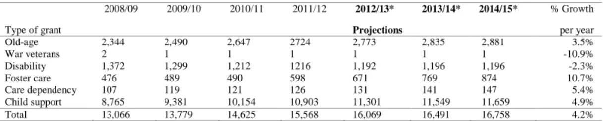
At the time of its introduction, the declared goal was for the CSG to reach 3 million children within 5 years. Fourteen years later the CSG has expanded rapidly with over 10 million beneficiaries, making it the largest social assistance programme in South Africa and one of the largest globally. Table 1 shows changes in social grant beneficiaries by type from 2008 with projections to 2015. From the table, it is clear that the CSG has the highest number of beneficiaries growing at 4.9% over the reported period.

Table 1: Social grants beneficiary numbers by type and province, 2008/07 – 2014/15 in 000's

2008/09 2009/10 2010/11 2011/12 2012/13* 2013/14* 2014/15* % Growth

Type of grant Projections per year

Old-age 2,344 2,490 2,647 2724 2,773 2,835 2,881 3.5% War veterans 2 1 1 1 1 1 1 -10.9% Disability 1,372 1,299 1,212 1216 1,192 1,196 1,196 -2.3% Foster care 476 489 490 598 671 769 874 10.7% Care dependency 107 119 121 126 131 141 147 5.4% Child support 8,765 9,381 10,154 10,903 11,301 11,549 11,659 4.9% Total 13,066 13,779 14,625 15,568 16,069 16,491 16,758 4.2%

Source: National Budget Review (2012) * Projected numbers at fiscal year-end.

This growth has continued despite many initial challenges with the implementation of the CSG. These included the lack of equipment in many offices, under staffing of welfare offices, lack of uniformity in the application process across provinces and offices, problems with accessing vital registration documents (for example, identity documents and birth certificates) and difficulties in providing postal addresses (Eyal et al, 2011).

Although the number of beneficiaries has increased over the years, there is evidence that a significant number of eligible children are not able to access the grant. More than 600,000 maternal orphans are not receiving any grant, a vastly higher proportion than for any other group (Southern Africa Labour and Development Research Unit’s National Income Dynamics Study, 2008). In addition, disproportionately fewer younger children (0-2 years) as well as fewer rural children are accessing the CSG (McEwan et al, 2010). The Department of Social Development acknowledges that not all children eligible for the CSG are receiving it, citing lack of documentation as the biggest barrier alongside some of the challenges mentioned above. According to SASSA (2010), in 2008, 2.1 million children or 27% of those eligible for the CSG did not receive it.

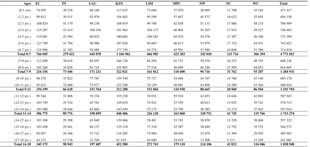
At the regional level, Table 2 indicates that KwaZulu-Natal and Eastern Cape have the highest number of children who are benefiting from the CSG with children under 7 years being the largest age group of CSG beneficiaries. The figures for these two largely rural provinces in particular demonstrate the ability of the CSG to reach large numbers of poor children, including those living in deep rural areas.

Table 2: Number of Child Support Grants by age and province as at 30 June 2011

Ages EC FS GAU KZN LIM MPU NW NC WC Total

(0-1 yrs) 74 455 30 236 66 160 113 815 73 040 37 870 28 969 11 708 35 164 471 417 (1-2 yrs ) 99 812 39 511 92 978 156 402 95 599 57 607 45 572 16 622 52 055 656 158 (2-3 yrs ) 108 824 41 170 98 238 168 819 99 788 62 838 51 131 17 886 58 215 706 909 (3-4 yrs ) 119 287 43 414 100 194 181 963 104 137 66 804 54 203 17 933 58 527 746 462 (4-5 yrs ) 119 881 41 994 96 833 180 604 100 542 65 476 54 576 17 387 56 106 733 399 (5-6 yrs ) 123 790 41 794 96 986 187 620 99 603 66 617 53 979 17 332 54 931 742 652 (6-7 yrs ) 119 996 41 303 93 689 177 739 94 276 65 991 53 580 16 848 51 396 714 818 Total 0-7 766 045 279 422 645 078 1 166 962 666 985 423 203 342 010 115 716 366 394 4 771 815 (7-8 yrs ) 112 890 38 618 89 497 166 128 84 294 61 731 50 470 16 253 48 355 668 236 (8-9 yrs ) 103 266 34 828 81 714 155 893 77 518 56 869 46 246 15 509 44 852 616 695 Total 7-9 216 156 73 446 171 211 322 021 161 812 118 600 96 716 31 762 93 207 1 284 931 (9-10 yrs ) 98 578 33 822 77 787 159 740 75 727 54 849 44 767 14 760 43 140 603 170 (10-11 yrs ) 95 621 32 806 73 977 152 548 76 129 56 081 43 898 14 200 43 364 588 624 Total 9-11 194 199 66 628 151 764 312 288 151 856 110 930 88 665 28 960 86 504 1 191 794 (11-12 yrs ) 99 546 31 806 70 234 155 238 76 031 55 910 42 453 14 646 42 083 587 947 (12-13 yrs ) 103 749 29 324 65 761 149 619 74 922 53 359 40 013 13 825 39 741 570 313 (13-14 yrs ) 103 480 28 646 62 864 143 549 75 175 53 799 38 285 13 274 37 942 557 014 Total 11-14 306 775 89 776 198 859 448 406 226 128 163 068 120 751 41 745 119 766 1 715 274 (14-15 yrs ) 103 388 29 398 63 840 139 666 76 481 53 763 38 870 13 320 38 606 557 332 (15-16 yrs ) 103 458 29 461 60 137 135 218 77 318 52 387 38 049 12 792 35 752 544 572 (16-17 yrs ) 94 057 26 366 51 721 116 285 74 904 48 049 33 679 11 399 29 503 485 963 (17-18 yrs ) 44 272 13 718 21 709 61 419 44 040 24 919 13 508 5 311 12 185 241 081 Total 14-18 345 175 98 943 197 407 452 588 272 743 179 118 124 106 42 822 116 046 1 828 948 Key: EC – Eastern Cape; FS – Free State; GAU – Gauteng; KZN – KwaZulu Natal; Lim – Limpopo; MPU – Mpumalanga; NW –NorthWest; NC – Northern Cape; WC – Western Cape Source: South African Social Security Agency Third Quarter Indicator Report December 2011

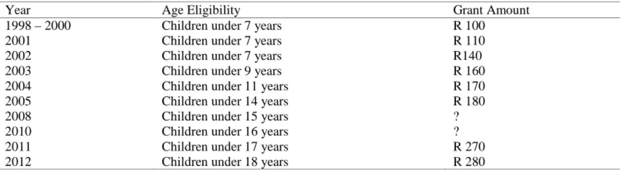
Table 3: Changes in Age Eligibility and Grant Value Progression of the CSG

Year Age Eligibility Grant Amount

1998 – 2000 Children under 7 years R 100

2001 Children under 7 years R 110

2002 Children under 7 years R140

2003 Children under 9 years R 160

2004 Children under 11 years R 170

2005 Children under 14 years R 180

2008 Children under 15 years ?

2010 Children under 16 years ?

2011 Children under 17 years R 270

2012 Children under 18 years R 280

Source: Eyal et al (2011)

As Table 3 indicates, both the age of eligibility and the value of the CSG have increased gradually over time from covering children less than 7 years (1998-2000), to covering children less than 18 years in 2012 and from a grant amount of R100 to its current value of R280 per month. The “follow the child” concept adopted for the implementation of the CSG is unique in that it recognized the varied and fluid nature of the family structure in South Africa and instead of linking the grant to a biological parent it allows the grant to be accessed by a primary caregiver. The primary caregiver is defined as anyone older than 16 years who is taking primary responsibility for the day to day needs of that child whether parent, relative or unrelated carer (Patel et al, 2012).

2.2 Spending on CSG

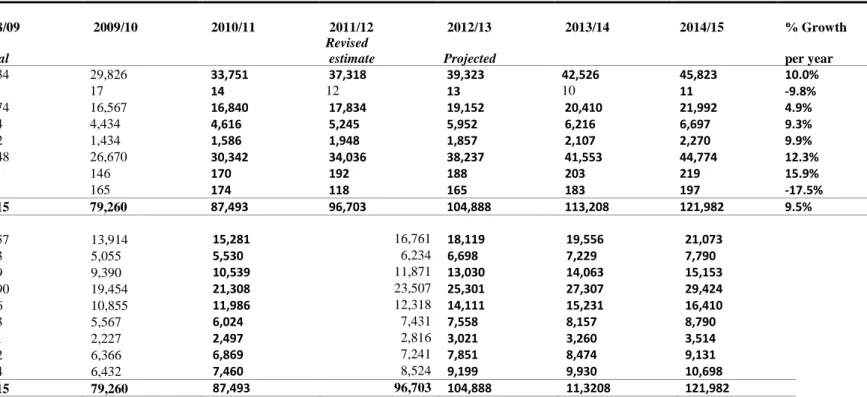
In the 2011/12 fiscal year, spending on social assistance in South Africa was R96,203 billion with a significant amount of that going towards the cost of the CSG as seen in Table 4 which shows social grants expenditure by type and province. It is the size of the CSG expenditure in South Africa’s social spending that forms part of the motivation for this paper. All in all, expenditure on social assistance represents approximately 3.5% of Gross Domestic Product

Table 4: Social grants expenditure by type and province, 2007/08– 2013/14

2008/09 2009/10 2010/11 2011/12 2012/13 2013/14 2014/15 % Growth

R million Actual

Revised

estimate Projected per year

Old-age 25,934 29,826 33,751 37,318 39,323 42,526 45,823 10.0% War veterans 20 17 14 12 13 10 11 -9.8% Disability 16,474 16,567 16,840 17,834 19,152 20,410 21,992 4.9% Foster care 3,934 4,434 4,616 5,245 5,952 6,216 6,697 9.3% Care dependency 1,292 1,434 1,586 1,948 1,857 2,107 2,270 9.9% Child support 22,348 26,670 30,342 34,036 38,237 41,553 44,774 12.3% Grant-in-aid 90 146 170 192 188 203 219 15.9%

Social relief of distress 623 165 174 118 165 183 197 -17.5%

Total 70,715 79,260 87,493 96,703 104,888 113,208 121,982 9.5% Province Eastern Cape 12,557 13,914 15,281 16,761 18,119 19,556 21,073 Free State 4,573 5,055 5,530 6,234 6,698 7,229 7,790 Gauteng 8,289 9,390 10,539 11,871 13,030 14,063 15,153 Kw aZulu-Natal 17,590 19,454 21,308 23,507 25,301 27,307 29,424 Limpopo 9,656 10,855 11,986 12,318 14,111 15,231 16,410 Mpumalanga 4,943 5,567 6,024 7,431 7,558 8,157 8,790 Northern Cape 5,711 2,227 2,497 2,816 3,021 3,260 3,514 North West 1,962 6,366 6,869 7,241 7,851 8,474 9,131 Western Cape 5,434 6,432 7,460 8,524 9,199 9,930 10,698 Total 70,715 79,260 87,493 96,703 104,888 11,3208 121,982

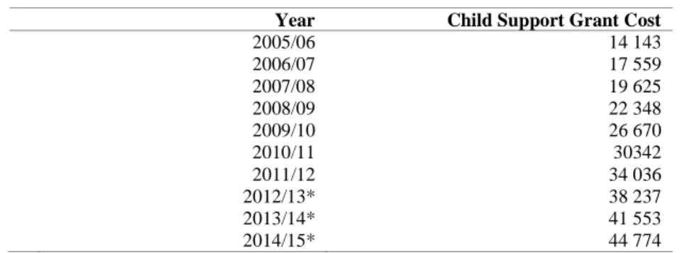
Seeking (2007) argues that this is unique in that no other developing country redistributes as large a share of its GDP through social assistance programmes as South Africa is doing. More importantly, according to National Treasury (2011) projections, these costs are going to continue rising as the size and cost of the CSG is driven in the main by the progressive increases in the age limit and the means test threshold adjustments as seen in Table 5.

Table 5: Child Grant Cost Projections (millions of Rand's)

Year Child Support Grant Cost

2005/06 14 143 2006/07 17 559 2007/08 19 625 2008/09 22 348 2009/10 26 670 2010/11 30342 2011/12 34 036 2012/13* 38 237 2013/14* 41 553 2014/15* 44 774

Source: National Budget Review 2009, 2011, 2012 *Projections

3 L

ITERATURE

R

EVIEW

The impact of cash transfers (CTs) on poverty ultimately depends on how poor people use the money. Because cash is fungible, there are fears that recipients may misuse CTs on “sin goods” and other luxuries. This has, in the past led to policy makers preferring in-kind transfers to CTs. Another crucial distinction pertains to differentiating between what Devereux (2002) refers to as "livelihood protection" and "livelihood promotion" effects of anti-poverty interventions. The former refers to consumption smoothing and maintenance of minimum living standards while the latter refers to sustainable poverty reduction (a longer horizon concept). CTs have long been regarded as measures of livelihood protection during times of crisis although recent research has started questioning this traditional view (Devereux, 2002). Yet another important strand of the literature has pointed to the importance of making a distinction between "direct" and "indirect" effects of CTs (Sadoulet et al (2001)). Direct effects are the intended impact of the program without taking into account any spillover or general equilibrium effects. Indirect effects arise from the outcomes of the direct effects. These can either enhance the direct impacts or create unintended consequences that lead to other undesirable outcomes. Whilst the intended direct impact of both conditional and unconditional cash transfers such as the CSG are meant to improve the income of the beneficiaries, the direction of impact for the indirect effects are not always easily predictable. To illustrate the interaction of direct and indirect effects of CTs, Sadoulet et al (2001) make an example of credit as well as cash transfer programs. The former is shown to have the direct effects of loosening up liquidity constraints and expectedly boosting the incomes of borrowers. It can also have the indirect outcome of increased school attendance by children as a result of the children being relieved from work that competes with school.

This section discusses the findings of studies that have explored the impact of grant income on the spending patterns of recipient households, with particular emphasis on the nutrition, incentive effects on savings and the labour market and poverty.

Effects of Cash Transfers on Nutrition

There are a number of papers discussing the nutritional benefits to children of increases in food expenditure resulting from receipt of CSG and social pensions. Agüero et al (2007) use children's height-for-age ratios as ex post indicators of nutritional inputs and find that KwaZulu-Natal children benefitted significantly in the first 3 years of their lives from CSG. The Department of Social Development conducted an evaluation to assess the impact of the

CSG on children, adolescents and their households. Using survey data from five provinces2

and propensity score matching the study found that the CSG increases the probability of monitoring the growth of a child in the first two years of life by 7.7 percentage points which was found to be statistically significant at 10% level. This also led to an improvement of height-for-age scores for children whose mothers had more than eight grades of schooling. Yamauchi (2005) uses three rounds of the KwaZulu-Natal Income Dynamics Study (KIDS) to show that grant financed nutritional improvements resulted in positive educational outcomes for children such as reducing age of commencing school and school grade repetition while the grade reached increased at the early stage of schooling. Williams (2007) shows that grants reduced significantly the probability of childhood hunger.

With regard to old-age pensions, Duflo (2003) used ordinary least squares and two stage least squares to measure the impact of the old-age pension program on the anthropometric status of African children (ages 6-60 months). It emerged from the results that the gender of the grant recipient has a big influence on anthropometric status of the recipient. When the recipient of the pension is female there is a greater impact on girls than on boys with no impact when the recipient is male. Findings of Samson et al. (2004) and Lund (2006) corroborate these observations by verifying that the probability of nutrition improvements was higher in families with female pension recipients than those with male recipients. It appears that most evidence suggests that receipt of the CSG and old-age pensions encouraged school attendance among recipient children (Case et al, 2005; Budlender and Woolard, 2006; Leibbrandt et al, 2010) with the only exception being the Community Agency for Social Enquiry (CASE) (2008) that reported no discernible difference between children receiving the grant and those not receiving the grant when aged between seven and 13 years. While there is overwhelming evidence of the positive effect on attendance from receipt of a grant in absolute terms, this must be nuanced by the fact that there is already high school enrolment and attendance rates in South Africa even in the absence of grants. Thus, as pointed out by Budlender and Woolard (2006), the evidence suggests that grant receipt implied significant reductions in school non-attendance.

Effects of Cash Transfers on Savings and Investment

Most of the international evidence on cash transfers indicates that both the marginal propensity to save and the rate of return of investing out of this source of income are relatively high. Martinez (2005) found that pension transfers that were being invested in smallholder agriculture in Bolivia had the impact of increasing food consumption by twice the amount of the transfer received. By enhancing the ability of recipients to save and invest, cash transfers therefore reduce detrimental risk coping strategies such as the selling of productive assets. The evidence for South Africa of the incentive effect of grants on savings is less clear and complicated by the fact that the means test imposes an onerous effective marginal tax rate of 50 percent on non-pension incomes exceeding R606 per month (Van der Berg and Siebrits, 2010). This suggests that the means-tested nature of the social old-age pension reduces the incentive for low-income earners to save for retirement (National Treasury, 2004). The actual impact of this disincentive on the savings decisions of lower-income workers behaviour remains unresolved. Nonetheless, there is, however, some scant evidence of a positive effect of grants on savings. Using pension transfers as an example, Duflo (2003) found that in South Africa old age unconditional pension recipients, both male and female, on average, saved 67.5% of the transfer. With respect to investment the evidence is equally compelling with highly positive rates of return that households obtain on investing out of their cash transfers.

Effects of Cash Transfers on Labour Market Behaviour

The main instrument used to provide unemployment benefits in South Africa is the Unemployment Insurance Fund which is a contribution-based social insurance institution. Grants are thus only given to people with disabilities among the working-age population (subject to the means test). Despite this, the social assistance system still has some impact on labour-market participation although the channels are different from those predicted by conventional theory (distortion of the relative prices of work and leisure) (van der Berg and Siebrits, 2010). A survey carried out by the Human Sciences Research Council under the South African Social Attitudes Survey revealed that the poor prefer labour-market income to that from grants (Noble et al, 2008). The grant system instead influenced labour supply through direct and induced effects on retirement decisions, household formation and job search activities (van der Berg and Siebrits, 2010). Direct effects, covering incentives actually faced by recipients, are largely influenced by the means test that discourages the elderly people from working after reaching eligibility age (by imposing an effective marginal tax rate of 50 percent on non-pension incomes referred to earlier). Disability grants also are subject to means test hence suffer similar discouraging effects. The situation is worsened by the high levels of unemployment and other labour-market disadvantages faced by elderly and disabled South Africans – according to van der Berg and Siebrits (2010), many members of these groups have limited skills and reside in rural areas where job opportunities are scarce. There is thus a small difference between the disability grant and available market wages implying little incentive for persons with disability to seek or take up paid work. Johannsmeier (2007) suggests that this is even more so for casual and temporary jobs.

There are a number of studies exploring the induced or indirect labour market effects of the South African social assistance system and the results are rather mixed. A number of studies conclude that social pensions have become a main source of support for working age unemployed South Africans especially residing in rural areas (see for example Case and Deaton, 1998; Keller, 2004; Klasen and Woolard, 2008). Channels through which social pensions delay labour market participation postulated delays in new household formation by younger adults or discouraged job search by individuals now residing with families with pension income (Klasen and Woolard, 2008; Bertrand et al, 2003). Studies that have included migrant absentees in the definition of households have found that pension income access does in fact stimulate job search (see for example Posel et al, 2006; Sienaert, 2008), particularly for women. Eyal and Woolard (2011) found a positive effect for Black mothers aged 20 to 45 of the CSG on the labour force participation, employment probability and unemployment (conditional on being a participant). With respect to the old-age pension, Ardington et al (2009) uses longitudinal data to assess the labour supply responses of adults to changes in the old-age pensioners in the household. In order to analyse unobservable household and individual characteristics that might influence labour market behaviour, households and individuals are compared before and after pension receipt, and pension loss. The results of this study show the strategic role that cash transfers can play in facilitating job search. Following the receipt of the transfer, the study found an increase in employment amongst adults in the household. The findings indicate that the cash transfer was used to finance the cost involved in job search as seen in the increase of labour migration upon pension arrival. Furthermore, migration in the case of prime-aged households with children was made possible by the fact that the pensioners were able to take care of children whilst their parents looked for work. Similarly, Williams (2007) concludes that CSG influences positively labour-force participation by caregivers (but not their search behaviour or actual employment). All in all, CASE (2008) and Noble et al (2008) conclude that it is unlikely that there will be significant labour-supply effects given the small value of the CSG.

Effects of Cash Transfers on Poverty

Although not all cash transfer programs succeed in reducing poverty there is a significant body of international evidence to show that both conditional and unconditional cash transfers have had a positive impact (see Arnold et al, 2011; Fiszbein and Schady, 2009; Grosh, 2008;

and Rawlings, 2005). Devereux (2002) conveniently identifies three causes that facilitate the discussion of the effects of CTs on poverty. That is, chronic poverty is often associated with low productivity (due largely to unemployment or underemployment). Transitory poverty is often due to vulnerability to temporary shocks and an inability to cope with such shocks. Finally, dependency is often a major cause of poverty and related to personal characteristics such as old age, childhood or disabilities. Conventional wisdom is that CTs are best designed to address dependency related poverty.

The South African social assistance system was designed to mitigate dependency-related poverty focusing on vulnerable groups falling outside the labour force (children, elderly and disabled people). A number of studies have shown that the grants system is effective at dependency related poverty largely because the grants are well targeted and have significant mitigating impacts on poverty. Studies by Woolard (2003), Armstrong et al (2008) and Armstrong and Burger (2009) have compared the actual incidence of poverty to the incidence that would have obtained if all households had earned zero income from social grants and find that social grants are effective at reducing poverty.

Other pieces of work focusing on the effects of specific grants, (see for example Case and Deaton, 1998; Barrientos, 2003) and the social grants system as a whole (see for example Samson et al, 2004) come up with a similar conclusion. Yet some other indirect corroborating evidence of the poverty-reducing impact of social grants is provided in van der Berg et al (2008), The Presidency (2009), Van der Berg et al (2009) and Leibbrandt et al (2010). Armstrong and Burger (2009) show that poverty reduction effects of grants is sensitive to the poverty line chosen, with higher poverty reductions of social grants being associated with lowest poverty lines. While these studies provide compelling evidence, they are based on a very strong assumption that there are no general equilibrium effects of social grants, that is, there is no effect at all household behaviour in terms of labour supply, saving, household formation patterns and so on. As a result, it remains uncertain as to whether issues related to utilisation and incentive effects of grants would pen out.

As discussed above under incentive effects pertaining to labour market and saving, there does not seem to be widespread evidence that grants are used to finance undesirable consumption patterns or other undesirable behavioural effects. Instead, the CSG and old-age pension have been used to enhance the nutrition and schooling of children. These are likely to enhance human capital and productivity in later years of these children. Similarly, allowing for migrant members in definition of households resulted not only in grants impacting on chronic poverty through sharing the proceeds and acting as a safety net but also facilitated labour-market participation particularly of females and caregivers3.

There is also growing evidence to show that the CSG played an important role in mitigating the impacts of economic shocks on South African households. Jacobs (2010) looked at how the most recent food price crisis and global economic downturn might have affected the food security status of low-income households. The results of this analysis not only showed that female-headed households in traditional huts and informal backyard shacks were severely

3

Seyisi and Proudlock (2009) assessed the impact on children and families of stopping the CSG at the age of 15 using testimonies collected from caregivers of children aged 14 to 18 years. It emerged from the testimonies that families had been able to meet the nutritional needs of their children and the CSG was also playing an important role toward educational needs. Families where using the grant to buy school uniforms, lunch, stationary, transport to and from school and books. What is also interesting to note is that although most of the caregivers qualified for school fees exemption a significant number of them reported that they were not able to get the exemption and were therefore using the CSG for school fees. In meeting the transport needs of some of the children, especially in winter and the rainy season, the CSG ensured that children did not miss too many days from school. It was also clear that in cases were the primary caregivers were the grandparents of the child, the CSG offered relief to their Old Age Pension (OAP) which allowed them to continue meeting their own needs, such as medical care.

affected by the twin crisis but also highlighted the fact that households with CSGs fared better than households without. In terms of South Africa’s CSG contribution toward poverty reduction, a number of studies have found that it has contributed to reducing poverty as well as shielding children from adverse effects, particularly from the financial and economic crisis of 2008 and 2009 (Chitiga et al 2010; Ngandu et al 2010). According to SASSA (2011), in 2007 there was a 9% drop in child poverty because of the CSG.

These poverty impacts strengthen the case for at least maintaining the existing targeted social grants as an anti-poverty measure. What is less clear would be the developmental effects of existing coverage along the lines discussed in section 2.1 and 2.2, given that cash transfer schemes in South Africa were not really initially intended for such large numbers and less so at addressing these type of effects.

As for the methodologies used to analyse some of the above impacts, with the exception of Samson et al (2004), very few studies use an economy-wide model to assess the impact of the CSG on the South African economy. Samson et al used a micro-simulation model to analysis the role of social assistance in reducing poverty and promoting household development. The study focused on effects on health, education, housing and vital services and used three different poverty measures to assess the extent of poverty in South Africa, the poverty headcount measure, the relative poverty gap measure and the rand poverty gap measure. Three data sources were used to calibrate the model, the September 2000 Income and Expenditure Survey, the September 2000 Labour Force Survey and administrative data from the Department of Social Development. The study identified 11 scenarios of possible social security reform which were then modelled using 7 different poverty lines. The authors find that the reduction in the poverty headcount ranges from 2% for the full take-up of the CSG among eligible children aged 0-7 to, 5.6%, for the full take-up of the CSG among eligible children aged 0-18 reforms. Focusing on the latter the results show that nearly 12 million additional grants, which represent an increase of over 2500% from baseline, are created. This has the impact of freeing over 1.4 million individuals from poverty approximately 1 million more individuals than the CSG 7 reform. Consistent with the poverty headcount the CSG 0-18 produces the greatest impact on both destitution and the aggregate poverty gap, reducing them by 35.6% and 58.7% respectively. Unlike the Samson et al (2004) study, this paper goes beyond simply using a micro-simulation model by adopting a bottom-up/top-down modelling approach which utilises both a micro-simulation and computable general equilibrium

models4. The rest of this paper discusses the merits of such interventions from a South

African perspective using this more sophisticated tool.

4 M

ODELLING FRAMEWORK

There are several channels for the household-level impacts of social grants: (1) changes in labour supply of different household members,

(2) investments of some part of the funds into productive activities that increase the beneficiary household’s revenue generation capacity, and

4

As an illustration of the importance of incorporating such general equilibrium features, a study by Davies and Davey (2007) used a social accounting matrix approach to analyse the impact on the local economy of an

emergency cash transfer programme in rural Malawi. This approach was used to try and capture the economy wide impacts of the cash transfer on the local economy. Using the minimum requirements method to compute the multipliers the study found multiplier estimates between 2.02 and 2.45. The cash transfer program was found to have extensive multiplier effects on employment and local economic activities. Specifically, small farmers and businesses together with health and education also benefited from the secondary effects of the transfers. The ability of this type of economy-wide framework to pick up second round effects of transfers highlights the role that computable general equilibrium models can play in assessing the full impact of changes the transfer.

(3) prevention of detrimental risk-coping strategies such as distress sales of productive assets, children school drop-out, and increased risky income-generation activities such as commercial sex, begging and theft.

Research has also documented three types of local economy impacts: (1) transfers between beneficiary and ineligible households, (2) effects on local goods and labour markets and

(3) multiplier effects on income and/or welfare.

This study focuses on the multiplier effects of CSG and the methodology developed which is described below will help with estimation of potential effects on South African households’ welfare and on the economy following a change in the CSG scheme.

In particular, three simulation scenarios are presented as follows:

1) Simulation 1 (sim1): A 20% increase in the value of the CSG for people already benefiting from the transfer.

2) Simulation 2 (sim2): An increase in the number of beneficiaries by two million among the eligible children – (for more details on the selection of the new beneficiaries Appendix 1).

3) Simulation 3 (sim3): Combines simulation 1 and simulation 2 with the additional beneficiaries from sim2 also benefiting from a 20 percent increase of the CSG from sim1.

As mentioned earlier, there are two main justifications for the proposed simulations in South Africa. The first is that there is relatively little awareness of the economy-wide impact of social protection instruments such as the CSG. The second justification is that there is a strong possibility that plans are underway to accelerate reaching some 2 million eligible children who are not currently receiving the CSG for mainly administrative reasons.

Conceptually, the modelling process starts with Step 1 which consists of micro-simulation modelling. Here the following variables will be estimated and fed into the Computable General Equilibrium (CGE) model:

i. Estimation of consumer prices and income elasticities and simulation of the effect of

a change in CSG on consumption patterns

ii. Estimation of a model for labour force participation and simulation of the effect of a change in the CSG on labour force participation

Once the relevant changes are estimated, they are then transmitted to the macro (CGE) model. This constitutes Step 2 of the modelling process. This model simulates changes in different variables (e.g. volumes of consumption and production, prices, employment) which will then be inserted into the micro module in order to produce changes in poverty and inequality following the reform in the CSG scheme (Step 3).

4.1 The micro model and the linking variables to the CGE module

(bottom-up):

The micro-economic module identifies two main channels through which the change in the CSG affects the economy: labour force participation and household consumption pattern. The models described hereafter are estimated based on the National Income Dynamic Study (NIDS) from 2008.

Labour force participation

With regards to the labour force participation, the change in the incentive to participate in the labour market due to a variation in the social transfer is estimated. Knowing whether labour force participation or employment are affected by CSG receipt is not obvious due to the

endogeneity of the CSG variable. In South Africa, as in most other contexts, the grant is not randomly assigned but its receipt is likely to be correlated to e.g. income, education, place of residence and bureaucratic restrictions. It follows that, if some modelling precautions are not taken into account, the CSG coefficient risks being biased. In order to check for and to take into account the endogeneity problems, we will follow, with major modifications Bertrand et al. (2003) and Eyal and Woolard (2011).

We use an instrumental variable probit model (with the standard errors corrected for geographic clusters’ correlation), where the binary (dependant) variable is the labour force participation and the per household amount linked to the grant (continuous variable) is instrumented by the number of age eligible children residing in the household. The estimations follow the procedure described in Wooldridge (2002, pg. 472-477) and are

computed by maximum likelihood estimation5.

Formally, we estimated the following recursive model:

1, 2, 1, 1, , , 2, 2 2, 1, 1, , , Pr( _i 1 ) _{i j j i i} j i i i j j i i j i y X y x u y x x v

β

α

η

γ

 = = + +   = + +  

∑

∑

(1)

Where,

(

u v_i, _i

)

has a zero mean and bivariate normal variance, and is independent of J

regressors x.

y

1,i and

y

2,iare our endogenous variables for individual i taking binary and

continuous values respectively. Regressors

x

₁enter both equations, while regressor

x

₂(vector of the additional instrument – number of age eligible children in the household, in our model) enters only the equation for

y

₂.

All kinds of workers (for wage, self-employed and casual) and short-term unemployed are taken as participating in the labour force (following the definition reported in the Labour Force Survey reports in South Africa). The estimates are run on a sample of individuals not enrolled in school at the time of the survey and aged between 15 and 64 years old. Although we are aware that the CSG is more likely to affect mothers in the younger tail of the population, we used the entire working age population, as defined by Statistic South Africa and consistent with the definition of workers in the Social Accounting Matrix (SAM) used in the CGE. This model is then used to predict the change in the proportion (or probability) in labour force participation following the extension of the CSG.

In order to check for coefficients’ robustness, the model was rerun only on individuals aged 22 to 50 years old (not enrolled in school at the time of the survey). Finally, the sample was restricted only to people whose youngest child they live with, is aged between 12 and 15 (that is, just around the age eligibility threshold6), again, leaving those enrolled in school out of the analysis. By restricting the age group of beneficiary children, the heterogeneity of children’s needs is reduced, and labour supply behaviour (especially for women) is less likely to be affected by the presence of young children.

Consumption

The effect on household’s consumption behaviour (and on the aggregate demand for different goods) due to a change in the grant, is evaluated using the Exact Affine Stone Index (EASI) system (Lewbel and Pendakur, 2009; Pendakur, 2008). The EASI system has the advantages of the Almost Ideal Demand (AID) System but none of its limitations. The AID System, just like the EASI has budget shares that are linear in parameters given real expenditures. However, unlike the AID System, EASI demands can have any rank and its Engel curves can

5

ivprobit Stata command was used to run these estimations.

have any shape over real expenditures. EASI error terms equal random utility parameters which account for unobserved preference heterogeneity. The EASI demand system in this study is estimated by an iterated three stage least squares model. The estimate provides prices, income and other variables (including the CSG) elasticity of different consumption categories.

Consider the following cost function in the EASI class:

(

)

( )

1 ln ln ln ln ln 2 j j j k j j jk C p,u, z,ε = u+

∑

m u,z p +

∑∑

a p p +

∑

ε p (2)

where u is the implicit utility7, p is the J-vector of prices p=[p1 , pJ ], and z demographic

characteristics8. By Shepard's Lemma, the Hicksian budget-share functions are:

(

)

( )

ln

j j k j

jk

w p,u, z,ε = m u,z + a

∑

p +ε (3)

where ajk = akj for all j, k. Implicit utility is given by :

1 ln ln ln ln 2 j j k j jk y = u = x−

∑

w p +

∑∑

a p p (4)

where lnx−

∑

w_jlnpj is the log of stone-index deflated nominal per capita expenditures. By substituting mj(u,z) by mj(y,z) where :

( )

j j r j

r t t

m y, z =

∑

b y +

∑

g z (5)

we finally get the implicit Marshallian Demand system : ln

j r j t k j

j r t jk

w =

∑

b y +

∑

ε g z +

∑

a p + (6)

The selected consumption categories are meat, fish, fruit and vegetables, dairy products, rice and grains, starches, bakery, beverages and tobacco, other food, education and other non-food goods and services. Since the NIDS does not contain any direct and indirect information to construct the unit prices associated with each consumption category, we will use primary price data collected by Statistics South Africa (StatsSA) (2008) at the provincial and regional levels. Apart from prices, other explanatory variables are gender and age of the household head, population group, household size, education level of the household head, total amount of CSG per household, total per capita household expenditure, and geo-type (rural formal, urban formal, urban informal and tribal authority). The CSG variable was instrumented as discussed above.

After the estimation of coefficients in (6), we simulate the changes in consumption patterns (i.e. changes in the average consumption shares for all the categories) following the reform in the CSG scheme as proposed in the three simulation scenarios. These changes, together with those simulated for the labour force participation, are then plugged into the macro model (bottom-up). The new additional 2 million children benefiting from the CSG are estimated as described in Appendix 1.

4.2 The Computable General Equilibrium model and the linking

variables to the micro module (top-down):

The Social Accounting Matrix (SAM) used is based on the 2005 Supply and Use (SU) Tables obtained from StatsSA and other national data sets from various sources such as the Reserve

7 _{This utility is implicitly defined in terms of observables, namely expenditures x, prices p1, ..., pJ and}

budget-shares in w1, ...wj.

Bank of South Africa. The original SAM9 had 85 activities and commodities. For the purpose of this study, we aggregated this SAM into 12 activities and 12 commodities. We wanted to have the best possible match between the micro and macro models. Therefore, the sectors/commodities are as follows: Meat, Fish, Fruit and vegetables, Dairy, Grain milling, Starches, Bakery, Other foods, Beverages and tobacco, Non alimentary products, Education, other products10.

The SAM has two broad factors (labour and capital); four institutional sector accounts (households, enterprises, government and the rest of world); and two saving and investment accounts (change in inventories and gross fixed capital formation (GFCF)).

For the trade parameters, we use Gibson (2003) for the low-bound export supply.

In terms of modelling, we use the static Poverty and Economic Policy (PEP 1-1) standard model by Decaluwé et al (2009), changing several assumptions to better reflect the South African economy and to better fit with the micro-model. First, we introduced unemployment. Indeed, South Africa faces high unemployment, but unions are very strong. As a result, wages and salaries are relatively rigid downwards. To take this rigidity into account, we assume that wages cannot decline. Thus, if production decreases, producers will not be able to decrease their wages below initial levels, and will therefore have to retrench some workers.

To introduce the changes in households’ consumption shares, we assume that the households’ utility is a Cobb Douglas function, rather than a LES function as in PEP1-1.

In terms of closure rules, the numeraire is the nominal exchange rate. As South Africa is a small country, world prices are assumed fixed. Labour is mobile across sectors whereas capital is sector specific. Public transfers and government spending are fixed. The rest of the world’s savings is fixed meaning that we do not allow South Africa to borrow from the rest of the world.

The CGE will generate new prices and volumes after a change in the social transfer (as described above) and these changes will be transmitted to the micro module (top-down) in order to estimate changes in monetary poverty and inequality. In particular, the changes in consumer and producer prices, as well as of intermediate consumption prices and revenues from capital are integrated into the micro module and used to estimate the new real household expenditure per capita incorporating the multiplier effect in the economy that was generated by a change in the social grant. More specifically, we estimated the changes of employment status and its associated revenue, revenues from agriculture and non-agriculture sectors in comparison with the base year, and then obtained the total per capita change of household revenues associated with the two simulation scenarios. Due to the hypothesis that there are no savings, changes in revenues were fully transmitted into the consumption vector and used to estimate the equivalent income.

The change in the employment status is carried out by using a multinomial logit model. For people aged between 15 and 64 years old who were not enrolled in school at the time of the survey, we first identified four possible statuses: wage worker, unemployed, self-employed and not participating in the labour market (i.e. not working or discouraged). After the model was estimated, we predicted the individual probability associated with each of the four categories. The relevant estimated changes produced by the CGE model – namely wage workers and unemployed – are then fed into the micro analysis. More specifically, an “x per cent” increase (decrease) in the rate of wage workers is transmitted to the micro data by changing accordingly the employment status among unemployed or people not participating in the labour market (wage workers) that showed the highest (lowest) probability of being wage workers. Similarly, when an “x per cent” increase in the unemployment rate is simulated, the corresponding absolute increase of people who were not participating in the

9 _{Davies R. and J. Thurlow (2011) A 2005 Social Accounting Matrix for South Africa. Washington DC, USA:}

International Food Policy research Institute.

labour market and who showed the highest probability of being unemployed were moved to the pool of unemployed. If a decrease in the unemployment rate was simulated, the people who were initially unemployed and that showed the lowest probability of being unemployed were moved out of unemployment. Here it is assumed that the self-employed are not affected by changes in the employment status.

Changes in the employment status are reflected in changes in wage income. People losing their wage jobs, experience a reduction in wage incomes equal to their observed wage; while those finding a wage job, have an increase in wage income equal to their predicted wage (calculated by estimating a Heckman selection model on some individual and household characteristics). For simplicity, it is assume that unemployed people do not benefit from South African unemployment subsidies if they become unemployed. In addition, the wage rate does not decrease as its initial value is initialised at the minimum value, which is imposed in the macro model.

The change in the revenue from self-employment activities (

∆

π

_h) in the agriculture (food and non-food) sector, for household h is defined as:

, , 1 K h k Y k k I k k

Y

p

I

p

π

=

∆

=

∑

∆

− ∆

(7)

where

Y

_kis the production value of good k at the base year,

∆

p

_{Y k,} is the change in producer price of good k (pre and after simulation),

I

_k is the value of inputs purchased for the production of good k and

∆

p

_{I k,} is the change in price of inputs for the production of good k (the simulated changes in the price of intermediary goods are used). Note that self-consumption is included in this income component, but its change is calculated by using changes in consumer prices, rather than in producer prices.

Income from self-employment activities (

∆

ϕ

_h) in the non-agricultural sector, for household h is defined as:

(

)

1 J h j j j j Y p VA

ϕ

= ∆ =

∑

∆ (8)

where

Y

_jis the production value of good j at the base year and ∆

(

p VA_{j j}

)

is the change in the value of the value-added good j (pre and after simulation).

Changes in total household revenue (

∆

Y

h) relative to the base year for each scenario can thus

be written as: h i h h i h

Y

w E

π

ϕ

∈

∆ =

∑

∆ ∆ + ∆ + ∆

(9)

where the change in revenues from the wage sector comes from the variation in the wage rate (

∆

w

) as well as in individual employment status (

∆

E

_i), for all household members aged 15 and older.

Finally, the approach we used to evaluate the effect on households’ welfare following the simulated reforms of the CSG scheme is the one introduced by King (1983), referred to as equivalent income. According to this approach, for a given budget (pc, xc,h), the equivalent

income, ec,h , is defined as the value of income ensuring the same utility level that would have

been obtained with the budget (pr, ec,h). We derived ec,h starting from the EASI model as

(

)

,

(

)

1 1 1

1

exp ln

ln

ln

ln ln

ln ln

2

J J K j j j j k j k c,h c,h c r j k c c r r j j k

e =

x

w

p

p

+

a

p

p

p

p

= = =





−

−

−







∑

∑∑



(10)

Where

ln

x

_{c h,} is the log of per capita expenditure after simulation (i.e. per capita expenditure at base year plus the change in per capita revenue, as estimated before).To measure the poverty effects of the reform in the CSG scheme, the popular Foster-Greer-Thorbecke (1984) (FGT) family of poverty indices is used. The FGT family of indices is defined as:

, 0, , , , , , , , 1

(

,

,

)

1

( )

H t h C k t c k t c h c h c h h

z e

y

P z

n

z

α α

ρ

= ₊

−





=

_

_





∑

p

p

Ν

(11)

Where z is the national monthly poverty line at the base year (equal to R502 (see Argent et al., 2009)), f+ = max(0, f), N is the number of households in the survey, nc,h is the size of the

household h, ρc,h is the sampling weight of h, α is a parameter that captures the “aversion to

poverty” or the distribution sensitivity of the poverty index, and et,h is the per capita

equivalent income (as defined in 9) at time t (t corresponds the different scenarios we have – base year, sim1, sim2 and sim3 respectively). Here we report figures for α = 0, 1 and 2, measuring the incidence of poverty (headcount ratio), poverty gap and the severity of poverty respectively.

To measure the inequality effects of the reform in the CSG, we use the well-known Gini index. Starting from the class of single-parameter Gini (see Duclos and Araar, 2006) indices

( )

1

(

( )

)

(

)

0

;

I

ρ

=

∫

p

−

L p

κ

p

ρ

dp

(12)

for ρ=2, we get the standard Gini index, with ρ being an ethical parameter, L(p) being the cumulative percentage of total income held by the cumulative proportion p of the population (ranked according to increasing consumption values) and κ(p, ρ) being the percentile-dependent weights to aggregate the distances p-L(p).

5 R

ESULTS AND

D

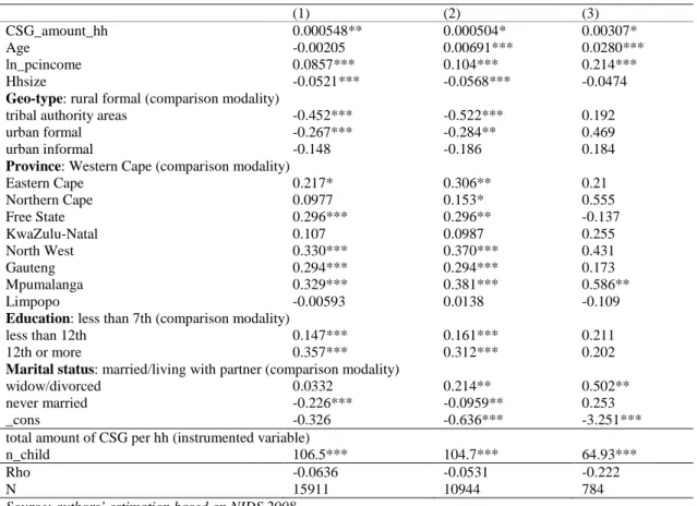
ISCUSSION

Results of the labour force participation model are shown in Table 6. We present three specifications of the model differing only in the sample on which they are run, as described above. The coefficient associated with the total amount received by the household through the CSG is fairly robust across the three specifications. We always find a positive link between the CSG and the probability of participating in the labour force, although, as expected, the coefficient’s value is slightly higher when only people whose youngest children are around the age eligibility threshold are included (model 3). Estimates from specification (1) are finally retained for the simulation analysis.

Table 6: Results of the labour force participation model (1) (2) (3) CSG_amount_hh 0.000548** 0.000504* 0.00307* Age -0.00205 0.00691*** 0.0280*** ln_pcincome 0.0857*** 0.104*** 0.214*** Hhsize -0.0521*** -0.0568*** -0.0474

Geo-type: rural formal (comparison modality)

tribal authority areas -0.452*** -0.522*** 0.192

urban formal -0.267*** -0.284** 0.469

urban informal -0.148 -0.186 0.184

Province: Western Cape (comparison modality)

Eastern Cape 0.217* 0.306** 0.21 Northern Cape 0.0977 0.153* 0.555 Free State 0.296*** 0.296** -0.137 KwaZulu-Natal 0.107 0.0987 0.255 North West 0.330*** 0.370*** 0.431 Gauteng 0.294*** 0.294*** 0.173 Mpumalanga 0.329*** 0.381*** 0.586** Limpopo -0.00593 0.0138 -0.109

Education: less than 7th (comparison modality)

less than 12th 0.147*** 0.161*** 0.211

12th or more 0.357*** 0.312*** 0.202

Marital status: married/living with partner (comparison modality)

widow/divorced 0.0332 0.214** 0.502**

never married -0.226*** -0.0959** 0.253

_cons -0.326 -0.636*** -3.251***

total amount of CSG per hh (instrumented variable)

n_child 106.5*** 104.7*** 64.93***

Rho -0.0636 -0.0531 -0.222

N 15911 10944 784

Source: authors’ estimation based on NIDS 2008

Note: *p<0.10,**p<0.05,***p<0.01; amount of CSG instrumented by n_child (the number of age eligible children); model (1) is estimated on the entire sample of working age people 15-64 (not currently enrolled in school), model (2) on people aged 22-50 (not currently enrolled in school), model (3) on people aged 22-50 (not currently enrolled in school) and living with children aged 12-15 (without younger children)

Table 7 reports the quantity elasticities with respect to own price, expenditure and CSG for each category. They all take the expected sign, revealing an interesting heterogeneity across categories. Fruit and Vegetables, rice, starches and beverages are more responsive to a percent change in their price (more than proportionate reduction), while the own price elasticity for other non-food items is -0.84. Education and other non-food items are found to be superior goods as their demand increase by 1.70 and 1.17% respectively after a percent increase in household expenditure, whereas demand for rice and starches only rise by around 0.60%. Finally, only education and other food categories are found to have a statistically significant CSG elasticity, 1.17 and 1.11 respectively.

Table 7: Quantity elasticities with respect to own price, expenditure and CSG (with t-stat) evaluated at the sample mean

Own Prices Expenditures CSG

Category Elasticity t-stat Elasticity t-stat Elasticity t-stat

Meat -0.95 -21.22 0.78 43.98 0.86 -1.42

Fish -1.11 -1.79 0.73 16.40 0.91 -0.19

Fruit & Vegetables -1.15 -2.06 0.89 38.53 0.96 0.50

Milk -0.96 -1.37 0.98 27.13 0.92 -0.14 Rice -1.20 -3.76 0.58 35.43 0.95 0.45 Starches -1.09 -3.96 0.60 24.84 0.97 0.74 Bread -0.94 -4.43 0.74 29.88 0.84 -1.62 Beverages -1.02 -9.28 0.82 43.51 0.93 -0.09 Education -0.96 -16.07 1.70 34.45 1.17 2.33 Other Food -0.98 -30.35 0.82 38.11 1.11 3.27 Other non-Food -0.84 -2.58 1.17 42.45 0.88 0.79

Source: authors’ estimation based on NIDS 2008

Note: Calculation of elasticities is shown in Appendix 3. Standard errors are calculated with the Delta method. Elasticities values in bold are statistically significant at 5 percent.

Both simulations represent three different shocks that are integrated into the macro model. The shocks only differ by their magnitude between the three simulations. Table 8 summarizes the results of the shocks:

Table 8: Results from the micro model used for the macro model

(Micro) sim1 (Micro) sim2 (Micro) sim3

(Macro) Shock1: change in labour supply (in %, variation)

1.429 1.581 3.342

(Macro) Shock2: change in government transfer received by households (in %, variation) (Macro) Shock3: Change in consumption shares (absolute difference)

Meat -0.00031 -0.00015 -0.00048

Fish 0.00011 0.00005 0.00018

Fruit & Vegetables -0.00007 -0.00004 -0.00012

Milk 0.00002 0.00001 0.00005 Rice -0.00057 -0.00027 -0.00094 Starches -0.00007 -0.00003 -0.00010 Bread -0.00011 -0.00005 -0.00015 Beverages 0.00014 0.00009 0.00031 Education 0.00169 0.00064 0.00234 Other Food 0.00011 0.00009 0.00023 Other non-Food -0.00096 -0.00035 -0.00133

Source: authors’ estimation based on NIDS 2008

As mentioned earlier, there are three shocks that are applied to the CGE model at the same time. Each one of them will have a different impact on the economy. Ceteris paribus, an increase in the labour force would have an impact on unemployment, as it is not feasible for firms to lower wages below the minimum wage. In the same way, an increase of the transfer households receive from government will increase their income and increase government’s deficit11. Finally, the changes in households’ consumption shares will have impacts on final demand.

Volumes of households’ consumption follow the new repartition of the budget shares Table 9. Indeed, education and fish shares are increasing in households’ budget. Ceteris paribus, we expect their volume to increase. On the contrary, meat and rice’s shares are decreasing, so we expect their corresponding demand from households to decrease.

Table 9: Impact on consumption volumes (in%)

sim1 sim2 sim3

Meat -0.91 -0.41 -1.4

Fish 1.09 0.53 1.8

Fruit & Vegetables -0.54 -0.24 -0.83

Milk 0.19 0.13 0.4 Rice -1.57 -0.72 -2.59 Starches -0.65 -0.25 -0.91 Bread -0.34 -0.13 -0.44 Other food 0.28 0.22 0.57 Beverages 0.23 0.17 0.48 Education 4.95 1.93 6.93 Other non-Food -0.04 0.04 0.02

Source: Results from CGE model

11

Indeed, we assume that there is no fiscal policy adjustment to finance the increase of the CSG, and thus this increase, ceteris paribus, will increase government’s deficit

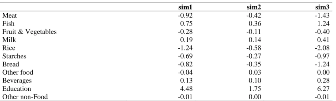
These changes in households’ consumption patterns will have an impact on the production of these sectors. For the alimentary products such as meat and fish commodities, final demand represents between 75 and 95% of the composition of total demand for commodities. Thus, this change in households’ consumption will have a large impact on their production. In contrast, the non-alimentary commodity rely more on intermediate demand from other sectors.

Table 10: Impact on production volumes (in %)

sim1 sim2 sim3

Meat -0.92 -0.42 -1.43

Fish 0.75 0.36 1.24

Fruit & Vegetables -0.28 -0.11 -0.40

Milk 0.19 0.14 0.41 Rice -1.24 -0.58 -2.08 Starches -0.69 -0.27 -0.97 Bread -0.82 -0.35 -1.24 Other food -0.04 0.03 0.00 Beverages 0.13 0.10 0.28 Education 4.48 1.75 6.27 Other non-Food -0.01 0.00 -0.01

Source: Results from the CGE model

As seen in Table 10 production increases, notably in the education sector. The labour intensive educational and diary sectors have to hire more workers for them to increase their production. This can be done in two ways; by hiring workers from other sectors whose production is decreasing or from the increase in the labour supply due to the cash transfer. The overall effect on labour is an increase by 0.04% and 0.05% respectively in the first and second scenarios. In the third scenario, where the two policies are combined, labour increases by 0.08%.

This impact on the labour market, together with the increase in the transfer they receive, results in an increase in households’ income. Since consumption, direct taxes and savings are a proportion of agents' income, they logically increase in all scenarios.

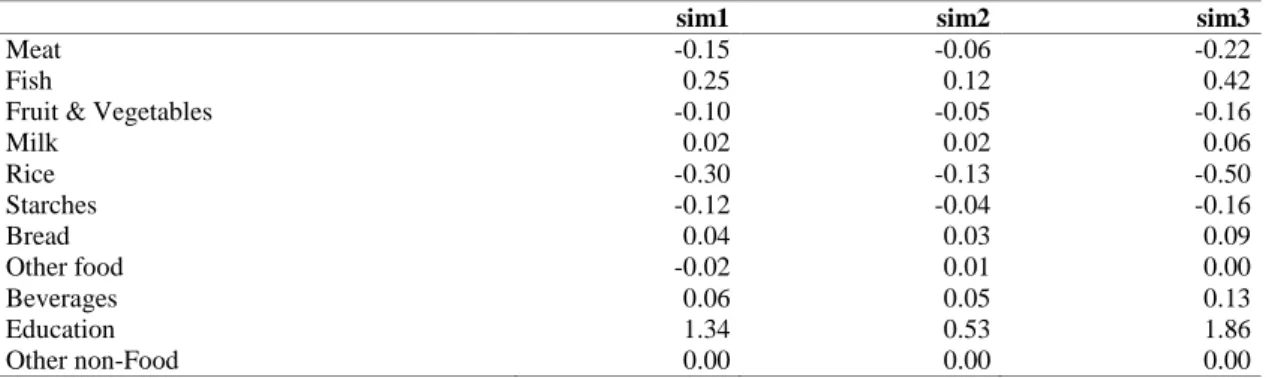
Government’s income increases, due to the increase in direct taxes receipts, as well as on indirect taxes (as consumption increases) and production taxes. However, given the increase in its transfers (i.e. the increase of the CSG), government’s savings are decreasing. This drop has an impact on total investment which decreases. This drop in investment will have an impact on non-alimentary and other food commodities, as they are the only ones which are consumed for investment purposes. The impact on price is hardly perceptible as seen in Table 10. The consumer price index increases very slightly respectively by 0.022%, 0.014%, and 0.03% in the three scenarios.

Table 11: Impact on consumer prices (in %)

sim1 sim2 sim3

Meat -0.15 -0.06 -0.22

Fish 0.25 0.12 0.42

Fruit & Vegetables -0.10 -0.05 -0.16

Milk 0.02 0.02 0.06 Rice -0.30 -0.13 -0.50 Starches -0.12 -0.04 -0.16 Bread 0.04 0.03 0.09 Other food -0.02 0.01 0.00 Beverages 0.06 0.05 0.13 Education 1.34 0.53 1.86 Other non-Food 0.00 0.00 0.00

Source: Results from the CGE model

Before going into the poverty and inequality results, it is noteworthy to discuss briefly the budget cost of the different simulations proposed in this study. Simulation 1 would cost the Government 1.11% of GDP (in 2008 terms), while Simulation 2 and Simulation 3 would cost 1.15% and 1.38% respectively. All the scenarios would call for a significant (probably unrealistic in the case of sim3) effort by the Government in terms of budget increase, as in 2008 the CSG programme cost 0.93% of GDP.

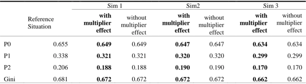
Table 12 to Table 18 report the results for poverty gaps and the inequality Gini index, by different groups. Table 12 and Table 13 show that P0 (Poverty Incidence), P1 (Poverty gap) and P2 (Poverty severity) decrease in comparison with the base year for the whole population and for children respectively. The improvement is particularly strong for poverty severity. As expected from the small changes in the relevant variables discussed above, the multiplier effects on the economy (namely changes in prices, incomes and employment) – other than the direct effect brought by the change in the CSG – have practically no further effects on households’ welfare. This is consistent with the fact that incomes for households living in poverty come primarily from grants and wages. In particular, for households around the poverty line, grants represent around 30% of total incomes while wages account for around 45% (see Figure 1 in Finn, Leibbrandt and Woolard, 2009). In this model, the wage component does not change as the minimum wage binds, and the labour market results are impacted only through unemployment, without significantly affecting the employment rate. The remaining household income share is mostly represented by remittances and rental incomes, which are both unaffected in the short-run of these models. Other incomes and investments only account for a minimal part.

In addition, for the national population, simulations 1 and 2 do not differ substantially, with poverty incidence under sim2 (+ two million beneficiaries) decreasing from 0.532 (base year) to 0.526 (versus 0.528 under sim1 (+20% of CSG value). This is not the case for P1 and P2, for which the two scenarios do not differ in terms of effectiveness of poverty reduction; P1 and P2 go respectively from 0.261 and 0.156 (base year) to 0.250 and 0.145 (under both sim1 and sim2). The Gini index decreases from 0.687 (base year) to 0.682 (under both sim1 and sim2). Interestingly, when we look at results for children only, the effectiveness of sim1 and sim2 in terms of poverty reduction varies according to the poverty measure. Sim2 is found to be more effective in reducing poverty incidence among children as the new 2 million CSG beneficiaries live in households relatively less poor than current beneficiaries, thus being closer to the poverty line. When this group is targeted, a larger reduction in P0 is thus reached, as this measure is sensitive to the density function of the group around the poverty line. Inversely, targeting children already benefiting from the CSG (sim1) allows a greater reduction in poverty depth and poverty severity, as this group – at the base year – is relatively poorer than non-beneficiary children and, thus, further from the poverty line. As well-know, indeed, P1 and, even more, P2 are particularly sensitive to the distributive function of the poor and the poorer tail in particular.