Résolutions coniques des variétés discriminants e applications à la géométrie algébrique complexe et réelle

(1)

HAL Id: tel-00012101

https://tel.archives-ouvertes.fr/tel-00012101

Submitted on 9 Apr 2006

HAL is a multi-disciplinary open access

archive for the deposit and dissemination of

sci-entific research documents, whether they are

pub-lished or not. The documents may come from

teaching and research institutions in France or

abroad, or from public or private research centers.

L’archive ouverte pluridisciplinaire HAL, est

destinée au dépôt et à la diffusion de documents

scientifiques de niveau recherche, publiés ou non,

émanant des établissements d’enseignement et de

recherche français ou étrangers, des laboratoires

publics ou privés.

Résolutions coniques des variétés discriminants e

applications à la géométrie algébrique complexe et réelle

Alexey Gorinov

To cite this version:

Alexey Gorinov. Résolutions coniques des variétés discriminants e applications à la géométrie

al-gébrique complexe et réelle. Mathématiques [math]. Université Paris-Diderot - Paris VII, 2004.

Français. �tel-00012101�

(2)

UNIVERSIT ´

E PARIS 7 - DENIS DIDEROT

UFR de Math´

ematiques

Th`

ese

Pr´esent´ee pour obtenir le diplˆ

ome de

Docteur de l’Universit´

e Paris 7

Spécialité: Mathématiques

Pr´

esent´

ee et soutenue publiquement le vendredi 17 d´

ecembre 2004

par

Alexei Gorinov

R´

esolutions coniques des vari´

et´

es

discriminants et applications `

a la

g´

eom´

etrie alg´

ebrique complexe et r´

eelle

Directeur de th`

ese :

P. Vogel

Rapporteurs :

I. Itenberg

V. Vassiliev

Jury :

V. Kharlamov

S. Orevkov

C. Peters

J. Steenbrink

(3)

(4)

Some conventions and

notation

We shall denote by Πd,n the vector space of complex homogeneous polynomials

of degree d in n + 1 variables, and by Σd,n the subset of Πd,n consisting of

polynomials, whose differential vanishes somewhere in Cn+1_{\ {0}. Set Π} d,n(R)

to be the subset of Πd,n that consists of polynomials with real coefficients.

Unless stated otherwise, we consider only homology and cohomology groups with real coefficients, and the fibers of all local systems are assumed to be real vector spaces of finite dimension.

We shall say that a topological space X is good if the one-point compactifi-cation of X can be provided with the structure of a finite CW -complex. Some statements below that are formulated for good spaces are true in a more general setting, but we shall not need this.

If X is a good topological space, and L is a local system on X, then we shall denote by ¯H_∗(X, L) the Borel-Moore homology groups of X with coefficients in L_{; we set P (X, L) to be the Poincar´e polynomial of X “with coefficients in L”,}

i.e. the polynomialP

iaiti, where ai = dim(Hi(X, L)). In a similar way, we

denote by ¯P (X, L) the polynomialP

iaiti, where ai= dim( ¯Hi(X, L)).

The symbol “⊂” denotes an inclusion; a strict inclusion is denoted by “(”. As usual, if X is a topological space, and A ⊂ X, we denote by ¯A the closure of A in X.

If f : X → Y is a continuous map of topological spaces, and A and B are sheaves on X and Y respectively, then we denote by f∗(A), respectively, by

f−1_{(B) the direct image of A, respectively the inverse image of B, under f .}

The symbol “#” denotes the cardinality of a finite set.

The symbol “\” denotes the difference of two sets and never the left quotient; we write X/G for the quotient of a manifold X by an action of a group G, regardless whether the action is right or left.

The symmetric group on k elements is denoted by Sk everywhere except the

appendix, where it is denoted by Sk, and Sk means something else.

We systematically use the “topological” notation instead of the “algebraic” one, e.g., we write CPn _{and Z}

2, and not Pn(C) and Z/2Z etc.

“Random” symbols like X, A, x, a, f etc. may have different meanings in dif-ferent chapters (and sometimes even within the same chapter); we hope however that this never leads to a confusion.

(7)

Acknoledgements

First of all, I must thank V. A. Vassiliev who introduced me into the study of discriminant complements. Most of the thesis is based on his ideas, and without his encouragement and support this thesis would not have been written.

I am very much indebted to my advisor at Paris 7, Pierre Vogel, for various support and so many useful conversations, which contributed greatly to my topological education.

I would like to thank E. G. Sklyarenko, my first advisor many years ago back in Moscow.

I wish to thank the anonymous referee who read the paper [6] and made many valuable remarks.

Many thanks go to Andrei Inshakov and Alexei Oblomkov from whom I learnt most of algebraic geometry I know, and to Yann Sepulcre for a crash course in dualising sheaves.

I wish to thank J. Steenbrink for interest in my work and many useful dis-cussions. I am grateful to V. I. Arnold, I. V. Itenberg, V. M. Kharlamov and C. Peters for useful conversations, and for giving me a chance to speak at their seminars, and to A. Goncharov, E. Looijenga and O. Ya. Viro for useful corre-spondence.

Neither the last, not the least, I wish to thank Sergei Shadchin, Alexandre Engoulatov and other people who supported me in this way or another during hard times in my life.

I am grateful to my father who did for me what I had to do myself, but couldn’t, and to my mother for everything.

(8)

Chapter 1

Introduction

Considérons la situation suivante : soit V un espace affine dont les éléments paramétrisent des fonctions définies sur une certaine variété. Souvent ces fonc-tions se partagent en génériques et singulières (la définition de ce que l’on appelle “singulier” varie selon le cas). Le sous-espace (topologique) Σ de V constitué des fonctions singulières est appelé un discriminant (généralisé).

Beaucoup d’espaces topologiques “célèbres” sont des complémentaires de discriminants (ou sont homotopiquement équivalents à des complémentaires de discriminants). On peut mentionner comme exemples les groupes de Lie classiques matriciels, les espaces de nœuds, les espaces d’applications lisses sans singularités compliquées, les espaces classifiants des groupes de tresses, les complémentaires d’arrangements de sous-espaces affines de dimensions quel-conques, les espaces d’applications lisses entre des sphères, etc. Les questions concernant la géométrie et la topologie des complémentaires de discriminants se posent donc dans des situations très diverses.

Une stratégie générale pour calculer la cohomologie du complémentaire d’un discriminant a été introduite par V. A. Vassiliev il y a plus de 15 ans. Cette stratégie s’est avérée très efficace ; en plus de donner beaucoup de nouveaux résultats (comme les invariants de Vassiliev des nœuds), elle fournit une expli-cation unifiée pour certains faits qui n’ont pas de liens apparents (comme la formule de Goresky-MacPherson qui calcule la cohomologie d’un arrangement de k-plans, la suite spectrale d’Adams pour la cohomologie des espaces de lacets, le théorème de Snaith sur le scindage de la cohomologie des groupes de Lie, etc.). Expliquons brièvement comment cette stratégie marche dans le cas élémen-taire suivant : soit V l’espace des polynômes xd_{+ a}

d−1xd−1+ · · · + a0, o`u d est

un entier fixé supérieur ou égal à 2, et les ai sont des réels. Notons Σ le

sous-ensemble de V formé des polynômes ayant une racine multiple. Par la dualité d’Alexander, le calcul des groupes do cohomologie H∗_{(V \ Σ) est ramené au}

calcul des groupes d’homologie de Borel-Moore de Σ. La question qui se pose alors est le calcul de ces groupes d’homologie. Il existe une r´esolution lisse ´evidente Σ′ _{de Σ : on pose}

Σ′= {(f, x)|f ∈ Σ, x ∈ R, f (x) = f′(x) = 0}.

Malheureusement, la projection Σ′ _{→ Σ n’induit presque jamais un}

iso-morphisme au niveau de l’homologie de Borel-Moore, puisque, par exemple, si d > 3, il existe des polynˆomes ayant deux racines doubles, et on les compte

(9)

4 CHAPTER 1. INTRODUCTION alors deux fois en haut. Peu importe, se dit-on, et pour tout f ayant plus d’une racine multiple, et pour tous x1 6= x2 deux racines multiples de f , on recolle

formellement un segment reliant (f, x1) et (f, x2). L’espace Σ′′ obtenu ainsi

se projette lui aussi sur Σ, mais cette fois-ci ce sont les polynômes ayant au moins 3 racines multiples distinctes qui posent problème : si, par exemple, un polynôme a exactement trois racines multiples distinctes, sa préimage est un cer-cle (topologique). Pour tout f ayant au moins trois racines multiples distinctes, et tous x1, x2, x3 racines multiples distinctes de f , on recolle donc comme tout

`

a l’heure un 2-simplexe dont les sommets sont (f, x1), (f, x2), (f, x3). On

repro-duit cette procédure si nécessaire avec des simplexes de dimension supérieure à 2 jusqu’à ce que tous les générateurs indésirables de l’homologie en haut soient tués.

L’espace σ obtenu ainsi est appelé la résolution simpliciale de Σ. L’intérêt d’utiliser σ plutôt que Σ provient du fait que σ admet une filtration naturelle que l’on a en fait construite au cours de la bataille avec les générateurs d’homologie redondants :

∅⊂ Σ′⊂ Σ′′⊂ · · · ⊂ σ.

La différence de deux termes consecutifs dans cette filtration est un fibré vec-toriel au-dessus de l’espace des configurations non ordonnées de k points de R. Cela permet d’écrire immédiatement le terme E1 _{de la suite spectrale}

corre-spondant à cette filtration. Cette suite spectrale dégénère au premier terme et donne les groupes d’homologie de Borel-Moore de Σ.

Une source naturelle d’exemples de complémentaires de discriminants est fournie par la géométrie algébrique où les espaces d’hypersurfaces projectives lisses sont des objets d’étude classiques. Les espaces de modules de courbes de petit genre se décomposent canoniquement en morceaux dont chacun est le quo-tient du complémentaire d’un discriminant par l’action d’un groupe algébrique. Dans l’article [14], V. A. Vassiliev a expliqué comment sa stratégie s’applique au cas des hypersurfaces projectives lisses.

La majeure partie de la thèse est consacrée à une généralisation de cette

méthode. En gros, nous présentons une méthode inspirée de [14] (plus

précisément, des calculs faits dans [14]) qui nous permet dans certains cas d’aller un peu plus loin, par exemple, en augmentant le degré ou la dimension de l’espace ambiant, ou le genre etc. On présente également quelques applications. La liste des applications que l’on présente n’est pas exhaustive1 _{; elle ne}

con-tient pas non plus tous les cas intéressants (l’application la plus intéressante de la méthode présentée ici est probablement le calcul du polynôme de Poincaré de M₄_{par O. Tommasi dans [13]; l’auteur a fait le même calcul indépendamment,} mais plus tard). Ces applications sont données dans le seul but de montrer les problèmes que l’on peut résoudre en utilisant notre méthode.

Par ailleurs, il faut remarquer que cette méthode n’a donné (au moins pour l’instant) aucun résultat sur la cohomologie des espaces d’hypersurfaces de degré

1_{Par exemple, l’auteur a r´}_{ecemment calcul´}_{e les polynˆ}_{omes de Poincar´}_{e des quotients des}

espaces des quartiques nodales et GIT-stables par l’action ´evidente du groupe P GL3(C). Les

r´eponses sont respectivement 1+t2_+t4_+t6_{et 1+t}2_+2t4_+2t6_+t7_+t8_{; malheureusement, ces}

calculs ont été terminés trop tard pour être inclus dans la thèse. Le premier de ces résultats permet de montrer que le polynôme de Poincaré de l’espace ¯M3des courbes

Deligne-Mumford-stables de genre 3 est ´egal `a 1+3t2_+7t4_+10t6_+7t8_+3t10_+t12_{. Ce r´}_{esultat n’est pas nouveau}

(cf. [4, page 19] ; je remercie J. Steenbrink et O. Tommasi pour cette référence), mais notre démonstration est indépendante. Le seul fait non trivial que l’on utilise est H5

( ¯M3) = 0, ce

(10)

5 quelconque, ou des espaces de modules de courbes de genre quelconque; elle ne donne pas non plus beaucoup d’information sur les groupes fondamentaux des complémentaires de discriminants (puisque notre premier pas consistera à rem-placer le calcul des groupes de cohomologie du complémentaire à un discriminant par le calcul des groupes d’homologie de Borel-Moore du discriminant même).

La thèse est organisée de la manière suivante : dans le chapitre 3 on rap-pelle la construction de V. A. Vassiliev [14], on explique quel est l’intérêt de la généraliser, et on présente notre construction. Dans le chapitre 4 on donne quelques résultats homologiques dont on aura besoin dans la suite. Les chapitres suivants sont consacrés aux applications: dans le chapitre 5 on considère le cas des quintiques de CP2 _{(le discriminant est une hypersurface irréductible), dans}

le chapitre 6 on calcule les nombres de Betti de l’espace des cubiques lisses qui intersectent transversalement une conique lisse fixée (le discriminant est réductible, mais la méthode marche aussi bien), dans le chapitre 7 on considère l’espace des cubiques lisses réelles (cet espace peut sûrement être consideré en utilisant une technique plus standard, toutefois on présente nos calculs comme un exemple test dans le cas réel).

Certains résultats de la thèse ont été annoncés dans [5]; un texte contenant la construction de la résolution conique et l’une des applications mentionnées dessus (le cas des quintiques projectives planes) a été accepté [6].

La thèse contient un appendice reproduisant l’article [7]. On y démontre le théorème suivant : supposons que le cercle est muni d’un atlas où toutes les fonctions de changement de cartes sont des homographies ; alors ce cercle borde une surface orientable munie d’un atlas où toutes les fonctions de changement de cartes sont des homographies (à coefficients complexes cette fois-ci) compatibles dans le sens évident avec les applications de changement de cartes sur le bord. On y établit également une classification correcte des cercles projectifs (il s’avère que la classification trouvée il y a longtemps par N. Kuiper est incomplète).

(11)

Chapter 2

Introduction

Consider the following situation: suppose we are given an affine space V , whose elements parametrise functions defined on some manifold. Usually, these func-tions can be divided into generic and singular (the definition of “singular” varies from case to case). The subspace Σ of V that consists of the singular functions is called a (generalised) discrimimant.

Many “famous” topological spaces (such as classical matrix Lie groups, spaces of knots, spaces of smooth maps between spheres, classifying spaces of braid groups, complements of arrangements of planes of different dimensions, spaces of smooth maps without complicated singularities, just to mention a few examples) are discriminant complements (or are homotopy equivalent to discriminant complements), so questions concerning geometry and topology of discriminant complements arise in many different situations.

A general strategy of calculating cohomology groups of discriminant com-plements was introduced by V. A. Vassiliev over 15 years ago. This strategy turned out to be very effective; apart from giving many new results (such as Vassiliev knot invariants), it also provides a unified explanation for some seem-ingly unrelated facts (such as Goresky-MacPherson formula for the cohomology of the complement of a plane arrangement, Adams spectral sequence for the cohomology of loop spaces, the Snaith splitting theorem for the cohomology of classical Lie groups and some others).

Let us briefly explain how this strategy works in the following elementary example: let V be the space of polynomials of the form xd_{+ a}

d−1xd−1+ · · ·+ a0,

where d is some fixed integer > 1 , and the ai’s are real numbers; set Σ to be

the subset of V that consists of the polynomials with multiple roots. Via the Alexander duality we can replace the calculation of the groups H∗_{(V \ Σ) by}

the calculation of the Borel-Moore homology groups of Σ. But how can that be done? There is an obvious smooth resolution Σ′ _{of Σ: we set}

Σ′= {(f, x)|f ∈ Σ, x ∈ R, f (x) = f′(x) = 0}.

Unfortunately, the projection Σ′_{→ Σ almost never induces an isomorphism}

of the Borel-Moore homology groups, since, e.g., if d > 3, there are polynomials that have two multiple roots, and they are counted twice upstairs. “Never mind” – we say, and formally glue the segment that joins (f, x1) and (f, x2)

for any f that has more than one multiple root, and any two multiple roots x16= x2 of f . The resulting space Σ′′ also projects onto Σ, but this time it is

(12)

7 the polynomials with ≥ 3 distinct multiple roots that cause troubles: e.g., the preimage of a polynomial that has exactly three multiple roots is (topologically) a circle. So we proceed as above and glue in the triangle spanned by the points (f, x1), (f, x2), (f, x3) for any f that has three or more multiple roots, and any

(unordered) triple x1, x2, x3 of distinct multiple roots of f , and so on until all

unwished homology generators upstairs are killed.

The resulting space σ is called the simplicial resolution of Σ. The point of us-ing σ rather than Σ consists in the fact that σ admits a natural filtration, which we have already constructed while fighting the redundant homology classes:

∅⊂ Σ′_{⊂ Σ}′′_{⊂ · · · ⊂ σ.}

The difference of any two consecutive terms of this filtration is a vector bundle over the space of unordered k-ples of points in R, which enables us immediately

to write down the term E1 _{of the spectral sequence that corresponds to the}

filtration. This spectral sequence degenerates at the first term, and gives us immediately the Borel-Moore homology groups of Σ.

A natural source of examples of discriminant complements is provided by algebraic geometry, where spaces of smooth projective hypersurfaces are classi-cal objects of study. Moduli spaces of curves of small genus can be canoniclassi-cally decomposed into several pieces, so that each piece is the quotient of a discrimi-nant complement by the action of some algebraic group. In the article [14] V. A. Vassiliev explained how to apply his strategy to the case of smooth projective hypersurfaces.

The main part of the thesis is devoted to a generalisation of that method. Roughly speaking, we present a method inspired by [14] (more precisely, by the calculations performed in [14]), which enables one in some cases to go one step further, i.e., to increase by one the degree or the dimension of the ambient space or the genus etc. We also present some applications. The list of applications is not exhaustive1 _{nor does it contain r all interesting cases (the most interesting}

application so far of the method presented here is probably the calculation of

the Poincar´e polynomial of M4 performed by O. Tommasi in [13]; the author

has done the same calculation independently but later). The only point in presenting these applications is to show what problems can be handled using our method.

It should be noted by the way that (at least at present) this method does not give any results about the cohomology of spaces of hypersurfaces of arbitrary degree, or moduli spaces of curves of arbitrary genus; nor does it give much information on the fundamental groups of discriminant complements (since our first step will as above consist in replacing the calculation of the cohomology groups of a discriminant complement by the calculation of the Borel-Moore homology groups of the discriminant itself).

1_{For instance, the author has recently calculated the Poincar´}_{e polynomials of the quotients}

of the spaces of nodal and GIT-stable plane quartics by the obvious action of the group P GL3(C). The answers are respectively 1 + t2+ t4+ t6 and 1 + t2+ 2t4+ 2t6+ t7+ t8;

unfortunately these calculations were completed too late to be included in the thesis. The first one of these results enables one to show that the Poincar´e polynomial of the space ¯M3of

Deligne-Mumford-stable genus 3 curves is 1 + 3t2_{+ 7t}4_{+ 10t}6_{+ 7t}8_{+ 3t}10_{+ t}12_{. This result is}

not new (see [4, page 19]; I am grateful to J. Steenbrink and O. Tommasi for this reference), but our proof is independent. The only nontrivial fact we use is H5

( ¯M3) = 0, as shown by E.

(13)

8 CHAPTER 2. INTRODUCTION The thesis is organised as follows: in chapter 3 we recall V. A. Vassiliev’s construction from [14], give some argument why it should be generalised and then present our construction. In chapter 4 we give some homological results that we shall need in the sequel. The remaining chapters are devoted to ap-plications: in chapter 5 we consider the case of smooth quintics in CP2 _(the

discriminant is an irreducible hypersurface), in chapter 6 we calculate the Betti numbers of the space of smooth plane cubics that intersect transversally a fixed smooth conic (the discriminant is reducible, but the method works just as well), in chapter 7 we consider the space of smooth real plane cubics (this space can surely be considered using some more standard technique, but we present our calculations as a test example in the real case).

Some of the results of the thesis were announced in [5]; a text containing the construction of the conical resolution and the first of the above-mentioned applications (the spase of smooth plane projective quintics) has been accepted [6].

The thesis contains an appendix, which reproduces the article [7]. Roughly speaking, we prove the following theorem: suppose the circle is equipped with an atlas, where all transition maps are fractional linear; then this circle bounds an orientable surface with an atlas where all transition maps are also fractional linear (only this time with complex coefficients) and are compatible in the ob-viuous way with the transition maps on the boundary. We also show that the classification of projective circles given long ago by N. Kuiper is not quite correct and give a correct one.

(14)

Chapter 3

The method of conical

resolutions

3.1 Why generalise?

In this chapter we describe a general method of computing (at least additively) the cohomology groups of spaces like Πd,n\Σd,n. Our method is a generalisation

of the one given in [14]. Everyone who proposes to generalise something has to face the question that is the title of this section. In order to answer this question, let us recall briefly V. A. Vassiliev’s construction from [14, Section 2].

Suppose that we are interested in calculating the cohomology groups of Πd,n\

Σd,n. The first remark is the following: via the Alexander duality we have

Hi(Πd,n\ Σd,n) ∼= ¯H2D−i−1(Σd,n),

where D = dimC(Πd,n). This reduction was first used by V. I. Arnold in [2]. The

variety Σd,n is usually very singular, and there seems to be no immediate way

to compute its Borel-Moore homology groups. In order to do this, we construct a space ˜σd,n called the conical resolution of Σd,n. We shall see that, on the one

hand, there is a natural proper map π : ˜σd,n→ Σd,n such that the preimage of

any point of Σd,n is a cone (hence the term “conical”), and on the other hand,

˜

σd,n admits a very nice filtration, which enables one to calculate the groups

¯

H_∗(˜σd,n) for some values of d and n. The space ˜σd,n is constructed as follows.

For any K ⊂ CPn _{denote by L(K) the vector subspace of Π}

d,n

consist-ing of all polynomials that have sconsist-ingular points everywhere in K (and maybe elsewhere). For any i = 1, . . . , D denote by Gi(Πd,n) the Grassmann manifold

whose points are complex subspaces of Πd,nof codimension i. Denote by Ωi the

subspace of Πd,n consisting of all vector subspaces that have the form L(K),

where K is the set of singular points of some polynomial from Σd,n.

A simplex of the join

G1(Πd,n) ∗ G2(Πd,n) ∗ · · · GD(Πd,n)

is called coherent, if its vertices form a flag. The main vertex of a coherent simplex △ is the vertex corresponding to the smallest subspace among the sub-spaces that correspond to the vertices of △. The union of all coherent simplices

(15)

10 CHAPTER 3. THE METHOD OF CONICAL RESOLUTIONS with vertices in ¯Ωi is denoted by ˜Λd,n (here ¯Ωi stands for the closure of Ωi in

Gi(Πd,n)). For any L ∈ ¯Ωidenote by ˜Λd,n(L) the union of all coherent simplices

whose main vertex is L. Every space ˜Λd,n(L) is a cone with vertex L; denote

the base of this cone by ∂ ˜Λ(L).

Set ˜σd,n to be the subspace of Σd,n× ˜Λd,nthat consists of all couples (f, x)

such that f ∈ L and x ∈ ˜Λd,n(L), where L ∈ ¯Ωi for some i = 1, . . . , D. Set

˜

Φi to be the union of all coherent simplices whose main vertices belong to

S

j≤iGj(Πd,n), and set

Fi = {(f, x) ∈ ˜σd,n|x ∈ ˜Φi}.

We have the filtrations

∅⊂ ˜Φ1⊂ · · · ˜ΦD= ˜Λd,n (3.1)

and

∅⊂ F1⊂ · · · FD= Σd,n. (3.2)

Theorem 3.1 1. The obvious projection π : ˜σd,n → Σd,n is a proper map

and induces an isomorphism of Borel-Moore homology groups.

2. The space Fi\ Fi−1 is a (D − i)-dimensional complex vector bundle over

˜

Φi\ ˜Φi−1.

So via the Thom isomorphism the task of writing down the term E1 _{of the}

spectral sequence corresponding to the above filtration on ˜σd,n is reduced to

calculating the Borel-Moore homology groups of the spaces ˜Φi\ ˜Φi−1. There

exists for any i = 1, . . . , D the obvious map ˜Φi\ ˜Φi−1 → ¯Ωi such that for any

L ∈ ¯Ωi the preimage of L is the open cone ˜Λd,n(L) \ ∂ ˜Λd,n(L). Usually one has

to stratify ¯Ωi so that the above map becomes the projection of a locally trivial

bundle over each stratum.

It turns out that for any L ∈ ¯Ωi\ Ωi the space ∂ ˜Λd,n(L) is contractible, and

for L ∈ Ωi we have

¯

H_∗(˜Λd,n(L) \ ∂ ˜Λd,n(L)) ∼= ¯H∗(Λd,n(L) \ ∂Λd,n(L)),

where Λ(L) and ∂Λ(L) are obtained by taking the union of all coherent simplices (respectively from ˜Λ(L) and ∂ ˜Λ(L)), all of whose vertices belong to Ωj, j ≤ i.

So, in order to write down the term E1_{of the spectral sequence corresponding}

to (3.2), we have to know the Borel-Moore homology groups of certain fibre bundles over certain subvarieties of the Ωi’s.

However, sometimes the fibres or the bases of these bundles turn out to be quite complicated. Consider, e.g., the case of Π5,2. We have then D = 21. The

space Ω20 is stratified as follows: Ω20= Ω120⊔ Ω220⊔ Ω320Ω420, where Ω120, . . . , Ω420

correspond respectively to the following singular curves: five lines in general position, three lines and a smooth conic in general position, two smooth conics and a line in general position, and two lines and an irreducible singular cubic in general position (in the last case “in general position” means that the cubic intersects each line at three distinct points, none of which is the intersection point of the lines).

Let us describe the space ∂Λ5,2(L) for L ∈ Ω120. The vector space L is

(16)

3.2. THE CONSTRUCTION OF THE CONICAL RESOLUTION 11 position; denote by K the set of ten intersection points of those lines. Denote by △ the 9-dimensional simplex, whose vertices formally correspond to the elements of K. Define a mapping ∂Λ5,2(L) → △ as follows: take every L(K′), K′ ⊂ K

to the barycentre of the face of △ spanned by the elements of K′_{, and extend}

linearly to all coherent simplices ⊂ ∂Λ5,2(L). This mapping is a homeomorphism

on its image.

It can be proven using lemma 5.1 below that minimal vector spaces that contain L and have the form L(K), where K is the singular locus of some quintic, are

1. L(four points on l + three points in general position outside l), and 2. L(three points on l1\ l2plus three points on l2\ l1plus l1∩ l2),

where l, l1, l2 are lines, l1 6= l2. One can show that the image of the above

mapping can be contracted onto the union U of the images of Λ5,2(L′), where

L′ _{is of the first type. U is the union of all 6-faces of △ that are opposite to the}

2-faces spanned by triples of points on a line.

There exists a natural action of the symmetric group S5on H∗(U ), and most

irreducible representations of S5 occur in the corresponding decomposition of

H∗(U ). Hence, in order to find the contribution of Ω120, it is necessary to

calcu-late the Borel-Moore homology of Ω1

20 with coeficients in many local systems.

The same holds for the spaces Ω2

20 etc.; calculating the contribution in these

cases appears to be an even more difficult task, since the conditions that define these spaces are nonlinear.

Luckily, there is a way to overcome some of these difficulties. Below we present another version of the conical resolution. The main difference can be informally summarised as follows: we define coherent simplices using inclusions between singular loci themselves, rather then between the corresponding vector spaces. This gives us more flexibility in comparison with the above method, but forces us to introduce lots of “fake” singular loci, which we count once with a plus, and once with a minus.

3.2 The construction of the conical resolution

Let V be a vector space of k-valued functions on a manifold M and Σ ⊂ V is a closed subspace formed by the functions that are singular in some sence. (The space Σ is often called a discriminant; in all examples that we shall consider

Σ will be an algebraic variety.) Suppose that D = dimkV < ∞. We want

to calculate the Borel-Moore homology of Σ. In order to do this, we preceed as above, i.e., we construct a resolution σ and a proper map π : σ → Σ such that the preimage of every point is contractible. We are going to describe a construction of σ via configuration spaces.

Remark. The method described below can be extended with obvious mod-ifications to the case when V is an affine space. We assume V to be a vector space, since, on the one hand, the vector case is somewhat simpler, and on the other hand it is sufficient for all applications that we have in mind.

Suppose that with every function f ∈ Σ a compact nonempty subset Kf

of some compact CW -complex M is associated. For instance, if M = Cn+1_\

(17)

12 CHAPTER 3. THE METHOD OF CONICAL RESOLUTIONS the image of the set of singular points of f under the natural map M → CPn. We suppose that the following conditions are satisfied:

• If f, g ∈ Σ, and Kf∩ Kg6= ∅, then f + g ∈ Σ and Kf∩ Kg⊂ Kf +g,

• If f ∈ Σ, then for any λ 6= 0 we have Kλf = Kf,

• The zero function 0 ∈ Σ, and K0= M .

• For any K ⊂ M set L(K) ⊂ V to be the subset consisting of all f such that

K ⊂ Kf. The previous three conditions imply that L(K) is a k-vector

space. We suppose that there exists a positive integer d such that for any x ∈ M one can find a neighbourhood U ∋ x in M and continuous functions l1, . . . , ld from U to the Grassmannian GD−1(V ) of (D − 1)-dimensional

k-vector subspaces of V such that we have L({x′}) = d \ i=1 li(x′) for any x′_{∈ U .}

Remark. One may ask a natural question: if we are dealing with functions on some manifold M, why should we introduce some additional space M? The problem is that for our construction it will be convenient to associate with a singular function a compact subset of a compact CW -complex. In the case when the manifold M itself is compact, we can assume, of course, that M = M, and Kf is the singular locus of f (the definition of the singular locus depends on the

particular example we are considering).

By a configuration in a compact CW -complex M we shall mean a compact

nonempty subset of M. Denote by 2M _{the space of all configurations in M.}

Suppose that ρ is the metric on M. We introduce the Hausdorff metric on 2M

by the usual rule: ˜

ρ(K, L) = maxx∈Kρ(x, L) + maxx∈Lρ(x, K).

The resulting topology on 2M _{does not depend on the choice of the particular}

metric that induces the topology on M.

It is easy to check that if M is compact, then the space 2M_{equipped with}

the metric ˜ρ is also compact.

Notation. We denote by B(M, k) the subspace of 2M _{that consists of all}

configurations that contain exactly k elements.

Note that we have B(M, k) =S

j≤kB(M, j).

Proposition 3.1 Let (Kj) be a Cauchy sequence in 2M, and let K be the set

consisting of the limits of all sequences (aj) such that aj ∈ Kj for every j. Then

K is nonempty and compact, and limj→∞ρ(K˜ j, K) = 0.

♦

Proposition 3.2 Let (Ki), (Li) be two sequences in 2M. Suppose that there

exist limi→∞Ki, limi→∞Li, and denote these limits by K and L respectively.

(18)

3.2. THE CONSTRUCTION OF THE CONICAL RESOLUTION 13 ♦

Suppose that X1, . . . , XN is a finite collection of subspaces of 2Msatisfying

the following conditions:

1. For every f ∈ Σ the set Kf belongs to some Xi.

2. Suppose that K ∈ Xi, L ∈ Xj, K ( L. Then i < j.

3. Recall that L(K) is the space of all functions f such that K ⊂ Kf. Let us

fix i; we assume that dimkL(K) is the same for all configurations K ∈ Xi.

(We denote this dimension by di.)

4. Xi∩ Xj= ∅ if i 6= j.

5. For any i the space ¯Xi\ Xi is included inSj<iXj.

6. For every i we denote by Ti the subspace of M × 2M consisting of pairs

(x, K) such that K ∈ Xi and x ∈ K. We assume that Ti is the total

space of a locally trivial bundle over Xi (the projection pri : Ti → Xi is

obvious). This bundle will be called the tautological bundle1 _{over X} i.

7. Note that any local trivialisation of Ti has the following form:

(x, K′) 7→ (t(x, K′), K′).

Here x is a point in some K ∈ Xi, K′ belongs to some neighbourhood

U ∋ K in Xi, and t : K × U → M is a continuous map such that if we

fix K′ _{∈ U , then we obtain a homeomorphism t}_K_′ _{: K → K}′_{. We require}

that for every K ∈ Xi there exist a neighbourhood U ∋ K and a local

trivialisation of Ti over U such that every map tK′ : K → K′ establishes

a bijective correspondence between the subsets of K and K′ _{that belong}

toS

j≤iXj.

Under these assumptions we are going to construct a resolution σ of Σ and a filtration on it such that the i-th term of the filtration is the total space of a fibre bundle over Xi.

Note that due to condition 3 for any i = 1 . . . , N there exists an natural map K 7→ L(K) from Xi to the Grassmann manifold Gdi(V ), which is continuous

due to the last condition from the list on page 12.

Remark. The rather strange-looking condition 7 follows immediately from condition 6 in the following situation: suppose Xi consists of finite

configura-tions, and for all K, L, such that K ∈ Xi, L ⊂ K there is an index j < i such

that L ∈ Xj. In this case any trivialisation of Ti fits.

Let us now recall the notion of the k-th self-join of a topological space. This notion was introduced by V.A. Vassiliev in [14] and will come out very useful on several occasions in the sequel.

Definition. Let X be a topological space that can be embedded into a finite dimensional Euclidean space, and let k be a positive integer. We shall say that a proper embedding ı : X → RΩ_{, Ω < ∞, is k-generic, if the intersection of any}

1

For instance, if M = CPn

and Xi consists of projective subspaces of M of the same

dimension, then this is just the projectivisation of the usual tautological bundle over the corresponding subvariety of some Grassmann manifold of Cn+1_.

(19)

14 CHAPTER 3. THE METHOD OF CONICAL RESOLUTIONS two (k − 1)-simplices with vertices on ı(X) is their common face (in particular, the intersection is empty, if the sets of the vertices are disjoint). We set the k-th self-join X∗k _{of X to be the union of all (k − 1)-simplices with vertices on the}

image ı(X) of any k-generic embedding ı. For good spaces this definition does not depend on the choice of ı.

Consider the space Y =SN

i=1X¯i=

SN

i=1Xi. Denote by X the N -th self-join

Y∗N _{of Y Note that the spaces Y, Y}∗N _{are compact. Call a simplex △ ⊂ X}

coherent if the configurations corresponding to its vertices form an ascending sequence. Note that then its vertices belong to different Xi (condition 2). Let

△ be a coherent simplex. Among the vertices of △ there is a vertex such that the corresponding configuration contains the configurations that correspond to all other vertices of △. Such vertex will be called the main vertex of △. Denote by Λ the union of all coherent simplices. For any K ∈ Xi denote by Λ(K) the

union of all coherent simplices, whose main vertices coincide with K. Note that the space Λ(K) is contractible.

Denote by Φi the unionS_j≤iS_K∈X_jΛ(K). There is a filtration on Λ: ∅ ⊂

Φ1⊂ · · · ⊂ ΦN = Λ.

For any simplex △ ⊂ X denote by△ its interior, i.e. the union of its points◦ that do not belong to the faces of lower dimension. Note that for every x ∈ X there exists a unique simplex △ such that x ∈△.◦

Proposition 3.3 Let (xi) be a sequence in X such that limi→∞xi= x. Suppose

xi ∈ △i, x ∈ ◦

△, where △i are coherent simplices, and suppose K is a vertex

of △. Then there exists a sequence (Ki) such that Ki is a vertex of △i and

limi→∞Ki= K.

♦

Proposition 3.4 All spaces Λ, Λ(K), Φi are compact.

Proof. This follows immediately from propositions 3.3 and 3.2. ♦

For any K ∈ Xi denote by ∂Λ(K) the union SκΛ(κ) over all maximal

subconfigurations κ ∈ ∪j<iXj, κ ( K. The space Λ(K) is the union of all

segments that join points of ∂Λ(K) with K, and hence it is homeomorphic to the cone over ∂Λ(K).

Define the conical resolution σ as the subspace of Σ × Λ consisting of pairs (f, x) such that f ∈ Σ, x ∈ Λ(Kf).

Proposition 3.5 The space σ is closed in Σ × Λ.

Proof. Let (fi, xi) be a sequence such that all fi∈ Σ, every xi ∈ Λ(Kfi), and

we have limi→∞fi = f ∈ Σ, limi→∞xi= x ∈ Λ. Let us prove that x ∈ Λ(Kf).

Let △ be the coherent simplex such that x ∈△. Due to proposition 3.3, there◦ exists a sequence (Ki) such that all Ki ∈ Y and Ki ⊂ Kfi. Take an element

a ∈ K. By proposition 3.1, there exists a sequence (ai) of elements of M such

that lim_i→∞ai = a. For any i, we have Fi ∈ L(Ki) ⊂ L({ai}). Due to the

last condition from the list on page 12, f ∈ L({a}). So, for any a ∈ K we have a ∈ Kf, which means that K ⊂ Kf. The proposition is proven.♦

There exist obvious projections π : σ → Σ and p : σ → Λ. We introduce a filtration on σ putting Fi = p−1(Φi). The map π is proper; indeed, by

(20)

3.2. THE CONSTRUCTION OF THE CONICAL RESOLUTION 15 proposition 3.5, the preimage of each compact set C ⊂ Σ is a closed subspace of C × Λ, which is compact.

Theorem 3.2 Suppose X1, . . . , XN are subspaces of 2Mthat satisfy Conditions

1–7 of page 13. Then

1. π induces an isomorphism of Borel-Moore homology groups of the spaces σ and Σ.

2. Every space Fi\ Fi−1 is a k-vector bundle over Φi\ Φi−1 of dimension di.

3. The space Φi\Φi−1is a fibre bundle over Xi, the fibre being homeomorphic

to Λ(K) \ ∂Λ(K).

Proof. The first assertion of the theorem follows from the fact that π is proper and π−1_{(f ) = Λ(K}_f_{), the latter space being contractible. To prove the}

second assertion, let us study the preimage of a point x ∈ Φi\ Φi−1 under the

map p : Fi\ Fi−1→ Φi\ Φi−1. We claim that p−1(x) = L(K) for some K ∈ Xi.

Recall that each point x ∈ Φi\ Φi−1belongs to the interior of some coherent

simplex △, whose main vertex lies in Xi. Denote this vertex by K and denote

the map Φi\ Φi−1 ∋ x 7→ K ∈ Xi by fi.

Now suppose f ∈ L(K), or, which is the same, Kf ⊃ K. This implies

Λ(K) ⊂ Λ(Kf). So we have x ∈ Λ(K) ⊂ Λ(Kf) and (f, x) ∈ σ, p(f, x) = x,

hence f ∈ p−1_(x).

Suppose now that f ∈ p−1_{(x). We have (f, x) ∈ σ, hence x ∈ Λ(K}_f_{). This}

means that x belongs to some coherent simplex △′_{, whose main vertex is K} f.

But x belongs to the interior of △, hence △ is a face of △′ _{and K is a vertex of}

△′_{. But K}

f is the main vertex of △′, hence K ⊂ Kf and f ∈ L(K).

So, we see that p−1_{(x) = L(K), K ∈ X}_i_{, and the second assertion of theorem}

3.2 follows immediately from the fact that the dimension of L(K) is the same for all K ∈ Xi (condition 3). In fact the bundle p : Fi\ Fi−1 → Φi\ Φi−1 is the

inverse image of the tautological bundle over Gdi(V ) under the composite map

xFi

7→ K 7→ L(K).

We shall show now that the map Fi is a locally-trivial fibration with fibre

Λ(K) \ ∂Λ(K). This will prove the third assertion of theorem 3.2.

Denote by Xi the space consisting of all pairs (L, K) such that L ⊂ K, L ∈

S

j≤iXj. Let P : Xi → Xi be the natural projection. We shall construct a

trivialisation of Fi : Φi\ Φi−1 → Xi from a particular trivialisation of Ti that

exists due to condition 7.

For any K ∈ Xilet U and t be the neighbourhood of K and the trivialisation

of Ti over U that exist due to condition 7. For any K, K′ ∈ U, x ∈ K, put

tK′(x) = t(x, K′). Define a map T : P−1(K) × U → 2M by the following

rule: take any L ⊂ K, L ∈ S

j≤iXj and put T (L, K′) equal to the image of

L under tK′. Due to condition 7, T (•, K′) is a bijection between the set of

L ∈ 2M _{such that L ⊂ K, L ∈} S

j≤iXj, and the set of L′ ∈ 2M such that

L′_{⊂ K}′_{, L}′_∈S

j≤iXj.

Proposition 3.6 1. The map T1 : P−1(K) × U → 2M× U defined by the

formula T1(L, K′) = (T (L, K′), K′) maps P−1(K) × U homeomorphically

(21)

16 CHAPTER 3. THE METHOD OF CONICAL RESOLUTIONS

2. For any K′ _{∈ U we have L ⊂ M ⊂ K if and only if T (L, K}′_{) ⊂}

T (M, K′_{) ⊂ T (K, K}′_{) = K}′_.

This implies that Xiis a locally trivial bundle over Xi.

Proof. The second assertion is obvious. We have already seen that the map T1 is a bijection. The verification of the fact that T1 and its inverse are

continuous is straightforward but quite boring. ♦

Now we can construct a trivialisation of the fibre bundle Fi: Φi\ Φi−1→ Xi

over the same neighbourhood U ∋ K as above: take any x ∈ F_i−1(K)

and any K′ _{∈ U . x can be written in the form x =} P

jαjLj, where all

αj > 0,P αj = 1, Lj ∈ S_k≤iXk, and exactly one Lj belongs to Xi. Put

F (x, K′_{) =}P

kαkT (Lk, K′). Again a straightforward argument shows that F

is a homeomorphism F_i−1(K) × U → F_i−1(U ). Theorem 3.2 is proven. ♦ Since every Λ(K) is compact in the topology of Λ, we have

¯

H_∗(Λ(K) \ ∂Λ(K)) = H_∗(Λ(K), ∂Λ(K)) = H_∗−1(∂Λ(K), point). The abstract axiomatic approach we have taken pays off when it comes to performing actual calculations. Indeed, we have the freedom to choose the Xi-s

as we like, provided they satisfy Conditions 1-7 on page 13. For instance, in all examples we shall consider most singular loci are discrete (i.e., they consist of finitely many points). To make the fibres of the bundle Φi\ Φi−1 → Xi as

simple as possible, we introduce one more condition:

8. if K is a finite configuration from Xi, then every subset L ⊂ K is contained

in some Xj with j < i.

Note that if we are given spaces X1, . . . , XN that satisfy Conditions 1-7, we

can construct another collection of spaces X′

1, . . . , XN′ ′ that satisfy Conditions

1-7 and Condition 8. Indeed, take the unionSN

i=1Xi⊂ 2Mand add all subsets

of all finite configurations K ∈SN

i=1Xi; then take an appropriate stratification

of the resulting subspace of 2M_.

We have the following two lemmas.

Lemma 3.1 If Condition 8 is satisfied, then for any i such that Xi consists of

finite configurations the fibre of the bundle Fi : (Φi\ Φi−1) → Xi over a point

K ∈ Xi is an open simplex, whose vertices correspond to the points of K.

The proof is by induction on the number of points in K ∈ Xi. ♦

Note that in this situation the simplicial complex Λ(K) is (piecewise linearly) isomorphic to the first barycentric subdivision of the simplex △ spanned by the vertices of K. The complex ∂Λ(K) is isomorphic to the first barycentric subdivision of the boundary of △.

Moreover, denote by Λf in_{the union of the spaces Λ(K) over all finite K ∈}

SN

i=1Xi.

Lemma 3.2 If Condition 8 is satisfied, then there exists a map C : Λf in _→

M∗N _{that maps every K ∈ Λ}f in _{to some element of the interior of the}

sim-plex △(K) spanned by the points of K. This map is a homeomorphism on its image, and it maps Λ(K) (respectively, ∂Λ(K)) homeomorphically on △(K) (respectively, ∂△(K)).

(22)

3.2. THE CONSTRUCTION OF THE CONICAL RESOLUTION 17 ♦

It follows from lemmas 3.1, 3.2 that for any i such that Xi consists of finite

configurations, the fibre bundle Φi\ Φi−1 is isomorphic to the restriction to Xi

of the obvious bundle M∗k_{\ M}∗(k−1) _{→ B(M, k), where k is the number of}

points in a configuration from Xi. So we have

¯

H∗(Φi\ Φi−1) = ¯H∗−(k−1)(Xi, ±R),

where ±R is a coefficient system (which will be described explicitly a little later). Suppose now that k = C; since all complex vector bundles are orientable we obtain (using the second assertion of theorem 3.2) that

¯

H_∗(Fi\ Fi−1) = ¯H∗−2di(Φi\ Φi−1) = ¯H∗−2di−(k−1)(Xi, ±R),

where di= dimCL(K), K ∈ Xi.

In other words, we have reduced the calculation of most columns of the first term of the spectral sequence corresponding to the filtration ∅ ⊂ F1⊂ · · · ⊂ FN

to the calculation of the Borel-Moore homology groups of the spaces Xi with

coefficients in some one-dimensional local systems. In the following chapter we shall explain how the latter groups can be calculated.

(23)

Chapter 4

Some further preliminaries

In this chapter we state and/or prove some homological results that will be used in the calculations that we have in mind.

Definition. For any topological space X, denote by F (X, k) the space of all ordered k-ples from X, i.e. the space

X × · · · × X \ {(x1, . . . , xk)|xi= xj for some i 6= j}.

The space B(X, k) defined on page 12 is the quotient of F (X, k) by the natural action of the symmetric group Sk. We shall denote by ˜B(CP2, k) the subspace

of B(CP2, k) consisting of generic k-configurations (i.e. the configurations that contain no three points that belong to a line, no 6 points that belong to a conic etc.). The spaces ˜F (CP2, k) ˜B(RP2_{, k) and ˜}_{F (RP}2_{, k) are defined in a similar}

way.

Definition. For any space X and integer k > 0 we denote by ±R the local system on B(X, k) with fibre R that changes the sign under the action of any loop defining an odd permutation in a configuration from B(X, k). When this does not lead to a confusion, the restriction of ±R to a subspace Y ⊂ B(X, k) will be denoted by the same symbol ±R.

4.1 Some general theorems

The following version of the Leray theorem will be frequently used in the sequel: Theorem 4.1 Let p : E → B be a locally trivial fibre bundle with fibre F , and let L be a local system of groups or vector spaces on E. Then there exists a spectral sequence converging to the Borel-Moore homology groups of E with coefficients in L; the term E2_{is given by the formula E}2

p,q ∼= ¯Hp(B, ¯Hq), where

¯

H_q _{is the local system with fibre ¯}_H_q_{(F, L|F ) that corresponds to the natural} action of π1(B) on ¯Hq(F, L|F ).

♦

This is a version of the Leray theorem on the spectral sequence of a locally trivial fibration. Let us describe the action of π1(B, x0) on the fibre ¯Hq|x0,

where x0 is a distinguished point in B. Identify ¯Hq|x0 with ¯Hq(F, L|F ), and

put Fx0 = p−1(x0). A loop γ in B defines a map ˜f : L|Fx0 → L|Fx0 covering

(24)

4.1. SOME GENERAL THEOREMS 19 some map f : Fx0 → Fx0. Recall the construction of f . Consider a family of

curves γx(t), x ∈ F that cover γ. Then we can put f (x) = γx(1), x ∈ Fx0. The

map ˜f : L|Fx0 → L|Fx0 consists simply of the maps Lx→ Lf (x)induced by γx.

The map ˜f induces for every q a map F∗ : ¯Hq(Fx0, L|Fx0) → ¯Hq(Fx0, L|Fx0),

which is exactly the map ¯H_q_|_x₀_{→ ¯}H_q_|_x₀ _{induced by γ.}

Theorem 4.2 Let E1 → B1, E2 → B2 be two bundles and L1, L2 be local

coefficient systems of groups or vector spaces on E1, E2 respectively. Let f :

E1→ E2be a proper map that covers some map g : B1→ B2(i.e., f is a proper

bundle map). Suppose ˜f : L1 → L2 is a morphism of coefficient systems that

covers f . Then the map ˜f induces a homomorphism of the spectral sequences of theorem 4.1.

♦

The map of the terms E2 _{of these spectral sequences can be described}

ex-plicitly in the following way. Let Fx(i) be the fibre of Ei over x ∈ Bi, ¯H(i)q be

the coefficient system on Bi from theorem 4.1, i = 1, 2. Since f is a bundle

map, it maps Fx(1) into F_g(x)(2) , and ˜f maps L|Fx(1) into L|F_g(x)(2) . The latter map

induces for any x ∈ B1 a map ¯Hq(Fx(1), L|Fx(1)) → ¯Hq(F_g(x)(2) , L|F_g(x)(2) ), which

can be considered as restriction to ¯H(1)_q _|_x _{of a map f}_q′ _{: ¯}H(1)_q _{→ ¯}H(2)_q _that cov-ers g. The desired map of the terms E2 _{of spectral sequences is just the map}

¯

H_∗(B1, ¯H(1)q ) → ¯H_∗(B2, ¯H(2)q ) induced by f′.

Theorem 4.1 has the following corollary:

Corollary 4.1 Let N, Ñ be manifolds, let p : Ñ → N be a finite-sheeted cover-ing, and let L be a local system of groups on Ñ . Then H∗_{( ˜}_{N , L) = H}∗_{(N, p(L)),}

where p(L) denotes the direct image of the system L. ♦

If L is the constant local system with fibre R, then the representation of π1(N, x), x ∈ N in the fibre of p(L) is isomorphic to the natural action of

π1(N, x) on the vector space spanned by the elements of p−1(x). In particular,

if ˜N is simply connected and p is the quotient by a free action of a group G, we get the regular representation of G (G acts on its group algebra by left shifts). Recall that any irreducible real or complex representation of a finite group G is included into the regular representation. If the representation is

com-plex, it is obvious. In the real case it follows from Schur’s lemma and

from the well-known fact that if R : G → GL(V ) and S : G → GL(W ) are real representations of G, and RC, SC are their complexifications, then

dimR(Hom(R, S)) = dimC(Hom(RC, SC)), where Hom(R, S) is the space of

rep-resentation homomorphisms between R and S (i.e. operators f : V → W such that f (R(g)x) = S(g)f (x) for any g ∈ G, x ∈ V ).

The homological analogues of theorems 4.1 and 4.2 can be obtained by omit-ting all bars over H-es and H-es. The cohomological versions of these theorems can be obtained as follows: in theorem 4.1 the action of a loop γ is the inverse of the cohomology map induced by ˜f : Lx→ Lf (x), and in theorem 4.2 we have

to suppose that L1is the inverse image of L2, i.e. that the restriction of ˜f over

each point is bijective.

Neither in the homological, nor in the cohomological analogue of theorem 4.2 we have to require for f to be proper.

(25)

20 CHAPTER 4. SOME FURTHER PRELIMINARIES We shall also need the following version of Poincar´e duality theorem: Theorem 4.3 Let M be a orbifold of dimension n, and let L be a local system on M , whose fibre is a real or complex vector space. Then we have

H∗(M, L ⊗ Or(M )) ∼= ¯Hn−∗(M, L),

where Or(M ) is the orienting sheaf of M . ♦

The following lemma allows us to calculate real cohomology groups of the quotient of a semisimple connected Lie group by a finite subgroup with coeffi-cients in arbitrary local systems. We shall use this lemma several times.

If X is a topological space, we shall denote by Rk_{(X) the constant sheaf on}

X with fibre Rk_{. When this does not lead to a confusion, we shall write R}k

instead of Rk_(X).

Lemma 4.1 Let G be a connected Lie group, let G1 be a finite subgroup of G,

and let p : G → G/G1 be the natural projection. Let L be a local system on

G/G1, and suppose that p−1(L) = Rk and that the action of π1(G/G1) on the

fibre of L is irreducible. Then the cohomology groups H∗_(G/G

1, L) are equal to

the groups H∗_{(G, R), if L = R, and are zero otherwise.}

Proof. The case L = R is settled easily: the group G1 acts identically on

H∗_{(G), hence H}∗_{(G, R) = H}∗_(G/G 1, R).

Suppose now that L 6= R. If we apply Corollary 4.1 to the covering

G → G/G1, we obtain H∗(G, Rk(G)) = H∗(G/G1, p∗(Rk(G))). The action of

π1(G/G1) on a fibre of p∗(Rk(G)) is completely reducible, since this action

fac-torises through the homomorphism π1(G/G1) → G1. The representation of G1

in the fibre of p_∗(Rk_{(G)) is the tensor product of the regular representation and}

the trivial representation of dimension k, which implies that p_∗(Rk_{(G)) contains}

Rk(G/G1). On the other hand, p∗(Rk(G)) = p∗(p−1(L)) contains an

isomor-phic copy of L (indeed, since p is surjective, the canonical map L → p∗(p−1(L))

is injective, and the action of π1(G/G1) on a fibre of p∗(Rk(G)) is completely

reducible).

Since L 6= R, and the action of π1(G/G1) on a fibre of L is irreducible, we

conclude that

H∗(G, Rk) ∼= H∗(G/G1, Rk) ⊕ H∗(G/G1, L) ⊕ something.

But H∗_{(G, R}k_{) ∼}_{= H}∗_(G/G

1, Rk), since G1 acts identically on H∗(G).

There-fore, the groups H∗_(G/G

1, L) are zero. ♦

After theorem 4.1 on page 18 we gave an explicit construction of local systems that appear in the Leray spectral sequence of a locally-trivial fibration. However, in many interesting cases we have a map that is “almost” a fibration, say the quotient of a smooth manifold by an almost free action of a compact group etc., and we would like to know, what the Leray sequence (which is defined for any continuous map) looks like in this case. It turns out that in the case of a quotient map the sheaves that occur in the Leray sequence can be explicitly described (at least for some actions of some groups on some spaces).

Let us fix a smooth left action of a Lie group G on a manifold M . A submanifold S ⊂ M is called a slice at x ∈ S for the action of G iff GS is

(26)

4.1. SOME GENERAL THEOREMS 21 open in M , and there is a G-equivariant map GS → G/Stab(x) such that the preimage of Stab(x) under this map is S. Here GS is the union of the orbits of all points of S, and Stab(x) is the stabiliser of x.

If G is compact, a slice exists for any action at every point x ∈ M : provide M with a G-invariant Riemannian metric and put S equal to the exponential of an ε-neighbourhood of zero in the orthogonal complement of Tx(Gx) for any

sufficiently small ε. (Here Gx is the orbit of x.)

Theorem 4.4 Suppose that G is connected, and for any x ∈ M the group Stab(x) is finite. Let L be a local system on M . Suppose that for any x ∈ M there exist a connected Lie group ˜G and a finite covering α : ˜G → G such that the inverse image of L|Gx under the map ˜G ∋ g 7→ α(g)x is constant. If there exists a slice for the action of G at every point x ∈ M , then for any i the sheaf Hi

L on M/G generated by the presheaf U 7→ Hi(p−1(U ), L) is isomorphic

to p(L) ⊗ Hi_{(G, R), where p : M → M/G is the natural projection, p(L) is}

the direct image of L, and Hi_{(G, R) is the constant sheaf with fibre H}i_{(G, R).}

Moreover, if L = R, then p(L) = R. Note that the sheaf H0

Lis canonically isomorphic to p(L) for any L.

Proof. Let us first consider the case L = R. We have to show that for any i the sheaf Hi

R is constant with fibre isomorphic to Hi(G, R). Let S be

a slice for the action of G at x ∈ M . It is easy to show that S is invariant with respect to Stab(x) and GS is homeomorphic to G ×Stab(x)S, which is the

quotient of G × S by the following action of Stab(x) : g(g1, x1) = (g1g−1, gx1)

for any g ∈ Stab(x), g1∈ G, x1∈ S. This implies easily that for any x′ ∈ M/G

a local basis at x′ _{is formed by open sets U ∋ x}′ _{such that p}−1_{(U ) contracts to}

p−1_(x′_{). Hence the canonical map ρ}_x_′ _{: H}i

R(x′) → Hi(p−1(x′), R), where HiR(x)

is the fibre of Hi

Rover x, is an isomorphism.

Note that for any x ∈ M the action map τx: G → Gx, τx(g) = gx induces an

isomorphism of real cohomology groups (the existence of a slice at x implies that Gx is homeomorphic to G/Stab(x), and, since G is connected, and Stab(x) is finite, the real cohomology map induced by G → G/Stab(x) is an isomorphism).

Let σ : M/G → M be any map, such that p ◦ σ = IdM/G. Now for any i, y ∈

Hi_{(G, R) define the section s}

y of HiR as follows: sy(x′) = ρx−1′ ◦ (τ_σ(x∗ ′))−1(y).

Let U be a neighbourhood of x′_{such that p}−1_{(U ) contracts to p}−1_(x′_{). It is}

easy to check that for any y ∈ Hi_{(G, R) there is a y}′ _{∈ H}i_(p−1_{(U )) such that s} y

coincides on U with the canonical section of Hi

Rover U defined by y′, so all maps

x′ _{7→ s}

y(x′) are indeed sections. It follows immediately from the definition that

the section syis nowhere zero if y 6= 0. Putting y equal to elements of some basis

in Hi_{(G, R), we obtain dim(H}i_{(G, R)) everywhere linearly independent sections}

of Hi

R, whose values span HiR(x′) for any x′. Hence the map (x′, y) 7→ Fx′(y)

establishes an isomorphism between Hi

Rand Hi(G, R). The theorem is proven

in the case, when L = R.

Now suppose that the system L is arbitrary. Note that for any open subset U of M/G there is a natural map (the ⌣-product)

H0_(p−1_{(U ), L) ⊗ H}i_(p−1_{(U ), R) → H}i_(p−1_{(U ), L ⊗ R) ∼}_{= H}i_(p−1_{(U ), L)}

This gives us a map

(27)

22 CHAPTER 4. SOME FURTHER PRELIMINARIES

Due to the existence of a slice at each point of M the

groups H0

L(x′), HiR(x′), HLi(x′) are canonically isomorphic to

H0_(p−1_(x′_{), L), H}i_(p−1_(x′_{), R), H}i_(p−1_(x′_{), L) respectively (for any x}′_{∈ M/G).}

Under this identification the restriction of the map (4.1) to the fibre over a

point x′_{∈ M/G is the cup product map}

H0(p−1(x′), L) ⊗ Hi(p−1(x′), R) → Hi(p−1(x′), L). (4.2) Now take some x ∈ p−1_(x′_{). There exist a connected Lie group ˜}_{G, a finite}

subgroup G1 ⊂ G and a diffeomorphism β : ( ˜G/G1) → p−1(x′) such that

(β◦p1)−1(L|p−1(x′)) is constant (here p1: ˜G → ˜G/G1is the natural projection).

Hence, the action of π1(p−1(x′)) in the fibre of L|p−1(x′) splits into a sum

of irreducible representations, i.e., L|p−1_(x′_{) can be decomposed into a sum}

L_{= ⊕L}_j _{such that the action of π}₁_(p−1_(x′_{)) on a fibre of each L}_j _{is irreducible.} The proof of theorem 4.4 is completed by applying lemma 4.1 to each Lj. ♦

Note that there exists a natural action of the group GLn+1(C) on the space

Πd,n\ Σd,n. It is quite easy to show that the stabiliser of any point of Πd,n\ Σd,n

is finite (cf. [9, Proposition 4.2]). The existence of a slice at each point follows either from the results of [8] or [10]. The following general result of C.A.M. Peters and J.H.M. Steenbrink (see [11]) gives a complete description of the Leray spectral sequence of the quotient map in this situation:

Theorem 4.5 If d > 2, then the rational cohomological Leray sequence of the map Πd,n\ Σd,n→ (Πd,n\ Σd,n)/GLn+1(C) degenerates in the term E2.

♦

We shall not use this theorem in the sequel, but we would like to point out that it has the following interesting corollary in the real case:

Corollary 4.2 For any even n and for any d > 2, the cohomological Poincar´e polynomial (see page 1) of every connected component of the space Πd,n(R)\Σd,n

is divisible by (1 + t3_{)(1 + t}7_{) · · · (1 + t}2n−1_).

Proof of corollary 4.2. For any odd k, the cohomological Poincar´e polyno-mial of Ukis the product of the Poincar´e polynomials of SOk(R) and Uk/SOk(R)

(see, e.g. [3, Chapter 4]). Hence, the restriction H∗_(U_k_{, R) → H}∗_(SO_k_{(R), R)}

is surjective for odd k, and the corollary follows.♦

4.2 Some technical lemmas

The following lemmas will be frequently used in our calculations: Lemma 4.2 The group ¯H_∗(B(Cn_{, k), ±R) is zero for any k ≥ 2, n ≥ 1.}

Lemma 4.2 is a classical result on the cohomology of configuration spaces (see, e.g., [15] for a proof; an alternative proof can be given using lemma 4.5 below). ♦

Remark. This lemma, which is modestly hidden somewhere in the middle of the text, is the key to most calculations in the complex case. The absence of the real analogue of this lemma is one of the reasons why in the real case the number of examples that have been considered using the method of chapter 3

(28)

4.2. SOME TECHNICAL LEMMAS 23 is so limited; another reason may consist in the fact that all complex vector bundles, as opposed to real vector bundles, are orientable (and even canonically oriented).

Lemma 4.3 The group ¯H_∗(B(CPn, k), ±R) for n ≥ 1 is isomorphic to

H_{∗−k(k−1)}(Gk(Cn+1), R), where Gk(Cn+1) is the Grassmann manifold of

k-dimensional subspaces in Cn+1_.

In particular, the group ¯H_∗(B(CPn, k), ±R) is zero if k > n + 1. This lemma follows easily from lemma 4.2 (see [14]). ♦

Lemma 4.4 If k ≥ 2, then the group H_∗((S2₎∗k_{, R) is zero in all positive}

di-mensions, where (S2₎∗k _{is the k-th self-join of S}2_.

Lemma 4.4 is proven in [14]. Alternatively, one can note that for any good topological space X, the “stable” autojoin X∗∞_{, which is defined to be the}

inductive limit

X ⊂ X∗2_{⊂ X}∗3_{⊂ · · · ,}

is contractible, hence the terms of positive dimension of the spectral sequence that corresponds to this filtration kill each other. One can easily see that X∗n_\

X∗(n−1)_{, n ≥ 2, is fibered over B(X, n), the fibre being the open (n− 1)-simplex,}

and we have ¯P (X∗n_{\ X}∗(n−1)_{) = t}n−1_{P (B(X, n), ±R). So, by lemma 4.3, for}¯

X = S2 _{the only two nonzero columns of the corresponding spectral sequence}

will be the 0-th and the 1-st ones; the differential d1: E1,21 → E0,21 is nonzero,

and lemma 4.4 follows. ♦

Lemma 4.5 Let X be a good topological space such that the symmetric group Sk, k > 0 acts identically on ¯H∗(X×k, R). Then we have ¯H∗(B(X, k), ±R) = 0.

Proof. Let us prove that ¯H_∗(F (X, k), R) does not contain nonzero

to-tally antisymmetric elements. We have F (X, k) = X×k_{\ Diag, where Diag =}

{(x1, . . . , xk)|xi= xj for some i 6= j}. Since Sk acts identically on ¯H∗(X×k, R),

an antisymmetric element in ¯H_∗(F (X, k), R) can come only from ¯H_∗(Diag, R). For any i = 1, . . . , k − 1 set

Diagi= {(x1, . . . , xk)|#{x1, . . . , xk} = i},

where # denotes the cardinalty of a finite set. The absence of totally antisym-metric elements in ¯H_∗(Diag, R) results from the following observations:

1. We have Diag = Diag1⊔ . . . ⊔ Diagk−1, and the closure in X×k of any

Diagi isS_j≤iDiagj.

2. Every Diagi is the disjoint union of many copies of F (X, i), hence

¯

H∗(Diagi) ∼=L_{many times}H¯∗(F (X, i)).

3. For every copy of F (X, i) in Diagi there is a transposition from Sk that

acts identically on that copy. The lemma is proven.♦

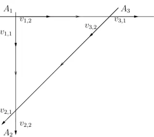
Consider the space C\{1, −1} and the coefficient system L on it that changes its sign under any loop based at 0 that passes once around 1 or −1. Let f be the map z 7→ −z and let ˜f : L → L be the map that covers f and is identical over 0.

(29)

24 CHAPTER 4. SOME FURTHER PRELIMINARIES i −i b i −i c Figure 4.1:

Proposition 4.1 The map ˜f acts on the groups H1(C \ {1, −1}, L), H1(C \

{1, −1}, L), and ¯H1(C \ {1, −1}, L) as the multiplication by −1.

♦

Consider B(C∗_{, 2), i.e. the space of pairs of points in C \ {0}. It is a fibre}

bundle over C∗_{, the projection p : B(C}∗_{, 2) → C}∗_{being just the multiplication.}

The fibre is homeomorphic to C \ {1, −1}, and the action of the generator of π1(C∗) is z 7→ −z. The fibre p−1(1) contracts to the character “8”. Denote by

b, c the loops in p−1_{(1) based at {±i} and represented schematically on Figure}

4.1; note that they correspond to the circles of the “8”. Denote by a the loop t 7→ {ieπit_{, −ie}πit_}.

Consider the following three local systems on B(C∗_{, 2) (the fibre of each of}

them is R):

1. A1 changes its sign under a and does not change its sign under b and c.

2. A2 changes its sign under b and c and does not change its sign under a.

3. A3 changes its sign under all loops a, b, c.

Note that we have A3= ±R.

Let f be the map B(C∗_{, 2) → B(C}∗_{, 2) induced by the map z 7→ 1/z and let}

fi_{: A}

i→ Ai, i = 1, 2, 3 be the map that covers f and is identical over the fibre

p−1_(1).

Proposition 4.2 1. ¯P (B(C∗_{, 2), A}₁_{) =} _{P (B(C}¯ ∗_{, 2), A}₃_{) = t}2_{(1 + t),}

¯

P (B(C∗_{, 2), A}₂_{) = 0 (recall that we denote by ¯}_{P the}

“Borel-Moore-Poincar´e” polynomial, see page 1). 2. The map fi

∗acts as the identity on ¯H3(B(C∗, 2), Ai) and as minus identity

(30)

4.2. SOME TECHNICAL LEMMAS 25 Note that the lifting of the generator of π1(C∗) is as follows: γ{a,b}(t) =

{aeπit_{, be}πit_{}, where {a, b} ∈ p}−1_(1).

(31)

Chapter 5

Smooth plane quintics

In this chapter we use the method described in chapter 3 to calculate the real cohomology groups of the space of polynomials that define smooth complex plane projective quintics. Recall that on page 1 we defined the spaces Πd,nand

Σd,n for any integers d, n ≥ 1.

Theorem 5.1 The Poincar´e polynomial of the space Π5,2\ Σ5,2 is equal to

(1 + t)(1 + t3)(1 + t5).

By the Alexander duality, the cohomology group of Π5,2\ Σ5,2is isomorphic

to the Borel-Moore homology of Σ5,2:

Hi(Π5,2\ Σ5,2, R) = ¯H2D−1−i(Σ5,2, R),

where D = dimC(Π5) = 21 and 0 < i < 2D − 1. This reduction was used first by

V. I. Arnold in [2]. To calculate the latter group ¯H_∗(Σ, R) we use the method constructed in chapter 3. It is described by the following theorem.

Theorem 5.2 There exists a spectral sequence that converges to the real Borel-Moore homology of the space Σ5,2 and is defined by the following conditions:

1. Any its nontrivial term E1

p,q belongs to the quadrilateral in the (p,

q)-plane, defined by the conditions [1 ≤ p ≤ 3, 29 ≤ q ≤ 39]. 2. In this quadrilateral all the nontrivial terms E1

p,q look as is shown in

(5.1).

3. The spectral sequence stabilises in this term, i.e. E1_{≡ E}∞_.

39 R 38 37 R 36 35 R R 34 33 R 32 31 R 30 29 R 1 2 3 (5.1) 26

Résolutions coniques des variétés discriminants e applications à la géométrie algébrique complexe et réelle

HAL Id: tel-00012101

https://tel.archives-ouvertes.fr/tel-00012101

Submitted on 9 Apr 2006

HAL is a multi-disciplinary open access

archive for the deposit and dissemination of

sci-entific research documents, whether they are

pub-lished or not. The documents may come from

teaching and research institutions in France or

abroad, or from public or private research centers.

L’archive ouverte pluridisciplinaire HAL, est

destinée au dépôt et à la diffusion de documents

scientifiques de niveau recherche, publiés ou non,

émanant des établissements d’enseignement et de

recherche français ou étrangers, des laboratoires

publics ou privés.

Résolutions coniques des variétés discriminants e

applications à la géométrie algébrique complexe et réelle

Alexey Gorinov

To cite this version:

Alexey Gorinov. Résolutions coniques des variétés discriminants e applications à la géométrie

al-gébrique complexe et réelle. Mathématiques [math]. Université Paris-Diderot - Paris VII, 2004.

Français. �tel-00012101�

UNIVERSIT ´

E PARIS 7 - DENIS DIDEROT

UFR de Math´

ematiques

Th`

ese

Pr´esent´ee pour obtenir le diplˆ

ome de

Docteur de l’Universit´

e Paris 7

Spécialité: Mathématiques

Pr´

esent´

ee et soutenue publiquement le vendredi 17 d´

ecembre 2004

par

Alexei Gorinov

R´

esolutions coniques des vari´

et´

es

discriminants et applications `

a la

g´

eom´

etrie alg´

ebrique complexe et r´

eelle

Directeur de th`

ese :

P. Vogel

Rapporteurs :

I. Itenberg

V. Vassiliev

Jury :

V. Kharlamov

S. Orevkov

C. Peters

J. Steenbrink

Contents

Some conventions and

notation

Acknoledgements

Chapter 1

Introduction

Chapter 2

Introduction

Chapter 3

The method of conical

resolutions

3.1

Why generalise?

3.2

The construction of the conical resolution

Chapter 4

Some further preliminaries

4.1