HAL Id: tel-01224747
https://tel.archives-ouvertes.fr/tel-01224747
Submitted on 5 Nov 2015HAL is a multi-disciplinary open access archive for the deposit and dissemination of sci-entific research documents, whether they are pub-lished or not. The documents may come from teaching and research institutions in France or abroad, or from public or private research centers.
L’archive ouverte pluridisciplinaire HAL, est destinée au dépôt et à la diffusion de documents scientifiques de niveau recherche, publiés ou non, émanant des établissements d’enseignement et de recherche français ou étrangers, des laboratoires publics ou privés.
Distributed under a Creative Commons Attribution - NonCommercial - NoDerivatives| 4.0
algorithms for sparse linear estimation problems in
signal processing and coding theory
Jean Barbier
To cite this version:
Jean Barbier. Statistical physics and approximate message passing algorithms for sparse linear esti-mation problems in signal processing and coding theory. Inforesti-mation Theory [math.IT]. Université Paris Diderot, 2015. English. �tel-01224747�
APPROXIMATE MESSAGE PASSING ALGORITHMS
FOR SPARSE LINEAR ESTIMATION PROBLEMS
IN SIGNAL PROCESSING AND CODING THEORY
Thèse n.
présentée le 18 septembre 2015 à l’École Normale Supérieure de Paris.
Travail effectué au laboratoire de physique statistique de l’École Normale Supérieure de Paris
sous la direction de Prof. Florent KRZAKALA
et au sein de l’école doctorale physique en île de France Université Paris Diderot (Paris 7) Sorbonne Paris cité pour l’obtention du grade de Docteur ès Sciences spécialité physique théorique, par
Jean BARBIER
acceptée sur la proposition du jury: Prof. Laurent DAUDET, examinateur Prof. Silvio FRANZ, examinateur Prof. Florent KRZAKALA, directeur Prof. Marc LELARGE, examinateur Prof. Nicolas MACRIS, rapporteur Prof. Marc MÉZARD, examinateur
Prof. Federico RICCI-TERSENGHI, examinateur Prof. David SAAD, rapporteur
A mes parents qui m’ont tout donné et mes soeurs que j’aime par dessus tout. Merci de m’avoir supporté jusqu’ici...
Je tiens avant tout à remercier mes parents qui m’ont toujours laissé totalement libre de mes choix et m’ont tout donné, qui m’ont soutenu pendant cette longue période souvent difficile, parfois très difficile et toujours merveilleuse qu’ont été mes études. Merci à mes soeurs, Louise et Virginie. Merci à toute ma famille, présente dans les joies et difficultés.
Je remercie mon directeur Florent, le maitre Jedi, un ami. Merci de m’avoir fait confiance, de m’avoir enseigné par la pratique le vrai sens critique, de m’avoir présenté tant de personnes incroyables, de m’avoir offert ces expériences enrichissantes en école et ailleurs, d’avoir été insupportable quand il le fallait vraiment et d’avoir toujours su trouver l’équilibre entre pression et liberté, travail et humour, entre aide et indépendance. Je n’aurais réellement pas pu vivre une meilleure expérience pour mon doctorat.
Merci à Eric Tramel et Francesco Caltagirone pour leur sympathie et leurs explications. Je tiens à remercier ceux qui ont rendu ma thèse encore plus agréable par leur amitié, qui ont transformé tous mes repas (et soirées) en moments toujours plus marrants, qui m’ont presentés leurs amis... Merci Thim, Thomas, le petit Christophe, Alaa, Alice, Antoine, Sophie, Ralph et merci à tous les autres aussi.
Je voudrais également remercier ceux qui m’ont permis d’en arriver là. En particulier Riccardo Zecchina qui m’a fait découvrir les domaines de l’inférence et de la belle physique statistique du désordre, Alessandro Pelizzola qui a tout fait pour rendre mon année à Turin si enrichissante et simple, Silvio Franz et Emmanuel Trizac pour m’avoir fait confiance en m’envoyant en Italie, merci à Marc Mézard pour son influence directe ou indirecte dans tous les travaux auxquels j’ai pu m’intéresser pendant ces trois années et demie, sur tous les papiers que j’ai pu lire et pour m’avoir montré ce que c’est que de vraiment savoir skier... Merci à Lenka Zdeborova pour ces collaborations fructueuses, Laurent Daudet pour m’avoir aidé à prendre des décisions importantes.
Merci aussi à Rüdiger Urbanke et Nicolas Macris pour leur accueil à Lausanne. J’attends avec impatience les années à venir... Merci aux autres membres de mon jury de prendre le temps pour ma soutenance et avoir la patience de lire ma thèse: David Saad, Federico Ricci-Tersenghi et Marc Lelarge.
Je n’oublie pas les membres de mon premier lieu de travail, le laboratoire de physico-chimie théorique de l’École Supérieure de physique et chimie de Paris, en particulier Élie Raphaël et Thomas Salez pour leur sympathie perpétuelle, ainsi que Justine et Antoine.
Je dois beaucoup à mes colocataires qui m’auront supporté malgré mes crises de nerfs suite à trop de message-passing et avec qui j’aurais tellement rigolé: Charlotte, PH et Manon, vous
êtes les meilleurs.
Merci Auré d’avoir rendu mes études encore plus intéressantes, du début à la fin.
Je n’oublie pas Brian et tous les serveurs de Chez Léa sans qui cette période de rédaction aurait été très différente...
Je tiens également à remercier la DGA de m’avoir financé.
La liste pourrait encore continuer longtemps ayant rencontré tellement de gens intéressants et sympathiques durant ces années, merci à vous tous..
This thesis is interested in the application of statistical physics methods and inference to signal processing and coding theory, more precisely, to sparse linear estimation problems.
The main tools are essentially the graphical models and the approximate message-passing algorithm together with the cavity method (referred as the state evolution analysis in the signal processing context) for its theoretical analysis. We will also use the replica method of statistical physics of disordered systems which allows to associate to the studied problems a cost function referred as the potential of free entropy in physics. It allows to predict the different phases of typical complexity of the problem as a function of external parameters such as the noise level or the number of measurements one has about the signal: the inference can be typically easy, hard or impossible. We will see that the hard phase corresponds to a regime of coexistence of the actual solution together with another unwanted solution of the message passing equations. In this phase, it represents a metastable state which is not the true equilibrium solution. This phenomenon can be linked to supercooled water blocked in the liquid state below its freezing critical temperature.
Thanks to this understanding of blocking phenomenon of the algorithm, we will use a method that allows to overcome the metastability mimicing the strategy adopted by nature itself for supercooled water: the nucleation and spatial coupling. In supercooled water, a weak localized perturbation is enough to create a crystal nucleus that will propagate in all the medium thanks to the physical couplings between closeby atoms. The same process will help the algorithm to find the signal, thanks to the introduction of a nucleus containing local information about the signal. It will then spread as a "reconstruction wave" similar to the crystal in the water. After an introduction to statistical inference and sparse linear estimation, we will introduce the necessary tools. Then we will move to applications of these notions. They will be divided into two parts.
The signal processing part will focus essentially on the compressed sensing problem where we seek to infer a sparse signal from a small number of linear projections of it that can be noisy. We will study in details the influence of structured operators instead of purely random ones used originally in compressed sensing. These allow a substantial gain in computational complexity and necessary memory allocation, which are necessary conditions in order to work with very large signals. We will see that the combined use of such operators with spatial coupling allows the implementation of an highly optimized algorithm able to reach near to optimal performances. We will also study the algorithm behavior for reconstruction of
approximately sparse signals, a fundamental question for the application of compressed sensing to real life problems. A direct application will be studied via the reconstruction of images measured by fluorescence microscopy. The reconstruction of "natural" images will be considered as well.
In coding theory, we will look at the message-passing decoding performances for two distincts real noisy channel models. A first scheme where the signal to infer will be the noise itself will be presented. The second one, the sparse superposition codes for the additive white Gaussian noise channel is the first example of error correction scheme directly interpreted as a structured compressed sensing problem. Here we will apply all the tools developed in this thesis for finally obtaining a very promising decoder that allows to decode at very high transmission rates, very close of the fundamental channel limit.
Keywords: Statistical physics, disordered systems, mean field theory, signal processing, Bayesian inference, statistical learning, coding theory, linear estimation, sparsity, approx-imate sparsity, compressed sensing, spatial coupling, Gaussian channel, error correcting codes, sparse superposition codes, approximate message passing algorithm, cavity method, state evolution analysis, replica method.
Cette thèse s’intéresse à l’application de méthodes de physique statistique des systèmes désordonnés ainsi que de l’inférence à des problèmes issus du traitement du signal et de la théorie du codage, plus précisément, aux problèmes parcimonieux d’estimation linéaire. Les outils utilisés sont essentiellement les modèles graphiques et l’algorithme approximé de passage de messages ainsi que la méthode de la cavité (appelée analyse de l’évolution d’état dans le contexte du traitement de signal) pour son analyse théorique. Nous aurons également recours à la méthode des répliques de la physique des systèmes désordonnées qui permet d’associer aux problèmes rencontrés une fonction de coût appelé potentiel ou entropie libre en physique. Celle-ci permettra de prédire les différentes phases de complexité typique du problème, en fonction de paramètres externes tels que le niveau de bruit ou le nombre de mesures liées au signal auquel l’on a accès : l’inférence pourra être ainsi typiquement simple, possible mais difficile et enfin impossible. Nous verrons que la phase difficile correspond à un régime où coexistent la solution recherchée ainsi qu’une autre solution des équations de passage de messages. Dans cette phase, celle-ci est un état métastable et ne représente donc pas l’équilibre thermodynamique. Ce phénomène peut-être rapproché de la surfusion de l’eau, bloquée dans l’état liquide à une température où elle devrait être solide pour être à l’équilibre.
Via cette compréhension du phénomène de blocage de l’algorithme, nous utiliserons une méthode permettant de franchir l’état métastable en imitant la stratégie adoptée par la nature pour la surfusion : la nucléation et le couplage spatial. Dans de l’eau en état métastable liquide, il suffit d’une légère perturbation localisée pour que se créer un noyau de cristal qui va rapidement se propager dans tout le système de proche en proche grâce aux couplages physiques entre atomes. Le même procédé sera utilisé pour aider l’algorithme à retrouver le signal, et ce grâce à l’introduction d’un noyau contenant de l’information locale sur le signal. Celui-ci se propagera ensuite via une "onde de reconstruction" similaire à la propagation de proche en proche du cristal dans l’eau.
Après une introduction à l’inférence statistique et aux problèmes d’estimation linéaires, on introduira les outils nécessaires. Seront ensuite présentées des applications de ces notions. Celles-ci seront divisées en deux parties.
La partie traitement du signal se concentre essentiellement sur le problème de l’acquisition comprimée où l’on cherche à inférer un signal parcimonieux dont on connaît un nombre restreint de projections linéaires qui peuvent être bruitées. Est étudiée en profondeur
l’in-fluence de l’utilisation d’opérateurs structurés à la place des matrices aléatoires utilisées originellement en acquisition comprimée. Ceux-ci permettent un gain substantiel en temps de traitement et en allocation de mémoire, conditions nécessaires pour le traitement algo-rithmique de très grands signaux. Nous verrons que l’utilisation combinée de tels opérateurs avec la méthode du couplage spatial permet d’obtenir un algorithme de reconstruction extrê-mement optimisé et s’approchant des performances optimales. Nous étudierons également le comportement de l’algorithme confronté à des signaux seulement approximativement parcimonieux, question fondamentale pour l’application concrète de l’acquisition compri-mée sur des signaux physiques réels. Une application directe sera étudiée au travers de la reconstruction d’images mesurées par microscopie à fluorescence. La reconstruction d’images dites "naturelles" sera également étudiée.
En théorie du codage, seront étudiées les performances du décodeur basé sur le passage de message pour deux modèles distincts de canaux continus. Nous étudierons un schéma où le signal inféré sera en fait le bruit que l’on pourra ainsi soustraire au signal reçu. Le second, les codes de superposition parcimonieuse pour le canal additif Gaussien est le premier exemple de schéma de codes correcteurs d’erreurs pouvant être directement interprété comme un problème d’acquisition comprimée structuré. Dans ce schéma, nous appliquerons une grande partie des techniques étudiée dans cette thèse pour finalement obtenir un décodeur ayant des résultats très prometteurs à des taux d’information transmise extrêmement proches de la limite théorique de transmission du canal.
Mots clefs : Physique statistique, systèmes désordonnés, théorie du champ moyen, traitement du signal, inférence Bayesienne, apprentissage statistique, théorie du codage, estimation linéaire, parcimonie, parcimonie approximative, acquisition comprimée, couplage spatial, canal Gaussien, codes correcteurs d’erreurs, codes de superposition parcimonieuse, algo-rithme approximé de passage de messages, méthode de la cavité, analyse d’évolution des états, méthode des répliques.
Remerciements v
Abstract (English/Français) vii
List of figures xvi
List of symbols and acronyms xix
I Main contributions and structure of the thesis 1
1 Main contributions 3
1.1 Combinatorial optimization . . . 3 1.1.1 Study of the independent set problem, or hard core model on random
regular graphs by the one step replica symmetry breaking cavity method 3 1.2 Signal processing and compressed sensing . . . 4
1.2.1 Generic expectation maximization approximate message-passing solver for compressed sensing . . . 4 1.2.2 Approximate message-passing for approximate sparsity in compressed
sensing . . . 4 1.2.3 Influence of structured operators with approximate message-passing for
the compressed sensing of real and complex signals . . . 5 1.2.4 "Total variation" like reconstruction of natural images by approximate
message-passing . . . 5 1.2.5 Compressive fluorescence microscopy images reconstruction with
ap-proximate message-passing . . . 5 1.3 Coding theory for real channels . . . 6
1.3.1 Error correction of real signals corrupted by an approximately sparse Gaussian noise . . . 6 1.3.2 Study of the approximate message-passing decoder for sparse
superposi-tion codes over the additive white Gaussian noise channel . . . 6
II Fundamental concepts and tools 11 3 Statistical inference and linear estimation problems for the physicist layman 13
3.1 What is statistical inference ? . . . 14
3.1.1 General formulation of a statistical inference problem . . . 14
3.1.2 Inverse versus direct problems . . . 15
3.1.3 Estimation versus prediction . . . 16
3.1.4 Supervised versus unsupervised inference . . . 17
3.1.5 Parametric versus non parametric inference . . . 18
3.1.6 The bias-variance tradeoff: what a good estimator is ? . . . 19
3.1.7 Another source of error: the finite size effects . . . 22
3.1.8 Some important parametric supervised inference problems . . . 23
3.2 Linear estimation problems and compressed sensing . . . 24
3.2.1 Approximate fitting versus inference . . . 25
3.2.2 Sparsity and compressed sensing . . . 26
3.2.3 Why is compressed sensing so useful? . . . 28
3.3 The tradeoff between statistical and computationnal efficiency . . . 30
3.3.1 A quick detour in complexity theory and worst case analysis : P 6= NP ? . 30 3.3.2 Complexity of sparse linear estimation and notion of typical complexity 31 3.4 The convex optimization approach . . . 32
3.4.1 The LASSO regression for sparse linear estimation . . . 32
3.4.2 Why is the`1norm a good norm ? . . . 33
3.4.3 Advantages and disadvantages of convex optimization . . . 34
3.5 The basics of information theory . . . 35
3.5.1 Incertitude and information: the entropy . . . 35
3.5.2 The mutual information . . . 37
3.5.3 The Kullback-Leibler divergence . . . 38
3.6 The Bayesian inference approach . . . 39
3.6.1 The method applied to compressed sensing . . . 39
3.6.2 Different estimators for minimizing different risks: Bayesian decision theory . . . 41
3.6.3 Why is the minimum mean square error estimator the more appropriate ? A physics point of view . . . 43
3.6.4 Solving convex optimization problems with Bayesian inference . . . 46
3.7 Error correction over the additive white Gaussian noise channel . . . 46
3.7.1 The power constrained additive white Gaussian noise channel and its capacity . . . 47
3.7.2 Linear coding and the decoding problem . . . 50
4 Mean field theory, graphical models and message-passing algorithms 53 4.1 Bayesian inference as an optimization problem and graphical models . . . 54
4.1.1 The variational method and Gibbs free energy . . . 54
4.1.3 Justification of mean field approximations by maximum entropy criterion 56
4.1.4 The maximum entropy criterion finds the most probable model . . . 58
4.1.5 Factor graphs . . . 58
4.1.6 The Hamiltonian of linear estimation problems and compressed sensing 59 4.1.7 Naive mean field estimation for compressed sensing . . . 60
4.2 Belief propagation and cavities . . . 63
4.2.1 The canonical belief propagation equations . . . 63
4.2.2 Understanding belief propagation in terms of cavity graphs . . . 64
4.2.3 Derivation of belief propagation from cavities and the assumption of Bethe measure . . . 65
4.2.4 When does belief propagation work . . . 67
4.2.5 Belief propagation and the Bethe free energy . . . 68
4.2.6 The Bethe free energy in terms of cavity messages . . . 70
4.2.7 Derivation of belief propagation from the Bethe free energy . . . 71
4.3 The approximate message-passing algorithm . . . 72
4.3.1 Why is the canonical belief propagation not an option for dense linear systems over reals? . . . 73
4.3.2 Why message-passing works on dense graphs? . . . 75
4.3.3 Derivation of the approximate message-passing algorithm from belief propagation . . . 76
4.3.4 Alternative "simpler" derivation of the approximate message-passing algorithm . . . 83
4.3.5 Understanding the approximate message-passing algorithm . . . 86
4.3.6 How to quickly cook an approximate message-passing algorithm for your linear estimation problem . . . 86
4.3.7 The Bethe free energy for large dense graphs with i.i.d additive white Gaussian noise . . . 88
4.3.8 Learning of the model parameters by expectation maximization . . . 94
4.3.9 Dealing with non zero mean measurement matrices . . . 95
5 Phase transitions, asymptotic analyzes and spatial coupling 97 5.1 Disorder and typical complexity phase transitions in linear estimation . . . 98
5.1.1 Typical phase diagram in sparse linear estimation and the nature of the phase transitions . . . 98
5.2 The replica method for linear estimation over the additive white Gaussian noise channel . . . 104
5.2.1 Replica trick and replicated partition function . . . 105
5.2.2 Saddle point estimation . . . 110
5.2.3 The prior matching condition . . . 110
5.3 The cavity method for linear estimation: state evolution analysis . . . 111
5.3.1 Derivation starting from the approximate message-passing algorithm . 112 5.3.2 Alternative derivation starting from the cavity quantities . . . 115
5.3.3 The prior matching condition and Bayesian optimality . . . 116
5.4 The link between replica and state evolution analyzes: derivation of the state evolution from the average Bethe free entropy . . . 120
5.4.1 Different forms of the Bethe free entropy for different fixed points algo-rithms . . . 121
5.5 Spatial coupling for optimal inference in linear estimation . . . 122
5.5.1 The spatially-coupled operator and the reconstruction wave propagation 123 5.6 The spatially-coupled approximate message-passing algorithm . . . 125
5.6.1 Further simplifications for random matrices with zero mean and equiva-lence with Montanari’s notations . . . 126
5.7 State evolution analysis in the spatially-coupled measurement operator case . 129 III Signal processing 135 6 Compressed sensing of approximately sparse signals 137 6.1 The bi-Gaussian prior for approximate sparsity . . . 138
6.1.1 Learning of the prior model parameters . . . 139
6.2 Reconstruction of approximately sparse signals with the approximate message-passing algorithm . . . 139
6.2.1 State evolution of the algorithm with homogeneous measurement matrices140 6.2.2 Study of the optimal reconstruction limit by the replica method . . . 140
6.3 Phase diagrams for compressed sensing of approximately sparse signals . . . . 143
6.4 Reconstruction of approximately sparse signals with optimality achieving matrices146 6.4.1 Restoring optimality thanks to spatial coupling . . . 147
6.4.2 Finite size effects influence on spatial coupling performances . . . 150
6.5 Some results on real images . . . 150
6.6 Concluding remarks . . . 153
7 Approximate message-passing with spatially-coupled structured operators 157 7.1 Problem setting . . . 158
7.1.1 Spatially-coupled structured measurement operators . . . 159
7.1.2 The approximate message-passing algorithm for complex signals . . . . 159
7.1.3 Randomization of the structured operators . . . 161
7.2 Results for noiseless compressed sensing . . . 162
7.2.1 Homogeneous structured operators . . . 166
7.2.2 Spatially-coupled structured operators . . . 166
7.3 Conclusion . . . 166
8 Approximate message-passing for compressive imaging 169 8.1 Reconstruction of natural images in the compressive regime by "total-variation-minimization"-like approximate message-passing . . . 169
8.1.1 Proposed model . . . 170
8.1.3 The learning equations . . . 173
8.1.4 Numerical experiments . . . 174
8.1.5 Concluding remarks . . . 175
8.2 Image reconstruction in compressive fluorescence microscopy . . . 187
8.2.1 Introduction . . . 187
8.2.2 Experimental setup and algorithmic setting . . . 188
8.2.3 A proposal of denoisers for the reconstruction of point-like objects mea-sured by compressive fluorescence microscopy . . . 191
8.2.4 Optimal Bayesian decision for the beads locations . . . 191
8.2.5 The learning equations . . . 192
8.2.6 Improvement using small first neighbor mean field interactions between pixels . . . 193
8.2.7 Reconstruction results on experimental data . . . 194
8.2.8 Concluding remarks and open questions . . . 194
IV Coding theory 199 9 Approximate message-passing decoder and capacity-achieving sparse superposition codes 201 9.1 Introduction . . . 201
9.1.1 Related works . . . 202
9.1.2 Main contributions of the present study . . . 203
9.2 Sparse superposition codes . . . 204
9.3 Approximate message-passing decoder for superposition codes . . . 208
9.3.1 The fast Hadamard-based coding operator . . . 208
9.4 State evolution analysis for random i.i.d homogeneous operators with constant power allocation . . . 209
9.5 State evolution analysis for spatially-coupled i.i.d operators or with power allo-cation . . . 213
9.5.1 State evolution for power allocated signals . . . 213
9.6 Replica analysis and phase diagram . . . 216
9.6.1 Large section limit of the superposition codes by analogy with the random energy model . . . 218
9.6.2 Alternative derivation of the large section limit via the replica method . 221 9.6.3 Results from the replica analysis . . . 225
9.7 Optimality of the approximate message-passing decoder with a proper power allocation . . . 230
9.8 Numerical experiments for finite size signals . . . 232
10 Robust error correction for real-valued signals via message-passing decoding and
spatial coupling 239
10.1 Introduction . . . 239
10.2 Compressed sensing based error correction . . . 240
10.2.1 Performance of the approximate message-passing decoder . . . 241
10.3 Numerical tests and finite size study . . . 243
10.4 Discussion . . . 245
3.1 Relations between the statistical physics quantities and vocabulary with the
inference and signal processing one . . . 17
3.2 The bias-variance tradeoff . . . 21
3.3 Geometrical interpretation of`1and`2norms . . . 34
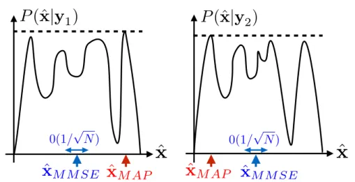
3.4 Minimum mean square error and maximum-a-posteriori estimators . . . 44
3.5 Posterior with a mode given by a very rare event . . . 45
3.6 Generic noisy channel in the probabilistic framework . . . 47
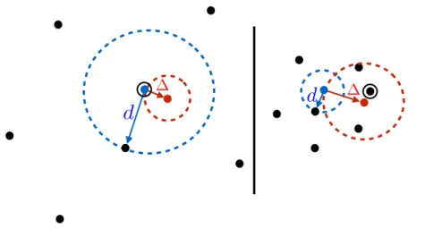
3.7 Reliable and unreliable codebooks . . . 51
4.1 Factor graph of linear estimation problems under i.i.d AWGN corruption . . . 59
4.2 The mean field algorithm for compressed sensing . . . 62
4.3 The belief propagation equations in terms of cavity graphs . . . 64
4.4 A cavity graph extension . . . 66
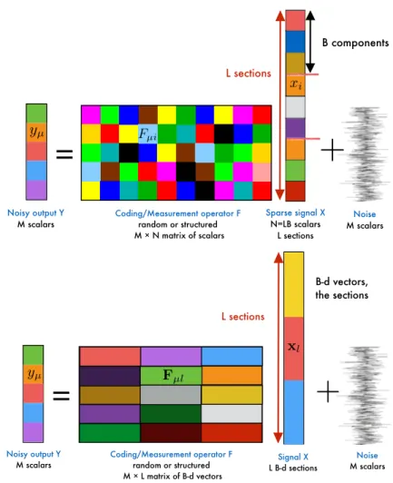
4.5 Equivalence between the compressed sensing of prior-correlated scalar signals and i.i.d vectorial components signals . . . 74
4.6 Generic approximate message-passing algorithm with damping . . . 83
4.7 Graphical representation of the approximate message-passing algorithm . . . 85
5.1 Typical phase diagram in sparse linear estimation under sparsity assumption 100 5.2 Bethe free entropy shape in the different typical complexity phases . . . 101
5.3 Bethe free entropy at the different transitions . . . 102
5.4 Spatial coupling in sparse linear estimation and the reconstruction wave prop-agation . . . 124
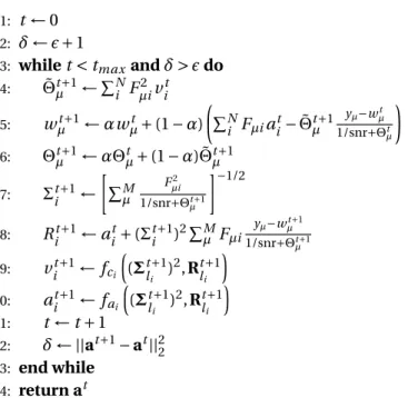
5.5 The AMP algorithm written with operators . . . 126
5.6 Simplified full-TAP version of the AMP algorithm with operators . . . 127
6.1 State evolution for approximately sparse signals . . . 141
6.2 Bethe free entropy for compressed sensing of approximately sparse signals at the phase transitions points . . . 142
6.3 From a first order to a continuous transition in compressed sensing with ap-proximate sparsity . . . 144
6.4 Appearance of the BP transition as the small components variance is decreased and comparison of the AMP reconstruction performances with the Bayes opti-mal inference . . . 145
6.5 Phase diagram for compressed sensing of approximately sparse signals in the
(²,α) plane . . . 146
6.6 Phase diagrams for compressed sensing of approximately sparse signals in the (α,ρ) plane for different small components variances . . . 147
6.7 State evolution for approximate sparsity with spatially-coupled matrices and comparison with the AMP results on finite size signals . . . 148
6.8 Asymptotic convergence time required by AMP for reconstructing approxi-mately sparse signals . . . 149
6.9 Fraction of instances reconstructed with spatially-coupled matrices . . . 151
6.10 Phase diagram with finite size instances solved by spatial coupling . . . 152
6.11 Sorted wavelet spectrum of the 4-steps Haar transformed Lena and peppers images . . . 153
6.12 Reconstruction results of Lena using approximate sparsity in the Haar wavelet basis . . . 154
6.13 Reconstruction results of the peppers image using approximate sparsity in the Haar wavelet basis . . . 155
7.1 spatially-coupled structured operator . . . 158
7.2 Complex AMP algorithm with operators . . . 161
7.3 Phase diagram of noiseless compressed sensing of real and complex signals, with instances solved with structured operators . . . 163
7.4 State evolution for spatially-coupled operators and comparison with structured operators . . . 164
7.5 Comparison of the running time with fast operators and random ones . . . . 165
8.1 The pixel i with its four closest neighbors . . . 171
8.2 Images used for the TV-reconstruction comparisons . . . 176
8.3 Comparison of the final reconstruction results for Lena . . . 177
8.4 Comparison of the final reconstruction results for Barbara . . . 179
8.5 Comparison of the final reconstruction results for Baboon . . . 181
8.6 Comparison of the final reconstruction results for Cameraman . . . 183
8.7 Comparison of the final reconstruction results for Peppers . . . 185
8.8 Experimental setup for compressive fluorescence microscopy measurements 187 8.9 Typical bi-dimensional Hadamard pattern used for the compressive measure-ments of the fluorescent beads . . . 189
8.10 Comparison of the beads location at M = 8192 . . . 196
8.11 Comparison of the beads location at M = 4096 . . . 196
8.12 Comparison of the beads location at M = 2048 . . . 197
8.13 Comparison of the beads location at M = 1024 . . . 197
8.14 Comparison of the beads location at M = 512 . . . 198
8.15 Comparison of the beads location at M = 400 . . . 198
9.2 Estimation problem associated to the decoding of the sparse signal over the AWGN channel and equivalence between the scalar and vectorial interpreta-tions of the signal components . . . 206 9.3 Factor graph associated to the sparse superposition codes . . . 207 9.4 Convergence of structured operators performances to the random operator ones209 9.5 State evolution and decoder performances with homogeneous matrices at
snr = 15 . . . 210 9.6 State evolution and decoder performances with homogeneous matrices at
snr = 7/100 . . . 211 9.7 State evolution for spatially-coupled superposition codes . . . 214 9.8 Equivalence between non constant power allocation and a particular strutured
operator . . . 215 9.9 Bethe free entropy for sparse superposition codes at the different transitions . 216 9.10 Phase diagrams of superposition codes at various snr . . . 226 9.11 Convergence rate of the optimal transition of superposition codes to the
ca-pacity and of the BP transition to its asymptotic value . . . 227 9.12 Optimal section error rate as a function of the section size and the snr . . . 228 9.13 Optimal section error rate for superposition codes in the (R, B ) plane . . . 229 9.14 Block and section error rates and finite size effects for superposition codes . . 233 9.15 Phase diagram of superposition codes with finite size results . . . 235 9.16 Comparison between power allocation and spatial coupling . . . 237
10.1 Phase diagram for error correction of real-valued signals corrupted by approxi-mately sparse Gaussian noise . . . 242 10.2 Robustness to noise of the error correction of real-valued signals corrupted by
an approximately sparse Gaussian channel . . . 244 10.3 Success rates of decoding with AMP over the approximately sparse Gaussian
channel . . . 246 10.4 Decoding Lena corrupted by the approximately sparse Gaussian noise channel 246
a : a generic quantity, usually a scalar if not precised further. a : a vector.
A : a matrix.
ai= (a)i : the it hcomponent of a. The two notations are equivalent.
Ai j : the element at the it hline and jt hcolumn of A.
Ai ,• : the it hline of A. A•,i : the it hcolumn of A.
s : generally the signal or message to infer. x : an intermediate variable for estimating s. ˆx : the final estimate of the signal s.
y : the measurement vector or codeword. F : the measurement or coding operator.
ˆ
a : the estimate of the quantity a.
K : number of non zero components in the sparse signal s.
N : number of scalar components of the signal or message to reconstruct s.
L : number of vector components of the signal or message to reconstruct s.
M : number of scalar components of the measure or codeword y. := : equal by definition.
ρ := K /N : density of non zero components of s. α := M/N : the measurement rate.
a|b : a "given" (or such that) b.
N (u|µ,σ2) : a Gaussian distribution for the random variable u
with meanµ and variance σ2.
δ(x) : the delta Dirac function (which is formally a distribution)
that is a probability density giving a infinite weight to the single value x = 0.
δi j : the kronecker symbol, which is one if i = j , 0 else.
∂i := {j : (i j) ∈ E} : the set of neighbors nodes to node i in the
graphical representation of the problem (E is the set of edges).
∂i\j : the set of neighbors nodes to node i except the node j
in the graphical representation of the problem.
u ∼ P(u|θ) : u is a random variable with distribution P(u|θ)
that depends on a vector of parametersθ.
Ex(y(x)) = EP(y(x)) : the average of the function y(x) with respect to the random
variable x ∼ P(x). The two notations are used equivalently when there are no possible ambiguities.
< x >:= 1/N
N
X
i
xi : the empirical average of the vector x (here there are N components).
©xi| f (xi)
ªb
g (i ) : the ensemble made of {xi} that verify the conditions
f (xi) ∀ i ∈ {1,...,b|g (i ) is true}.
As for any operations such as sums, products, etc,
if the lower bound of the index is not explicited, it means it starts from 1.
For example, {ai|ai> 0}iN= {ai|ai> 0}Ni =1, N X i xi= N X i =1 xi, etc.
£xi| f (xi)¤bg (i ) : the concatenation of©xi| f (xi)ªbg (i )to form a vector
of cardinality that depends on g and b.
[a, b] : the simple concatenation of a and b to form a vector.
I(E) : the indicator function, which is 1 if the condition E is true, 0 else. ∆ : the variance of the i.i.d Gaussian measurement noise.
ξ := £ξµ∼ N (ξµ|0, ∆)¤µM : the i.i.d Gaussian measurement noise vector.
||y||p:= 1/M µM X i |yi|p ¶1/p
: the rescaled`pnorm of y, which is here of size M .
snr := ||y||22/∆ : the signal to noise ratio, where y is the codeword.
z ∈ O(u) : z is a quantity of the same order as u i.e. z = Cu
z ∈ o(u) : z is a quantity at least an order smaller than u i.e. limz
u = 0
in a proper limit that depends on the context.
a ≈ b : a and b are equal up to a negligible difference ∈ o(a).
x\i:=£xj¤Nj 6=i : the vector made of the N − 1 components
of x that are not the it hone.
xa\i:=£xj∈ ∂a¤j 6=i : the vector of components of x that are neighbors
of the factor a, except the it hone.
d x :=
N
Y
i
d xi : integration over all the components of the size N vector x.
Dx :=YN i Dxi= N Y i
d xiN (xi|0, 1) : integration over all the components of the size N vector x
with unit centered Gaussian measure. X| : the transpose of a vector or matrix. xa:=£xa
i
¤N
i : the component wise power operation for a vector (or matrix).
XY := Z where Zi j= Xi jYi j : the component wise product between matrices
or vectors of same size.
x|y = xy|:=
N
X
i
xiyi : the scalar product between two vectors of size N .
The two notations are equivalent as we always assume the vectors to have proper dimensions to apply the product.
Fx :=£
N
X
i
Fµixi¤Mµ : the matrix product between F of size M × N and x of size N .
(Fx)µ:=
N
X
i
Fµixi : theµt hcomponent of the vector Fx.
VarP(u) := EP(u2) − EP(u)2 : the variance of the random variable u with distribution P .
inv (A) : the inverse of the matrix A.
∂x : the partial derivative with respect to x.
|x| : the number of components of x or the cardinality of an ensemble.
CS : compressed sensing. MSE : mean squarre error.
MMSE : minimum mean squarre error. MAP : maximum à posteriori.
i.e. : id est.
N -d : N -dimensional.
BP : belief propagation.
AMP : approximate message passing. SE : state evolution analysis.
i.i.d : independent and identically distributed. AWGN : additive white Gaussian noise.
My work has been concentrated around two main axis: i) signal processing through com-pressed sensing and its application in image reconstructions and ii) coding theory over real channels and its links to compressed sensing. I will present here my main contributions in these fields, dividing my work into practical achievements through algorithms design and the theoretical and asymptotic studies. In addition, I’ve worked on a combinatorial optimization problem, namely the independent set problem, in order to get familiar with the cavity method and the diverse phase transitions that occur in such problems. I will start by briefly present this piece of work that I won’t detail in this thesis. This choice has been made for sake of coherence of the thesis: all the problems I’ve worked on, except this one, belong to the class of sparse linear estimation problems and a common methodology is used, based on the approximate message-passing algorithm and the state evolution and replica analyzes for the asymptotic studies.
1.1 Combinatorial optimization
1.1.1 Study of the independent set problem, or hard core model on random regu-lar graphs by the one step replica symmetry breaking cavity method
In this work [1], we have studied the NP-hard independent set problem on random regular graphs, the dual of the vertex cover problem better known as the hard-core model in the physics literature. This model is of great interest as it can be seen as a lattice version of the hard spheres, a fundamental model in physics. The aim of this theoretical work was to reconciliate the two extreme regimes corresponding to the high and low connectivities of the graph. Both were known for a long time but each with a totally different behavior. While in the low connectivity regime, the problem displays a continuous full replica symmetry breaking transition as the density of particles increases in the graph, it was proven in the mathematical literature that in the high connectivity limit, the opposite phenomenon happens: the space of solution breaks discontinuously into exponentially many well separated components, a behavior typically found in glassy systems, at a density which is the half of the maximum one.
The main result obtained through the cavity method is the obtention of the full phase diagram of the problem for all connectivities. The computation of the different phase transitions in the problem by population dynamics in the 1RSB framework shows that the change in behavior between a continuous full RSB regime and the appearance of the discontinuous 1RSB transition happens at connectivity K = 16. It appears that between 16 ≤ K < 20, despite the existence of a stable 1RSB glassy phase, the continous transition remains if the density of particles is too high until for K ≥ 20, the 1RSB phase becomes stable for all densities until the maximum one. This shows that this model is the simplest mean field model of the glass and jamming transitions, and can be used to get insights on more complex models such as the hard spheres in high dimensions. In addition, the asymptotic analysis in the cavity framework is in perfect agreement with the rigorous results at high connectivity, which supports further the validity of the cavity method in such problems despite it is not yet rigorously established.
1.2 Signal processing and compressed sensing
1.2.1 Generic expectation maximization approximate message-passing solver for compressed sensing
Practical achievements : I’ve implemented a modular AMP solver for compressed sensing in MATLAB, that includes a lot of different possible priors for the signal model. In addition, most of the free parameters in these priors and the noise variance can be learned efficiently through expectation maximisation. All the algorithms can be found athttps://github.com/ jeanbarbier/BPCS_common.
1.2.2 Approximate message-passing for approximate sparsity in compressed sens-ing
Practical achievements : My first work [2] during this thesis was focused on the study of the AMP performances and behavior when dealing with signals that are only approximately sparse, sometimes referred as compressible. We implemented a specifically designed prior for approximate sparsity, and the expectation maximisation learning of all the parameters of this prior.
Theoretical results : We performed the static and dynamical asymptotic analyzes thanks to the replica and state evolution techniques respectively. We extracted how the AMP performances change as a function of the variance of the small components part of the signal, a kind of effective noise, and what are the best possible results from the Bayesian point of view. A first order phase transition blocking the AMP solver under some measurement ratio appears, but we have shown how the spatial coupling strategy can restore the optimality of the AMP solver and until which level of effective noise it makes sense to use this strategy.
1.2.3 Influence of structured operators with approximate message-passing for the compressed sensing of real and complex signals
Practical achievements : A large amount of work has been put into the combination of this AMP solver with structured operators, based of fast Hadamard and Fourier transforms [3]. Furthermore, I’ve developed a set of routines for applying the spatial coupling strategy in combination with these structured operators. The result is a very fast AMP solver yet optimal from the information theoretic point of view. It is able to deal with very large signals as the use of such operators allows to side step the memory issues that quickly arise working with the large matrices that one must store if not structured.
Theoretical results : Side to side with the developement of the AMP solver combined with full or spatially-coupled structured operators, we have studied how the use of such operators influence the performances of AMP in noiseless compressed sensing of real or complex signals. The point is that AMP together with the state evolution analysis has originally been derived for i.i.d matrices but we have numerically shown that despite the state evolution does not describe properly the AMP dynamic with structured operators, it remains an accurate predictive tool for its final performances as the reconstruction quality is the same than with i.i.d matrices. Furthermore, it appeared that structured operators improves the rate of convergence of AMP. In addition, the study of the spatial coupling strategy have shown that it performs very well with such operators as well and allows to make optimal inference as long as the signal density is not too large.
1.2.4 "Total variation" like reconstruction of natural images by approximate message-passing
Practical achievements : In order to reconstruct "natural images" (i.e. that are sparse in the discrete gradient space) in the compressive regime, I’ve worked on an AMP implementation mimicing the total-variation optimization algorithms. The result is an algorithm able to compete with the best optimization solvers in terms of reconstruction results, but with fewer parameters to tune as most of them can be learned efficiently.
1.2.5 Compressive fluorescence microscopy images reconstruction with approxi-mate message-passing
Practical achievements : Still in the field of compressive imaging, I’ve developed an AMP implementation for reconstruction of images measured by compressive fluorescence mi-croscopy, based on an approximate sparsity prior. The images here are highly sparse in the direct pixel space. The AMP overcomes the`1optimization solvers in terms of reconstruction
quality, speed and minimum undersampling ratio to get good results. Furthermore, all the free parameters of the model can be learned efficiently.
1.3 Coding theory for real channels
1.3.1 Error correction of real signals corrupted by an approximately sparse Gaus-sian noise
Practical achievements : My first introduction to the field of coding theory is through a work [4] that naturally followed the study of approximate sparsity in compressed sensing. In this work, the aim is error correction over a channel that adds to a real transmitted message an approximately sparse Gaussian noise with some large components, the others being a smaller amplitude background noise. The aim is the reconstruction of the noise in order to cancel it at the end. We naturally used our previously developed AMP solver for approximately sparse signals to design an efficient decoder. In addition, the use of spatial coupling in this context allowed the decoder to perform at high rate, well above the results obtained with previously developed convex optimization based solvers.
Theoretical results : Based on the state evolution analysis for compressed sensing of approxi-mately sparse signals, we predicted the asymptotic performances of our AMP based decoder, which shows that it is robust to the background noise, in the sense that the reconstruction error grows continuously with the variance of the small components of the noise.
1.3.2 Study of the approximate message-passing decoder for sparse superposi-tion codes over the additive white Gaussian noise channel
Practical achievements : We presented the first decoder based on AMP for the sparse su-perposition codes, a capacity achieving error correction scheme over the AWGN channel. We exposed the first close connection between the compressed sensing theory and error correcting codes, as the sparse superposition codes decoding can directly be interpreted as a compressed sensing problem for signals with structured sparsity, or equivalently of signals with vectorial components instead of scalar ones, for which compressed sensing has originally been developed.
Our first paper [5] on this topic studied the decoder when the coding matrix is i.i.d Gaussian and the power allocation of the transmitted message is constant. Despite the presence of a first order phase transition blocking the AMP decoder well before the capacity, the numerical results have shown that the perfomances are overcoming a previous decoder based on soft thresholding methods, the adaptative successive decoder. This decoder exhibits very poor results with respect to AMP with full coding matrices for any reasonnable codeword sizes, despite being asymptotically capacity achieving.
In a second more in-depth study of our decoder [6], we included both non constant power allocation of the signal and the spatial coupling strategy to our scheme. Numerical studies suggested that despite improvements thanks to the power allocation, a well designed spatially-coupled coding matrix allows for better results both in terms of the rate of transmission and in
robustness to noise. Numerical tests also show that the combined use of power allocation and spatial coupling lower the efficiency of the scheme with respect to power allocation or spatial coupling used alone. In addition, we tested our structured Hadamard-based spatially-coupled operators that allow to perform Bayesian optimal decoding. The finite size effects in this setting have been quantified and show that this strategy is very efficient and allows to decode perfectly at very high rates, even for small sizes of the codeword.
Theoretical results : Relying on this connection with compressed sensing, we derived the state evolution analysis of the decoder in the most general setting. It allows the prediction of the asymptotic dynamical behavior of the decoder for power allocated signals, encoded with or without spatially-coupled i.i.d operators. Based on our work on structured operators, we conjectured that the final perfomances of the decoder can be accurately predicted by this analysis, despite small descrepancies during the dynamic. Again, it appeared that structured operators allows for faster convergence.
In addition, we performed the heuristic replica analysis of the coding scheme in order to compute the performances of the minimum mean square error estimator. This analysis is coherent with the previous rigorous results on the scheme as it shows that this Bayesian optimal estimator reaches asymptotically the capacity of the channel. The results suggest that the Bayes optimal estimator converge to the capacity with a rate following a power law as a function of the section size B, a fundamental parameter of the scheme. Both the derived state evolution recursions and replica potential are actually quite general, and can be applied for the prediction of the AMP behavior on any problem dealing with group sparsity, where the groups of variables are not overlaping each other.
and important remarks
This thesis is decomposed into three main parts. I wrote the first one, "Fundamental concepts and tools" keeping constantly the following question in mind:
What would have been really useful for me to know in order to gain a lot of time starting my PhD three years ago ?
I have thus tried to make a (very subjective) introduction to what I consider as fundamental methods and ideas useful to a starting PhD student with a statistical physics background as me and who wants to work in the fascinating field of statistical inference and graphical models. I assume very few (if not at all) knowledge about the general theory of statistical inference but also that the reader have some notions in statistical physics of disordered systems and spin glasses, as I will make efforts to establish links with this fundamental field of research. My goal is not to explain the physics of disordered systems, as many great books already exist and can be found in the references, but more to see how it can be of great interest in the apparently unrelated field of sparse linear estimation, the main subject of this thesis.
I want to emphasize an important point, not only true for this first part but for all this manuscript:
This work does not aim at mathematical rigor.
It is worth to mention it as the kind of problems treated in this thesis are classicaly studied by people of the computer science and signal processing, information and coding theory or ap-plied mathematics communities who are used to more, or even perfectly rigorous treatments. But I am (hopefully at this time...) a statistical physicist, and the tools developed in this field, at least part of them, are not yet proven rigorously. This remark leads to another important one:
Despite the use of not (yet) rigorous methods, the theoretical results presented in this manuscript are conjectured to be exact.
to be exact. The statistical physics methods used in this thesis, mainly the replica method used for asymptotic studies, are not rigorous but there exist an incredibly large amount of work and models where it has been proven to be exact, even sometimes rigorous, especially in the field of combinatorial optimization problems. Furthemore, even when not proven rigorously, numerical studies are always supporting the results of these methods. In opposite the cavity method, referred as the state evolution in the signal processing literature (and in this thesis as well) is rigorous for the prediction of the AMP behavior for sparse linear estimation problems (except for the vectorial components cases, but yet conjectured exact in this case).
The next two parts expose most of the original results and applications of my thesis, in addition to the asymptotic results of this first part. All the tools presented in the first part will be applied here.
The second part "Signal processing" is mostly related to compressed sensing. Chapter six presents a study of the influence of approximate sparsity in compressed sensing solved thanks to AMP. The seventh chapter studies how the use of structured operators such as Hadamard and Fourier ones change the AMP behavior in compressed sensing of real and complex signals. Furthermore, we will see that these can be combined with the spatial coupling strategy to perform optimal inference both from the theoretical and algorithmic point of views. Chapter eight is devoted to my work on compressive imaging, where the AMP algorithm is applied to the reconstruction of two different kind of images: i) the so called "natural" images, that have a compressible discrete gradient and ii) sparse images in the pixel basis, which have been obtained by fluorescence microscopy technic.
The last part "Coding theory" contains all my results on how the AMP algorithm can be used as a very efficient decoder for real noisy channels. In the chapter nine, the superposition codes for the additive white Gaussian noise channel are studied in depth. These represent the first direct link between error correction and compressed sensing. In this chapter, all the presented analytical tools are used to perform the asymptotic study of the decoder and the algorithmic tools as well: the spatial coupling and Hadamard-based structured operators are combined with AMP to get a capacity achieving decoder with very good finite size performances as shown by numerical studies. The last chapter introduce a different real channel model which adds gross Gaussian distributed errors to the signal in addition to a small Gaussian background noise. The algorithm developed in the chapter about approximate sparsity will be combined to spatial coupling to perform error correction at high rates.
linear estimation problems
for the physicist layman
This first chapter which is voluntarily not technical at all is a general introduction to the main questions and techniques related to statistical inference and which are relevant to the present thesis. It can be skept by the reader familiar with statistical inference and compressed sensing as it does not include any original results. It is oriented towards a statistical physics student interested in working on inference related problems. Effort will be made in order to draw connections with physics, especially the statistical physics of disordered systems. It is thus assumed that the reader posseses a basic knowledge of this field.
First, I will define the general problem of statistical inference (or statistical estimation) and give the main distinctions among inference problems. I will also explain the difference between a direct and an inverse problem and show why in the context of statistical inference, only inverse problems really matter as opposed to statistical physics which has been created to deal with direct problems and later on extended to inverse ones. Canonical examples, yet very important both from the applicative and theoretical point of views will be presented. I will also discuss the notion of bias-variance tradeoff, which will help us to understand the fundamental limitations of statistical inference.
I will then focus on the model which is at the core of the present thesis, namely linear sparse estimation problems and compressed sensing, with a particular emphasis on the applications of compressed sensing in modern technologies.
I will introduce some basic notions of complexity theory, discussing the important tradeoff between statistical and computationnal efficiency of an algorithm. This question is essential in the modern context of "Big data" generating technologies where the sets of data produced become so large that solving the desired problem is not enough anymore: it must be done in a fast way as well.
I will then present two distinct methodologies to deal with sparse linear estimation. First I will very briefly present the convex optimization approach to compressed sensing which has been
used and studied since the appearance of the field in 2006, and which remains an important tool for nowadays applications. I will try to give some insights behind the principle of`1norm
optimization for inducing sparsity in the solution.
After a short introduction to some useful concepts of information theory, especially the notion of entropy and mutual information between random variables, I will move on to the main methodology underlying the techniques used in this thesis, namely the theory of Bayesian inference. The main principles will be exposed and then the modelisation of the sparse linear estimation problem thanks to these tools is discussed. I will underline the flexibility and the advantages of the method compared to an optimization approach. I will discuss the notion of estimator and give insights about why the minimum mean square error estimator is the appropriate choice in the continuous framework.
Finally I discuss the coding theory for the additive white Gaussian noise channel in the probabilistic Bayesian setting. The problem of communication through a noisy channel and the notion of capacity will be presented. Then we end up discussing the linear coding strategy and give a geometrical interpretation of the decoding problem.
3.1 What is statistical inference ?
Before to enter the details of the problems studied in the present thesis, we present very briefly what are statistical inference problems, also referred as inverse problems, estimation problems or learning depending on the community. Great introductions can be found such as [7–10].
3.1.1 General formulation of a statistical inference problem
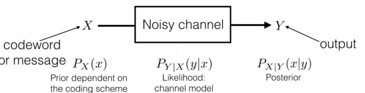
Inference refers to the process of drawings conclusions about some system or phenomenon in a rational way from observations related to it, and a possible a priori knowledge about it. We are here interested in statistical inference, that will be mainly applied to signal processing problems. Assume you have access to some data y, that have been generated through some process f related to some system properties of interest represented by the so-called signal s. The general relation linking these objects is given by:
y(θs,θf,θout) = Pout¡ f ¡s(θs)|θf¢ |θout¢ (3.1)
y is also referred as the observations, responses of the system or measurements in the present
thesis, s as the input, the predictors or signal in the present signal processing context. These two quantities can be a scalar, vectors, matrices, sets of labels, etc. f models the deterministic part of the data generating process and can be any function, whereas Pout is a stochastic
function linking the processed signal to the actual observations, used to model some kind of
noise. We will refer to it as the channel, this terminology coming from the communication
through it. In full generality, noise just means an incontrolable and undesired source of randomness that alters the observations of the system. In some cases, the noise can be correlated in some way to the signal s or process f such as in blind calibration [11], but in all the remaining, we will always consider the noise to be additive and uncorrelated with them. θs are parameters of the signal such as some of its statistical properties like mean,
variance, etc that can be known a priori or not.θf are those of the process f , for example the
number of Fourier coefficients taken in a partial discrete Fourier transform and finallyθout
are parameters of the channel, usually the statistical properties of the noise.
The problem is to estimate the signal s from the knowledge of the observations y, the process
f and the channel model Pout. The signal can be thought as a fixed realization of a random
process, for example a message some emitter has sent you or some image. The channelθout,
signalθsand processing functionθf parameters can be unknown too and it is a part of the task
to learn them as well. This can be done efficiently by statistical procedures such as expectation
maximization based methods that will be detailed in sec. 4.3.8.
For sake of readibility, we drop these parameters dependencies and re-write the general statistical inference model as:
y = Pout¡ f (s)¢ (3.2)
and the dependency on all the parameters of the problemθ := [θs,θf,θout] is now always
implicit.
An important remark is that in the present thesis, we mostly consider the signal s to be the unknown and f to be known as this interpretation is more relevant in the problems studied here. But actually, it would be perfectly equivalent to change their respective roles and let the process f becoming the unknown and s to be some known inputs. Depending on the problem it can be more natural to think of f as the unknow process that gave rise to the observations from controled inputs. It is really a matter of tastes. For example, in the classical reference [8],
f is most of the time the object of interest that we want to infer, but in [9], the authors adopted
the same convention as in the present thesis of always considering the signal s as the unknown. In examples where the unknown will be way more easily interpreted as f , it will be explicited, but in the rest s is always the infered quantity. Let us now define more precisely the different kind of statistical inference problems and give some vocabulary.
3.1.2 Inverse versus direct problems
The statistical inference problem (3.2) is by nature an inverse problem, in the sense that it consists in estimating properties of the system from some noisy observations about it, as opposed to the direct problem which is to obtain these observations. Getting observations about a complex system is usually quite easy compared to the associated inverse problem.
inverse problems. It is easy to gather data about the past stock prices which are observations correlated to many parameters of the market and to the behavior of plenty of buyers and sellers with their own strategies, but it is highly difficult to infer from these the future prices, that must be in some way correlated to previous ones. It is nowadays quite easy to measure time series of the activity of many neurons in parallel, but the inverse problem consisting in infering the network of connections between the neurons from which result these activities is very hard [12]. In an epidemic spreading of some disease, we can partially know at some time t who are contaminated or not and have some idea of the network of connections between people, from which we would like to infer back the source of the disease: the patient(s) zero [13]. The same question can be asked for the identifications of the source of an internet virus, where it is even more easy to get the network of connections between computers. These are highly non trivial inverse dynamical problems.
Statistical physics arised at the beginning of the 19t hto deal with direct problems. The aim was to link the microscopic properties of the system to its macroscopic ones, impossible to derive directly from the quantum mechanics, so the knowledge about the fundamental interactions between the atoms to the physical observables and order parameters like temperature, pres-sure, average magnetization, etc. But as we will see, the methodology of statistical physics and especially its tools to compute thermodynamical averages over some disorder is really useful in the signal processing and inverse problems context, where the atoms are replaced by the signal components, the interactions by the constraints extracted from the observations that must verify these variables and the order parameter or observable that we would like to predict is the typical error we will make in the inference of the signal. Fig. 3.1 is a table summarizing the connections between quantitities and notions of statistical physics and those of inference and signal processing (defined in this chapter).
3.1.3 Estimation versus prediction
Inference can be important for two main reasons. In one hand, one could aim at accurately estimating the signal that gave rise to the observations. If the signal models some system, inference really is about understanding it. For example in seismology, the signal s of interest could be the 3-d density field of the floor in some area. Perturbations by located explosions could be performed and the vertical displacement y of the floor in some places could be measured. The relation between the signal and the measures f , even non trivial is a priori obtainable (at least approximately) from the physics of waves propagations in complex media and the locations of the explosions. The noise here comes from the approximations in the modelisation of f and the partial measurements.
In another hand, one aim could be to perform predictions. In this setting, it is easier to think as the signal s to be known and it is the process f which becomes the unknown object of interest. The goal is to get an estimate of it ˆf which is able to accurately output responses to new, yet
Statistical physics Inference
Hamiltonian Cost function
Particules, atoms, spins Signal components
Microstates All the possible measured signals
Macrostate The final signal estimate ˆx, or estimator Physical phases: liquid, solid, gas, glass, etc Computational phases: Easy, hard,
impossible inference Boltzmann distribution Posterior distribution
Partition function Z (y, F,θ) Absolute probability of the measure P (y|θ,F)
External field Prior distribution
External parameters: temperature, volume, Noise variance∆, chemical potential, etc signal to noise ratio snr,
measurement rateα, signal densisty ρ, etc Order parameter: average magnetization, Mean square error M SE ,
correlation functions, Edwards-Anderson bit error rate, etc order parameter for spin glasses, etc
Quenched disorder: spin interactions, Observations, sensing or coding matrix impurities in the medium, etc and noise realizations
Free energy/entropy Potential function
Figure 3.1 – Relations between the statistical physics quantities and vocabulary with the inference and signal processing one, focused on the quantites useful in the present thesis, mainly related to compressed sensing and error correcting codes.
really interested in understanding the complex relations defining the market, so to estimate accurately f but more to be able to predict future prices y from the knowledge of previous ones s thanks to an estimator of the market process ˆf that have a good predictive potential,
despite it can have few common features with the true market behavior f , that can be way too complex to infer anyway from few partial observations.
All the problems that will be studied in depth in this thesis are estimation ones: we will always infer a signal that will be processed through some known transform f (s) = Fs, a matrix product.
3.1.4 Supervised versus unsupervised inference
All the previously discused examples and the model (3.2) belong to the class of supervised learning: problems where both observations y and the process f are known. It is thus a fitting problem and we can interpret the observations y associated with f as a training data set, that allows to "teach" the inference algorithm to perform its task in a supervised way. Again, the s and f roles can be switched without loss of generality. An example of a supervised problem is classification where one seeks for an algorithm able to class data in groups. For example if one want to design an algorithm able to distinguish between pictures of boys and girls, the