HAL Id: hal-00514212
https://hal-imt.archives-ouvertes.fr/hal-00514212
Submitted on 1 Sep 2010
HAL is a multi-disciplinary open access
archive for the deposit and dissemination of
sci-entific research documents, whether they are
pub-lished or not. The documents may come from
teaching and research institutions in France or
abroad, or from public or private research centers.
L’archive ouverte pluridisciplinaire HAL, est
destinée au dépôt et à la diffusion de documents
scientifiques de niveau recherche, publiés ou non,
émanant des établissements d’enseignement et de
recherche français ou étrangers, des laboratoires
publics ou privés.
An analytical model for evaluating outage and handover
probability of cellular wireless networks
Laurent Decreusefond, Philippe Martins, Thanh-Tung Vu
To cite this version:
Laurent Decreusefond, Philippe Martins, Thanh-Tung Vu. An analytical model for evaluating outage
and handover probability of cellular wireless networks. WPMC, Sep 2012, Taiwan. pp.1–5.
�hal-00514212�
An analytical model for evaluating outage and
handover probability of cellular wireless networks
L. Decreusefond, P. Martins, T. T. Vu
Institut Telecom Telecom Paristech
CNRS LTCI Paris, France
Abstract—We consider stochastic cellular networks where base
stations locations form a homogenous Poisson point process and each mobile is attached to the base station that provides the best mean signal power. The mobile is in outage if the SINR falls below some threshold. The handover decision has to be made if the mobile is in outage for some time slots. The outage probability and the handover probability is evaluated in taking into account the effect of path loss, shadowing, Rayleigh fast fading, frequency factor reuse and conventional beamforming. The main assumption is that the Rayleigh fast fading changes each time slot while other network components remain static during the period of study.
I. INTRODUCTION
In a wireless network, nodes can be modeled by fixed or stochastic pattern of points on the plane. Fixed points model can be finite or infinite and usually regular or lattice. This approach fails to capture the irregularity and randomness of a real network. For example, to model a wireless cellular network, the hexagonal cellular network is the model of this type most used. In reality, the base station (BS) nodes are usually fixed, it is not true that they are spastically periodical. Recently, stochastic model of nodes are more preferred. Node patterns can be represented by a stochastic process on the plane such as Poisson point process . It is worth to note that the stochastic models, although are more complicated at the first sight, usually lead to elegant and easy calculated formulas. In fact, all information obtained when studying both types of model are useful for the design or dimensioning processes of networks. In this paper we choose the stochastic approach and investigate a cellular network with homogeneous Poisson point process of BS.
However most of works relies on the assumption that a mobile once in the network is served by the nearest BS. This is due to considering path loss exponent model of radio propaga-tion and remove the effect of fading. This assumppropaga-tion results to a so called Poisson-Voronoi cells model (for example, [2], page 63). Most works consider only the effect of fading but only the slow fading such as log-normal shadowing or fast fading such as Rayleigh fading. Besides, most of works consider the well known exponent propagation model. In this paper, the proposed model is sightly more general. Firstly, we consider a general model of path loss. Secondly, we are interested in a system spastically static but some temporal evolutionary elements. More precisely, we include both random general
slow fading and Rayleigh fading but that the slow fading being static in time, and the Rayleigh fading changes each time slot. Thirdly, once considering this, we make a very natural assumption that the mobile is served by the BS that provides the most strong mean signal power in time (best server). The mean signal power depends on path loss and slow fading. This choice of serving BS can be made either by the mobile or the operator. Thus, it can be though that our model is a generalization of Poisson-Voronoi cell model. If we assume that each BS generates an independent copy of a continuous shadowing random such as the one in [12], one can interpret continuous cell form. However if each slow fading field generated by a BS is independent fading fields then the cells can not be analytically identified, in particular they can not be measurable. We do not address this issue in this paper. Nevertheless we make assumption that the slow fading value of BSs to a mobile is independent, so including all above cases.
Once the mobile is served by one BS, the signal received by this BS will be the useful signal, and we assume that the considered system other signal received by other BS using the same frequency is interference. It is not true if we consider for example an advanced system in which the base stations are cooperative. However our model covers almost all existing cellular networks. To model the frequency reuse, we add a independent mark on our Poisson point process of BSs. A BS interferes other BSs that have the same mark. In addition to the interferences, the local noise can intervene. In order to make communication with the BS, the signal-to-noise-plus-interferences ratio (SINR) at this mobile location must be excess some threshold, in this case the mobile is covered, in contrary it is in outage. If the mobile is in outage during a period of time, i.e for some consecutive time slots, a handover decision has to be made. It can be made by the mobile, the served BS, the network system or even by a neighbor BS. In this paper, we are interested in the calculation of the outage probability and the handover probability in explicit forms. Since we assumes a homogenous Poisson point process of BSs, but not fixed patterns, these results does not depend on the position of the mobile and can be considered as global, meaning on all MS on the network.
This present paper benefits from results in the literature. In [9], Haenggi shows that the path loss fading process is Poisson
2
point process in real line in the case of path loss exponent model. In [1], [2] and [3], Baccelli and al. find analytical expressions for outage probability of networks where each node tries to connect with a destination of fixe distance or the nearest node in case of Rayleigh fading. In [6], Kelif and al. find a outage probability expression for cellular network by mean of the so-called fluid model. In [5], Ganti and al. find the interesting results about temporal and spatial correlation of wireless networks. In [10] and [11], outage probability of regular hexagonal cellular networks with reuse factor and adaptive beamforming is studied by simulation.
This paper is organized as following. In the section II we describe our model. In this section III we show that the path loss shadowing is a Poisson point process in real line. In the section IV we calculate outage probability. In the section V we calculate the handover probability. Section VI shows the numerical results and the difference between our model and the traditional hexagonal model.
II. SYSTEM MODEL AND SCENARIO
A. Propagation model
The signal radio propagation modelling is complicated, usually divided by a deterministic large scale path loss and the random fading components. The large scale path loss describes the channel at a microscopic level. If there are a BS (base station) located at y and an mobile located at x and the transmission powerP , the mobile’s received signal has the average power L(y− x)P where L is the path loss function. We assume that L is measurable function on R2.
The most used path loss function is the path loss exponent law L(z) = K|z|−γ where |z| refers to the Euclid norm of
z. The parameter K depends on the frequency, the antenna height,... while the path loss exponent γ characterizes the environment under study.γ is typically in the range of (2, 4), it may be greater if the environment is very dense urban. In fact, this path loss model is not correct for small distances and has infinite mean of interference for Poisson patterns of BSs [1]. To avoid theses problems, one can use the modified path loss exponent model L(z) = K(max{R0,|z|})−γ whereR0
is a reference distance.
In addition to the deterministic large scale effect, there are two random factors can be considered. The first, called
shadowing or shadow fading, represents the signal attenuation
caused by a large obstacle such as building. The second, called
fast fading, represents the impact of multipath phenomena, or
in other word many objects scatter the signal. The shadowing can be considered as constant during a period of communi-cation of the mobile while the fast fading changes each time slot. If there is no beamforming technique is used, the received signal power from BSy to MS x at the time slot l will be
Pyx[l] = ry,x[l]hyxL(y− x)P, (1)
where{hyx}x,y∈R2 are copies of a random variableH while
{ryx[l]} are independent copies of R which is an exponential
random variable of mean 1/µ. We suppose that for each x, the random variableshyx for ally∈ R2are independent. We
definepH the probability density function ofH and FH(β) =
P (H≥ β) =R∞
β pH(t)dt. The most used shadowing random
model is log-normal shadowing, for whichH is a log-normal random variable. In this case, we can writeH∼ 10G/10where
G∼ N (0, σ2).
In short word, we suppose that during the period of study, the shadowing remains constant while the Rayleigh fast fading changes at each time slot.
Consider the path loss shadowing process Ξ = {ξi =
(hyxL(y− x)P )−1}. We make the following assumptions:
Assumption 1: For each x∈ R2,
{hyx}y∈R2 are
indepen-dent.
Assumption 2: H admits a continuous probability density
function on(0,∞).
Assumption 3: Define B(β) = R
R2FH((L(z)P β)−1)dz,
then0 < B(β) <∞ for all β > 0.
By the displacement theorem we will show thatΞ is a sim-ple Poisson point process in the real line(0, +∞) (proposition 1) of intensityΛ(dt) = λBB′(β) > 0. Hence we have the right
to reorderΞ such that ξ0< ξ1< ... and for simplicity we do
it.
B. Poisson point process of BSs
We assume the homogenous Poisson point process of BSs ΠB = {y0, y1, ...} of intensity λB on R2, each BS transmit
has constant transmitted powerP . For any details on Poisson point process we refer to [2].
Assumption 4: Once being in the network the mobilex is
firstly attached to (or served by) the BSs that provide the best
average signal strength in time. In other word, it is attached
byy0(after reordering and renumberingΞ).
C. Beamforming model
We consider the conventional beamformer technique with nt antennas. The power radiation pattern for a conventional
beamformer is a product of array factor and radiation pattern of a single antenna. Ifφ is the look direction (toward which the beam is steered), the array gain in the directionθ is given by ( [11], [10]):
sin2(ntπ2(sin(θ)− sin(φ))
ntsin2(π2(sin(θ)− sin(φ))
g(θ),
where g(θ) is the gain in the direction θ with one antenna. For simplicity we assume that the BS always steers to the direction of the serving MS and the gain g(θ) is positive constant on(−π/2, π/2) and 0 otherwise (zero front-to-back power ratio). Hence, the interference signal power from a BS to a MS attached by an other BS using the same frequency in the directionθ will be reduced by a factor of:
a(θ) = 1{θ∈(−π/2,π/2)}sin 2(n tπ2(sin(θ))) n2 tsin2(π2(sin(θ))) ·
If the beamforming technique is not used, we will simply use a(θ) = 1.
D. Frequency reuse
We add a mark to each BSsei. The markseiare independent
copies of the random variableE who is uniformly distributed on {1, 2, ..., k} where k will be called the frequency reuse factor. The BSs that have the same mark interfere between themselves. Our reuse model can be considered as the worst case where the bandwidth is divided into k subband and each BS is randomly attributed a sub band. It is contrast to the hexagonal network pattern where the interfering BS must be placed far from a reference BS.
E. SINR
Assume that each other BS using the same frequency is always serving a MS, and the MS x is in the direction θi
which is i.i.d chosen on(−π, π) of the BS i. The SINR at the time slot l is defined as:
sx[l] = ry0x[l]ξ −1 0 N +P i6=01{ei=e0}a(θi)ryix[l]ξ −1 i , (2)
where N is a constant noise power. The term Ix =
P
i6=b(x)1{ei=e0}a(θi)ryix[l]ξi−1 is the sum of all
interfer-ences. In order to make communication with the attached BS, the SINR must not fall below some threshold T .
F. Handover decision
We consider a simple SINR based decision. The handover should be made if the MS is in outage forn consecutive time slots.
G. Scenario
The scenario is as following:
• Realization of a snapshot of BSsyi, slow fadinghyixand
the frequency ei.
• Attachment of mobilex to best BS, (y0 after reordering
Ξ).
• Realization of the directionsθi for interfering BS yi. • At time slot l, realization of Rayleigh fast fading ryix[l]
and calculate the SINRsx[l]. If sx[l] < T then the mobile
is in outage otherwise it is covered.
• If the mobile is in outage for n consecutive time slots then the handover should be made.
The outage probability is then po(T ) = P (sx[l] < T ) and
the handover decision probability is pho(T ) = P (sx[l] <
T, ..., sx[l + n− 1] < T ). We also define the coverage
probabilitypC(T ) = P (sx[l]≥ T ).
H. Interference limited case
We are particularly interested in the interference limited regime when the noise powerN is negligible or nearly equal to zero as it happens usually in a real network. We can set N = 0. The outage probability calculated in the interference regime can be considered as an upper bound for the outage probability in the general case.
III. POISSON POINT PROCESS OF PATH LOSS SHADOWING
A. General case
Proposition 1: Ξ is a Poisson point process on R+ =
(0,∞) with intensity density Λ(dt) = λBB′(t)dt.
Proof: Define the marked point process Πx =
{yi, hyix}∞i=0. It is a Poisson point process of intensity
λBdy ⊗ fH(t)dt because the marks are i.i.d. We consider
the probability kernel p((z, t), A) = 1{(L(z)P t)−1∈A} for all
Borel A ∈ R+ and apply the displacement theorem ( [2],
theorem 1.3.9) to obtain that the point process Ξ is Poisson point process of intensity
Λ(A) = λB
Z
R2⊗R
1({L(z)tP )−1∈A}pH(t)dzdt·
We now show thatΛ([0, β]) = λBB(β). Indeed,
Λ([0, β]) = λB Z R2⊗R 1{t≥(βP.L(z)P )−1}pH(t)dzdt = λB Z R2 FH((βL(z)P )−1)dz = λBB(β)·
Finally B(β) admits a derivative: B′(β) = β−2 Z R2 1 L(z)PpH((βL(z)P ) −1)dz· (3)
This concludes the proof.
The CDF and PDF of ξm are easily derived according to
the property of Poisson point process:
Lemma 1: The complementary cumulative distribution
function ofξm is given by:
P (ξm> t) = e−λBB(t) m X i=0 (λBB(t))i i! , (4)
and its probability density function is given by pξm(t) = λ
m+1
B B′(t)B(t)
me−λBB(t)· (5)
Proof: The event ”ξm> t” is equivalent to the event ”in
the interval [0, t] there is at most m points” and the number of points in this interval follows a Poisson random variable of mean λBB(t), so: P (ξm< t) = e−λBB(t) m X i=0 (λBB(t))i
The PDF is thus given bypξm(t) =−
d
dtP (ξm< t), and after
some simple manipulations we obtain the equation (5)
B. Special cases
In this section we derive closed forms for B(β) in some special cases.
4
a) Path loss exponent model:
Lemma 2: If L(z) = K|z|−γ then: B(β) = C.β2γ, (6) whereC = π(P K)2γE(H 2 γ). Proof: We have: B(β) = 2π Z ∞ 0 r1{tP Kβ≥rγ}pH(t)drdt = 2π Z ∞ 0 pH(t)dt Z (tKP β)1/γ 0 rdr = π(P K)γ2β 2 γ Z ∞ 0 pH(t)t 2 γdt = π(P K)γ2E(H2γ)βγ2·
Hence the result.
Remark that this result can be derived from [9]. We observe that the distribution of the point process Ξ does depend only onE(H2γ) but not on the distribution of shadowing H itself.
This phenomenon can be explained as in [4](page 159).
b) Modified path loss exponent model:
Lemma 3: If L(z) = K(max{R0,|z|})−γ then:
B(β) = C1β 2 γ Z ∞ Rγ0 βP K t2γp H(t)dt, (7) whereC1= π(P K) 2 γ. In addition, we have: B′(β) = 2 γβ −1B(β) + πR2 0pH( R γ 0 P Kβ)· (8) If the slow fading is lognormal shadowingH∼ 10G/10where
G∼ N (0, σ2) we have: B(β) = C1β 2 γe(2σ1γ ) 2 Q(− ln β − ln(P KR −γ 0 ) σ1 − 2σ1 γ ) (9) whereQ(u) =√1 2π R∞ u e−u 2
/2du is the Q-function and σ 1= σ ln 10
10 .
Proof: Similarly to the pathloss exponent model case, we
have: B(β) = 2π Z R2 rFH((max{R0, r})−γ(P Kβ)−1)dr = πR02FH(Rγ0(P Kβ)−1) + +2π Z ∞ Rγ 0 βP K pH(t)dt Z (tKP β)1/γ R0 rdr = C1β 2 γ Z ∞ Rγ0 P Kβ tγ2p H(t)dt·
We obtain the equation (7). Derivative two sides of that equation and do some simple manipulations we obtain the
equation (8). In the case of lognormal shadowing we have: B(β) = C1β 2 γ Z ∞ Rγ 0 P Kβ 1 p2πσ2 1t t2γe− (ln t)2 2σ2 1 dt = C1β 2 γ Z ∞ ln R γ 0 P Kβ 1 p2πσ2 1 e2uγ e− u2 2σ2 1du = C1β 2 γe(2σ1γ ) 2Z ∞ ln R γ 0 P Kβ 1 p2πσ2 1 e− (u−2σ21 γ )2 2σ2 1 du·
Here the results.
As a consequence, both the exponent path loss model and its modified model satisfy the assumption 3.
IV. OUTAGE ANALYSIS
A. General case
Here, we remark that the outage probability and the cover-age probability do not depend on the time index. So we can drop the time slot parameter in this section. The expression of the SINR can be rewritten as:
sx= ry0xξ −1 0 N +P i6=01{ei=e0}a(θi)ryixξi−1 · (10)
The outage probability is calculated as below:
Theorem 1: The outage probability is given by
po= 1− λB Z ∞ 0 B′(β)e−λBB(β)−NT µβ−2πkλBD(β)dβ whereD(β) =Rπ −πdθ R∞ β B′(ξ) dξ 1+ξ(T βa(θ))−1.
Proof: To calculate the outage probability P (sx < T ),
we will calculate the coverage probabilityP (sx≥ T ).
We first consider the conditional probabilityP (sx≥ T |ξ0=
β). Because ry0x is an exponential random variable of mean
1/µ we have: P (sx≥ T |ξ0= β) = P (ry0x≥ T β(N + Ix(β))|ξ0= β) = E(e−µT β(N+Ix(β)) |ξ0= β) = e−NT µβL Ix(β)(T µβ)
whereIx(β) is the distribution of the random variable Ixgiven
on the event (ξ0 = β)) andLIx(β) is its Laplace transform.
Conditioning on the event(ξ0= β) the point process{ξi}i>0
is a Poisson point process on(β,∞) with intensity λBB′(ξ)dξ
according to the strong Markov property. By thinning theorem, the point process {ξi}{i>0,ei=e0} is a Poisson point process
on (0, β) with intensity λB
k B′(ξ)dξ. Hence, LIx(β) can be
calculated as follows ( [2], shot noise theory): LIx(β)(u) = e −Rβ∞2πkλBB′(ξ)(1−E(e−a(θ)uξ− 1 R))dξ = e−2πkλB R∞ β B ′(ξ)dξR∞ 0 dr Rπ −πµe −µr(1−e−a(θ)urξ−1)dθ = e−2πkλB Rπ −π dθR∞ β B ′(ξ) dξ 1+ξµ(ua(θ))−1· We get that: P (sx≥ T |ξ0= β) = = e−NT µβ−2πkλB Rπ −πdθ R∞ β B ′(ξ) dξ 1+ξ(T β.a(θ))−1,
thus
= e−NT µβ−2πkλBD(β)· (11)
Since the distribution density of ξ0 is λBB′(β)e−λBB(β)
(proposition 1), by averaging over allξ0we obtain the equation
(11).
B. Special cases
c) Interference limited:
Collary 1: In the interference-limited regime, we have
po(T ) = 1− λB
Z ∞
0
B′(β)e−λBB(β)−2πkλBD(β)dβ· (12)
d) Path loss exponent model:
Collary 2: IfL(z) = K|z|−γ we have: po(T ) = 1− Z ∞ 0 e−Mα−Gα γ 2 dα (13) whereM := M (k, T, γ) = 1+2πk1 Rπ −πdθ R∞ 1 du 1+(T.a(θ))−1uγ2 andG = N T µ(λBC)− γ 2.
Proof: Since B(ξ) = C.ξγ2 and B′(ξ) = 2C
γ ξ 2 γ−1 we have: D(β) = Z π −π dξ Z ∞ β 2C γ ξ 2 γ−1 dθ 1 + ξ(T βa(θ))−1 = C.β2γ Z π −π dθ Z ∞ β d(βξ)2γ 1 + ξβ(T a(θ))−1 = C.β2γ Z π −π dθ Z ∞ 1 du 1 + (T a(θ))−1uγ2·
Plug it into (11) we have: pc(T ) = Z ∞ 0 2λBC γ β 2 γ−1e−λBCMβ 2 γ−NT µβ dβ = Z ∞ 0 e−Mα−Gα γ 2 dα·
Remark that if γ = 4, we can find that:
M = 1 + 1 2πk Z π −π dθ Z ∞ 1 du 1 + (T a(θ))−1u2 = 1 + 1 2πk Z π −π pT a(θ)(π 2 − arctan 1 pT a(θ))dθ and po(T ) = 1− e M 2 4G Z ∞ 0 e−( √ Gα+ M 2√G) 2 dα = 1− √ 2π G e M 2 4GQ( M 2√G)·
e) Interference limited and path loss exponent model:
In this case, the outage probability is easily derived from (13) by setting N = 0.
Collary 3: IfL(z) = K|z|−γ andN = 0 we have:
po(T ) = 1− 1
M· (14)
C. Observations and interpretations
Some interesting facts are observed from above results:
• Rewrite the expression of SINR as
sx[l] = ry0x[l]ξ −1 0
µN +P
i6=01{ei=e0}a(θi)ryix[l]ξi−1
where ry0x[l] = µryix[l]. Since ryx[l] is an exponential
random variable of mean 1/µ, ry0x[l] is an exponential
random variable of mean1. Hence by the above equation it is expected that the outage probability depends on the productµN but not directly on µ and N . It is increasing function of N µwhich is confirmed by the equation (11). The fact that the outage probability is the increasing function ofµ and N is quite natural, the increase of noise or the degrade of the channel fast fading always makes the system work worsts.
• It is also expected that in the interference limited case
(N = 0) the outage probability does not depend on µ. It is confirmed by the equation (12). Physically it means that in the absence of noise, the fast fading increases or degrades the channels to the MS of the serving BS and the interfering BS at the same level, thus the SINR will not change.
• In the interference limited and exponent path loss model case, the outage probability does not depend on µ, the BS density λB, or the distribution of shadowing H.
It is due to the scaling property of the exponent path loss and the homogeneous Poisson point process. The outage probability is a decreasing function of the path loss exponentγ, reflecting the fact that bad propagation environment degrades the received SINR.
• In the presence of noise N > 0 and exponent path loss model case, the outage probability is a increasing function ofλB. Hence, it can be thought that the more an operator
installs BSs, the better the network is. In addition, if the density of BSs goes to infinite then outage will never occur. However it is not true. In fact, if the density of BSs is very high, the distance between a MS and its serving BS and some interfering BSs is relatively close. Here, the exponent path loss model is no longer valid since it is not accurate at small distance. If the modified exponent path loss is used which is more appreciate, the outage probability must converge to 0. The outage probability is also a increasing function ofE(Hγ2), and
if the shadowingH follows lognormal distribution then the outage probability will be increasing function of σ. We recover an other well known fact: the increase of uncertainty of the radio channel degrades the performance of the network.
V. HANDOVER ANALYSIS
A. General case
If the MS is in outage in n consecutive time slots, a handover decision has to be made. Keep in mind that only the Rayleigh fast fading changes each time slot, and the other
6
network components do not change. LetAl be the event that
the mobile being in outage in the time slotl, and Ac
l its
com-plement and observe that in fact P (∩m
i=1Acji) = P (∩
m i=1Aci).
By definitionpho:= P (∩ni=1Al+i−1) = P (∩ni=1Ai). We have
pho = 1 + n X m=1 (−1)m X j16=...6=jm∈{1,..,n} P (∩m i=1Acji) = 1 + n X m=1 (−1)m n! m!(n− m)!P (∩ m i=1Aci)·
Theorem 2: The handover probability is given by:
pho= 1 + n X m=1 (−1)m n! m!(n− m)!qm, whereqm= P (∩mi=1Aci) is given by:
qm= Z ∞ 0 λBB′(β)e−λBB(β)−NT µβ− λB 2πkDm(β)dβ, andDm(β) =R π −πdθ R∞ β B′(ξ)(1− ( 1 1+T βa(θ)ξ−1) m)dξ. Proof:
We need to calculate the probabilityP (∩m
i=1Aci) that is the
probability that the mobile is covered inm different time slots. The calculation is similar the that in section IV. We begin with calculating the conditional probabilityP (∩m
i=1Aci|ξ0= β): P (∩m i=1Aci|ξ0= β) = P (sx[1]≥ T, ..., sx[m]≥ T |ξ0= β) = P (ry0x[i]≥ β(T N + Ix[i])i = 1..m|ξ0= β) = E(e−µ(mT Nβ+P m i=1Ix(β)[i])|ξ0= β) = e−mNT µβLPm i=1Ix(β)[i] (T µβ) whereIx(β)[i] is the distribution of the random variable Ix[i]
given(ξ0= β). We have : m X i=1 Ix(β)[i] = ∞ X j=1 1{ei=e0}ξ −1 i a(θi)( m X i=1 ryix[i])·
As the random variables ryix[i] are independent copies of
the exponential random variable R, the random variables Pm
i=1ryix[i] are also i.i.d and the common Laplace transform
of the later are : LPm
i=1ryix[i]
(u) = (LR(u))m
= ( µ
µ + u)
m
· The Laplace transform ofPm
i=1Ix(β)[i] is now:
LPm i=1Ix(β)[i] (u) = e−2πkλB Rπ −πdθ R∞ β B ′(ξ)(1−( µ µ+a(θ)ξ−1 u) m)dξ · The conditional probability is then given by:
P (∩m
i=1Aci|ξ0= β) = e−mNT µβ−
λB 2πkDm(x)
· By averaging with respect to ξ0, we have:
qm= Z ∞ 0 λBB′(β)e−λBB(β)−NT µβ− λB 2πkDm(β)dβ · This concludes the proof.
B. Special cases
We can obtain more closed expression for qm in some
special cases.
f) Interference limited:
Collary 4: In the interference limited regime N = 0, we
have: qm= Z ∞ 0 λBB′(β)e−λBB(β)− λB 2πkDm(β)dβ·
g) Path loss exponent model:
Collary 5: IfL(z) = K|z|−γ then: qm= Z ∞ 0 e−Mmα−Gα γ 2 dα whereMm= 1 +2πk1 R−ππ dθR1∞(1− ( 1 1+T a(θ)u−γ2) m)du.
Proof: The proof follows the same lines as the proof of
2
Closed expression ofqm is obtained in the caseγ = 4:
qm= √ 2π G e M 2m 4G Q(Mm 2√G)·
h) Interference limited and path loss exponent model:
Collary 6: IfN = 0 and L(z) = K|z|−γ we have:
qm=
1 Mm·
C. Observations and interpretations
Some interesting facts are observed from above results and they are similar to the properties of outage probability:
• The handover probability is increasing function ofN µ.
• In the interference limited and exponent path loss model case, the handover probability does not depend onµ, the BSs density λB, nor the distribution of shadowing H.
The handover probability is a decreasing function of the path loss exponentγ.
• In the presence of noise N > 0 and exponent path
loss model case, the handover probability is a increasing function of λB. Thus, in this case the more an operator
installs BSs, the less a MS has to do handover. But it is not true in a real system. As previously explained, in the case of very dense BSs, the pathloss exponent model is no longer accurate for small distance. The handover probability is also a increasing function of E(Hγ2),
therefore if the shadowing H is lognormal shadowing the handover probability will be increasing function of σ.
VI. NUMERICAL RESULTS AND COMPARISON TO THE HEXAGONAL MODEL
We place a MS at the origin o and consider a region B(o, Rg) where Rg= 10.000(m). The BSs are distributed as
a Poisson point process in this region. The path loss exponent model is considered. The default values of model are placed on the table I. They are not changed throughout the simulation.
TABLE I
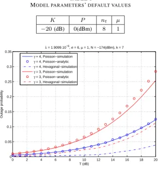
MODEL PARAMETERS’DEFAULT VALUES
K P nt µ −20(dB) 0(dBm) 8 1 0 2 4 6 8 10 12 14 16 18 20 0 0.05 0.1 0.15 0.2 0.25 0.3 0.35 T (dB) Outage probability λ = 1.9099.10−6, σ = 6, µ = 1, N = −174(dBm), k = 7 γ = 4, Poisson−simulation γ = 4, Poisson−analytic γ = 4, Hexagonal−simulation γ = 3, Poisson−simulation γ = 3, Poisson−analytic γ = 3, Hexagonal−simulation
Fig. 1. Outage probability vs SINR threshold
In literature, the hexagonal model is widely used and studied so we would like to compare two models. For a fair compar-ison, the density of BSs must be chosen to be the same, i.e the area of a hexagonal cell will be1/λB. Unlike the Poisson
model where each BS is randomly assigned a frequency, in the hexagonal model, the frequencies are well assigned so that an interfering BS is far from the transmitting BS and BSs of different frequency are grouped in reuse patterns. The reuse factor k in the hexagonal model is determined by k = i2+ j2+ ij where integers i, j are the relative location of
co-channel cell. The MS is uniformly chosen on the surface of the center cell. The same signal propagation model and the scenario described in the section II-G are applied in the hexagonal model.
The figure 1 shows the outage probability versus the SINR threshold of the Poisson model and the hexagonal model in the case k = 7. As we can see, the outage probability in the case of Poisson model is always greater than that of hexagonal model which is intuitive. The different is about 8 (dB) in the caseγ = 4 and 6(dB) in the case γ = 3.
In the figure 3 plotted the outage probability as a function of γ. We can see that the outage probability is a decreasing function ofγ as theoretically observed. In the figure 4 plotted the handover probability versus the SINR threshold of Poisson model and hexagonal model. If the reuse factork increase, the MS has to do less handover. Thus, increase the reuse factor has a positive effect on the system performance not only in term of outage but also in term of handover.
VII. CONCLUSION
In this paper we have investigated the outage and handover probabilities of wireless cellular networks taking into account the reuse factor, the beamforming, the path loss, the slow
0 2 4 6 8 10 12 14 16 18 20 0 0.01 0.02 0.03 0.04 0.05 0.06 0.07 0.08 0.09 0.1 T (dB) Handover probability N = −174 (dBm), k = 7, σ = 6 (dB), µ = 1 Hexagonal model, γ = 3, n = 6 Hexagonal model, γ = 3, n = 3 Poisson model, γ = 3, n = 3 Poisson model, γ = 3, n = 6 Hexagonal model, γ = 4, n = 6 Hexagonal model, γ = 4, n = 3 Poisson model, γ = 4, n = 3 Poisson model, γ = 4, n = 6
Fig. 2. Handover probability vs SINR threshold
2.4 2.6 2.8 3 3.2 3.4 3.6 3.8 4 0 0.01 0.02 0.03 0.04 0.05 0.06 0.07 0.08 0.09 0.1 γ Outage probability N = −174 (dBm), T = 5 (dB), σ = 6(dB), µ = 1 k = 7 k = 3 k = 12
Fig. 3. Outage probability vs path loss exponent γ, Poisson model
2.4 2.6 2.8 3 3.2 3.4 3.6 3.8 4 0 0.005 0.01 0.015 0.02 0.025 γ Handover probability N = −174 (dBm), T = 5 (dB), σ = 6(dB), µ = 1 k = 3 k = 7 k = 12
Fig. 4. Handover probability vs path loss exponent γ, Poisson model, n = 3
fading and the fast fading. We valid our model by simulation and compare numerical results to that of hexagonal model. The analytical expressions derived in the this paper can be considered as an upper bound for a real system.
8
REFERENCES
[1] F. Baccelli, B. Blaszczyszyn and P. Muhlethaler , An Aloha protocol for multihop mobile wireless networks. IEEE Trans. Inf. Theory 52, 421-436, 2006
[2] F. Baccelli and B. Blaszczyszyn , Stochastic Geometry and Wireless Networks, Volume I - Theory vol. 3, No 3-4 of Foundations and Trends in Networking, NoW Publishers, 2009
[3] F. Baccelli and B. Blaszczyszyn , Stochastic Geometry and Wireless Networks, Volume II - Applications vol. 4, No 1-2 of Foundations and Trends in Networking, NoW Publishers, 2009
[4] M. Haenggi and R. Krishna Ganti, Interference in Large Wireless Net-works, Vol. 3, No. 2 of Foundations and Trends in Networking, NoW Publishers, 2009
[5] R. K. Ganti and M. Haenggi, Spatial and Temporal Correlation of the Interference in ALOHA Ad Hoc Networks, IEEE Communications Letters, vol. 13, pp. 631-633, Sept. 2009
[6] J. M. Kelif, M. Coupechoux and Ph. Godlewski, Spatial Outage Proba-bility for Cellular Networks, IEEE Globecom, 2007
[7] V.I. Mordachev, S. Loyka, On Node Density Outage Probability Tradeoff in Wireless Networks, IEEE Journal on Selected Areas in Communica-tions (Special Issue on Stochastic Geometry and Random Graphs for the Analysis and Design of Wireless Networks), v. 27, N. 7, pp. 1120-1131, Sep. 2009
[8] M. Haenggi, J. G. Andrews, F. Baccelli, O. Dousse, and M. Franceschetti, Stochastic Geometry and Random Graphs for the Analysis and Design of Wireless Networks, IEEE Journal on Selected Areas in Communications, vol. 27, pp. 1029-1046, Sept. 2009. Invited Paper
[9] M. Haenggi, A Geometric Interpretation of Fading in Wireless Networks: Theory and Applications, IEEE Trans. on Information Theory, vol. 54, pp. 5500-5510, Dec. 2008
[10] X. Lagrange, CIR cumulative distribution in a regular network, internal research report, ENST Paris, 2000
[11] M. Maqbool, M. Coupechoux and Ph. Godlewski, Comparison of Various Frequency Reuse Patterns for WiMAX Networks with Adaptive Beamforming, IEEE VTC Spring, 2008
[12] D. Catrein and R. Mathar, Gaussian random fields as a model for spatially correlated log-normal fading, IEEE ATNAC, 2008