Influence of the nonlocal effects on the near-field radiative heat transfer

(1)

THÈSE

Pour l'obtention du grade de

DOCTEUR DE L'UNIVERSITÉ DE POITIERS École nationale supérieure d'ingénieurs (Poitiers) Institut de chimie des milieux et matériaux de Poitiers - IC2MP

(Diplôme National - Arrêté du 7 août 2006)

École doctorale : Sciences et ingénierie en matériaux, mécanique, énergétique et aéronautique -SIMMEA (Poitiers)

Secteur de recherche : Energétique, thermique, combustion

Présentée par :

Farah Singer

Influence of the nonlocal effects on the near-field radiative heat transfer

Directeur(s) de Thèse : Karl Joulain, Younès Ezzahri

Soutenue le 19 décembre 2014 devant le jury Jury :

Président Sebastian Volz Directeur de recherches CNRS, EM2C, Paris

Rapporteur Philippe Ben Abdallah Directeur de recherches CNRS, Institut d'Optique, Paris Rapporteur Rodolphe Vaillon Directeur de recherches CNRS, CETHIL, INSA, Lyon Membre Karl Joulain Professeur, Pprime, ENSIP, Université de Poitiers Membre Younès Ezzahri Maître de conférences, Pprime, Université de Poitiers Membre Pierre-Olivier Chapuis Chargé de recherches CNRS, CETHIL, INSA, Lyon

Pour citer cette thèse :

Farah Singer. Influence of the nonlocal effects on the near-field radiative heat transfer [En ligne]. Thèse Energétique, thermique, combustion. Poitiers : Université de Poitiers, 2014. Disponible sur Internet <http://theses.univ-poitiers.fr>

(2)

Thesis

For obtaining the grade of

DOCTOR OF THE UNIVERSITY OF POITIERS

Ecole Nationale Supérieure d’Ingénieurs de Poitiers

Ecole Doctorale : Ecole Doctorale Sciences et Ingénierie en Matériaux, Mécanique, Energétique et Aéronautique

Presented by

Farah SINGER

INFLUENCE OF THE NONLOCAL EFFECTS ON THE NEAR-FIELD

RADIATIVE HEAT TRANSFER

Director and supervisor of the thesis: Pr. Karl JOULAIN

Co-supervisor of the thesis: Dr. Younès EZZAHRI

Defended on 19 december 2014 infront of the Commission of examination

JURY

Philippe BEN-ABDALLAH Senior Researcher at CNRS, Institut d’Optique, Paris Reviewer Rodolphe VAILLON Senior Researcher at CNRS, CETHIL, Lyon Reviewer Sebastian VOLZ Senior Researcher at CNRS, EM2C, Paris Examinar Pierre-Olivier CHAPUIS Researcher at CNRS, CETHIL, Lyon Examinar Younès EZZAHRI Associate Professor at University of Poitiers, PPRIME Institute Examinar Karl JOULAIN Professor at University of Poitiers, PPRIME Institute Examinar

(3)

Table of figures

Figure 1.1: The electromagnetic spectrum……….………..…..4

Figure 1.2: The spectral emissive blackbody power as given by Planck’s law………....6

Figure 1.3: A schematic diagram of the Evanescent waves………..…………....8

Figure 1.4: A schematic diagram of the geometry of the (1-interface) system………12

Figure 1.5: Two parallel semi-infinite material planes separated by a vacuum gap of width d……….………13

Figure 1.6: Variation of the RHTC between two semi-infinite 6H- SiC parallel planes for the local model case………..…………...19

Figure 1.7: Behaviors of the spectral energy flux and the spectral EM energy density………...22

Figure 1.8: Dispersion relation for surface phonon-polaritons at a SiC-Vacuum interface…….24

Figure 2.1: Variation of the RHTC between two semi-infinite Al parallel planes, for the local model case……….…...34

Figure 2.2: Variation of the RHTC between two semi-infinite Al parallel planes, for the Lindhard-Mermin nonlocal model case………...…...38

Figure 2.3: Variation of the RHTC between two semi-infinite Al parallel planes, for the local and the nonlocal model cases………...39

Figure 2.4: Plot of the transmission coefficient , for the local case (a) and the nonlocal case of Lindhard-Mermin model (b)………..…40

Figure 3.1: The dispersion relation of surface optical phonons of semi-infinite ionic crystals as given by Kliewer and Fuchs……….……...45

Figure 3.2: Variation of the RHTC between two semi-infinite 6H- SiC parallel planes, for the first suggested nonlocal model case………...49

Figure 3.3: Variation of the total RHTC between two semi-infinite 6H- SiC parallel planes, for the local and the first suggested nonlocal model cases………..50

Figure 3.4: Variation of 𝐼𝑚(𝑟_3𝑚𝑃 ) for the local case (a) and the 1st suggested nonlocal case (b)………..……….51

Figure 3.5: Plot of the transmission coefficient, for the local case (a) and the 1st suggested nonlocal case (b)………...52

Figure 3.6: Variation of the transmission coefficient for 𝜔 = 𝜔𝑇𝑂, for the first suggested nonlocal case……….……...53

(7)

Figure 3.7: Variation of the RHTC between two semi-infinite 6H- SiC parallel planes, for the 2nd suggested nonlocal model case………..…...…56 Figure 3.8: Variation of the total RHTC between two semi-infinite 6H- SiC parallel planes, for the local and the 2nd suggested nonlocal model cases………...…...57 Figure 3.9: Variation of 𝐼𝑚(𝑟_3𝑚𝑃 ) for the local case (a) and the 2nd suggested nonlocal case (b)……….…...59 Figure 3.10: Plot of the transmission coefficient, for the local case (a) and the 2nd suggested nonlocal case (b)………..…..…60 Figure 3.11: Variation of the transmission coefficient for 𝜔 = 𝜔_𝑇𝑂, for the 2nd suggested nonlocal model………...…....61 Figure 3.12: Plot of the transmission factor for the 2nd suggested nonlocal model by considering

d=0 and 𝐾 = 𝑛𝑞_𝐵………..…61

Figure 3.13: Variation of the RHTC between two semi-infinite 6H- SiC parallel planes, for the third suggested nonlocal model case when_{𝑙 = 𝑟}₀………...…65 Figure 3.14: Variation of the total RHTC between two semi-infinite 6H- SiC parallel planes, for the local case and the 3rd suggested nonlocal model case when 𝑙 = 𝑟0……….65 Figure 3.15: Variation of the total RHTC between two semi-infinite 6H- SiC parallel planes, for the local case and the 3rd suggested nonlocal model case when_{𝑙 = (1,2, … 10)𝑟}₀.…………....66 Figure 3.16: Plot of the function for the local case (l=0) and the 3rd suggested nonlocal cases (𝑙 = 1𝑟0, 3𝑟0, 6𝑟0, 8𝑟0 𝑎𝑛𝑑 10𝑟0)……….……...69 Figure 3.17: Variation of the saturation value of the RHTC between two semi-infinite parallel 6H-SiC planes, as function of the coherence parameter l………..70 Figure 3.18: Variation of ℎ_𝑟𝑎𝑑𝑒𝑣𝑎𝑛 𝑝(𝑇, 𝑙) as function of the average temperature T for the cases

when _{𝑙 = 1𝑟}_{0, 5𝑟}_{0 𝑎𝑛𝑑 10𝑟}₀……….…..…...72

Figure 4.1: A schematic diagram showing the incidence of an EM wave on the interface separating the local medium (vacuum) from the local dielectric medium (a), and the nonlocal dielectric medium (b)………..…..…...78 Figure 4.2: A schematic diagram showing that an excitation at a point r’ produces a response at

a point r………..…....81

Figure 4.3: Variation of the RHTC between two semi-infinite 6H-SiC parallel planes, for

Rimbey and Mahan nonlocal model……….…....87

Figure 4.4: Variation of the RHTC, between two semi-infinite 6H-SiC parallel planes, for Agarwal et al. nonlocal model………..……...87

(8)

Figure 4.5: Variation of the RHTC between two semi-infinite 6H-SiC parallel planes, for Ting

et al. nonlocal model………..………88

Figure 4.6: Variation of the RHTC between two semi-infinite 6H-SiC parallel planes, for Kliewer and Fuchs nonlocal model………...88 Figure 4.7: Variation of the RHTC between two semi-infinite 6H-SiC parallel planes, for Pekar

nonlocal model……….………...…...88

Figure 4.8: Variation of the total RHTC between two semi-infinite 6H-SiC parallel planes, for the five ABC of the nonlocal model……….………...89 Figure 4.9: Variation of the total RHTC between two semi-infinite 6H-SiC parallel planes, for the nonlocal model with the five different sets of the ABC, in comparison with the local model………....….90 Figure 4.10: Variation of the bump of the graph of the contribution of the p-polarized evanescent EM waves to the RHTC_{, as the value of 𝜔𝑝} changes for the nonlocal model of Kliewer and Fuchs ABC………..…..…91 Figure 4.11: Variation of the bump of the graph of the contribution of the p-polarized evanescent EM waves to the RHTC, as the value of _𝜔𝑝 changes for the nonlocal model of Ting et al. ABC………...92 Figure 4.12: Variation of the bump of the graph of the contribution of the p-polarized evanescent EM waves to the RHTC, as the value of the diffusion parameter D changes for the

nonlocal model of Kliewer and Fuchs ABC. ………...92 Figure 4.13: Variation of the bump of the graph of the contribution of the p-polarized evanescent EM waves to the RHTC, as the value of the diffusion parameter D changes for the

nonlocal model of Ting et al. ABC……….…...…..93 Figure 4.14: Variation of the bump of the graph of the contribution of the p-polarized evanescent EM waves to the RHTC, as the value of the losses parameter ν change for the

nonlocal model of Kliewer and Fuchs ABC………….………....…...93 Figure 4.15: Variation of the bump of the graph of the contribution of the p-polarized evanescent EM waves to the RHTC, as the value of the losses parameter ν change for the

nonlocal model of Ting et al. ABC………...…...…....94 Figure 4.16: Plot of the transmission coefficient for the local case (a) and the nonlocal case of Rimbey and Mahan ABC (b) at different separation distances _{𝑑………..……..……....96} Figure 4.17: Plot of the transmission coefficient for the local case (a) and the nonlocal case of Agarwal et al. ABC (b) at different separation distances _{𝑑………...97}

(9)

Figure 4.18: Plot of the transmission coefficient for the local case (a) and the nonlocal case of Ting et al. ABC (b) at different separation distances _{𝑑………..…..…...98} Figure 4.19: Plot of the transmission coefficient for the local case (a) and the nonlocal case of Kliewer and Fuchs ABC (b) at different separation distances 𝑑………....……….99 Figure 4.20: Plot of the transmission coefficient for the local case (a) and the nonlocal case of Pekar ABC (b) at different separation distances _{𝑑……….…..…...100} Figure 4.21: Plots of the spectral energy flux (a) and the spectral electromagnetic energy density (b) for the nonlocal case of Rimbey and Mahan ABC at different distances d and average

temperature T=300K..………..…102

Figure 4.22: Plots of the spectral energy flux (a) and the spectral EM energy density (b) for the nonlocal case of Agarwal et al. ABC at different distances d of average temperature

T=300K………...….103

Figure 4.23: Plots of the spectral energy flux (a) and the spectral EM energy density (b) for the nonlocal case of Ting et al. ABC at different distances d and average temperature

T=300K………...…104

Figure 4.24: Plots of the spectral energy flux (a) and the spectral EM energy density (b) for the nonlocal case of Kliewer and Fuchs ABC at different distances d and average temperature

T=300K………..……..105

Figure 4.25: Plots of the spectral energy flux (a) and the spectral EM energy density (b) for the nonlocal case of Pekar ABC at different distances d and average temperature

T=300K………...…...106

Figure 4.26: Plots of the spectral energy flux (a) and the spectral EM energy density (b), for different values of the parameter D for the nonlocal model of Kliewer and Fuchs ABC……...107 Figure 4.27: Plots of the spectral energy flux (a) and the spectral EM energy density (b), for different values of the parameter D for the nonlocal model of Rimbey and Mahan ABC...107 Figure 4.28: Plots of the spectral energy flux (a) and the spectral EM energy density (b), for different values of the parameter D for the nonlocal model of Pekar ABC………108 Figure 4.29: Plots of the spectral energy flux (a) and the spectral EM energy density (b), for different values of the parameter D for the nonlocal model of Ting et al. ABC……….…108 Figure 4.30: Plots of the spectral energy flux (a) and the spectral EM energy density (b), for different values of the parameter D for the nonlocal model of Agarwal et al. ABC………...…109 Figure 5.1: Resistivity of Si at T=300K as a function of acceptor and donor concentration………..…...116

(10)

Figure 5.2: Variation of the RHTC between two semi-infinite n-doped Si parallel planes of doping concentration _{𝑁 = 10}19_𝑐𝑚−3, for the local model case………...116 Figure 5.3: Variation of the RHTC between two semi-infinite n-doped Si parallel planes of doping concentration _{𝑁 = 10}20_𝑐𝑚−3, for the local model case………..…...117 Figure 5.4: Variation of the RHTC between two semi-infinite n-doped Si parallel planes of doping concentration _{𝑁 = 10}21_𝑐𝑚−3, for the local model case………...117 Figure 5.5: Variation of the total RHTC between two semi-infinite n-doped Si parallel planes of doping concentration _{N = 10}19_cm−3_{, 10}20_cm−3and ₁₀21_cm−3, for the local model case………...118 Figure 5.6: Variation of 𝛿𝐺(𝑇, 𝑁) as the average temperature T varies for the three different doping concentrations considered in the calculation of the RHTC between the n-doped Si semi-infinite parallel planes………...…....120 Figure 5.7: Variation of 𝛿𝐺(𝑇, 𝑁) as the doping concentration varies for different average

temperature T………...120

Figure 5.8: Variation of the RHTC between two semi-infinite n-doped Si parallel planes of doping concentration _{N = 10}19_cm−3, for the nonlocal model case………...123 Figure 5.9: Variation of the RHTC between two semi-infinite n-doped Si parallel planes of doping concentration _{N = 10}20_cm−3, for the nonlocal model case……….……..123 Figure 5.10: Variation of the RHTC between two semi-infinite n-doped Si parallel planes of doping concentration _{N = 10}21_cm−3, for the nonlocal model case………...124 Figure 5.11: Variation of the total RHTC between two semi-infinite n-doped Si parallel planes of doping concentration _{N = 10}19_cm−3_{, 10}20_cm−3and ₁₀21_cm−3, for the nonlocal model case………...125 Figure 5.12: Variation of the total RHTC between two semi-infinite n-doped Si parallel planes of doping level _{𝑁 = 10}19_𝑐𝑚−3_{, 10}20_𝑐𝑚−3and ₁₀21_𝑐𝑚−3, for the local and the nonlocal model cases……….……125 Figure 5.13: Variation of the saturation value of the RHTC graph as the doping concentration varies between ₁₀19 _𝑐𝑚−3 and ₁₀21 _𝑐𝑚−3 for the nonlocal model case where the average temperature of the system is considered T=300K………..…….126 Figure 5.14: Plot of the transmission for the local case (a) and the nonlocal case (b) for the doping level _{𝑁 = 10}19 _𝑐𝑚−3 and at different separation distances d………...…..128 Figure 5.15: Plot of the transmission coefficient for the local case (a) and the nonlocal case (b) for the doping level 𝑁 = 1020 _𝑐𝑚−3_{and at different separation distances}_{𝑑………...…..…....129}

(11)

Figure 5.16: Plot of the transmission coefficient for the local case (a) and the nonlocal case (b) for the doping level _{𝑁 = 10}21 _𝑐𝑚−3 and at different separation distances _{𝑑………...…130} Figure 5.17: Variation of the spectral RHTF  of the p-polarized EM evanescent waves as  varies for different doping concentrations N in the nonlocal model case and for a separation

distance _{𝑑 = 10}−12_{𝑚……….……..…...131}

Figure A.1: Geometry if the system considered (2-interfaces)………...139 Figure A.2: Presentation of the different vectors of the EM waves of s and p polarizations, introduced in the formalism of Sipe 1987 for the considered system………..…...140 Figure B.1: Geometry if the system considered (1-interface)………...……….150 Figure B.2: Presentation of the different vectors introduced in the formalism of Sipe 1987 for

(12)

1

Introduction

This thesis is devoted to the study of the influence of the nonlocal effects on the near-field radiative heat transfer. Conducting this study for a system consisting of two semi-infinite parallel solid dielectric planes, we present the consequences of accounting for the nonlocal effects in the dielectric permittivity model, on the exchanged radiative heat flux. One of the major consequences is the saturation of the radiative heat transfer coefficient, which replaces the non-physical divergence obtained upon using a local model of the dielectric permittivity.

The originality of this work consists in three main points. The first point is suggesting four different nonlocal models of the dielectric permittivity for dielectrics, which take into consideration the spatial dispersion and the nonlocal effects. Throughout the past few decades, most of the theoretical studies of the radiative heat transfer between two objects, involved local models of the dielectric permittivity and nonlocal effects were not included. Obtaining some results that could not be considered physical, such as the infinity diverging radiative heat transfer coefficient as the inter-planar distance decreases, the authors conducting these studies suggested that considering a nonlocal model of the dielectric permittivity could be the solution. As far as we know, the nonlocal models of the dielectric permittivity that were suggested after that were complicated as to be handled analytically and numerically. For this reason, the second point that constitutes the originality of our work is the simplicity of our suggested nonlocal models of the dielectric permittivity. We will show throughout the different aspects of our work, the simple mathematical and analytical treatment of these models, as well as the clarity of the different physical notions portrayed in their expressions. The third point would definitely relate to the results; obtaining saturation of the radiative heat transfer coefficient as the inter-planar distance decreases between the dielectric planes constitutes one main original point. Our suggested nonlocal dielectric models lead to replacing the nonphysical divergence with a finite saturation, backed up with the analytical calculations, the numerical simulations, the physical interpretations and the supporting references.

This work is detailed and presented in five chapters:

- Chapter 1 is presented as an introduction to the different aspects of our work. Starting with the description of the thermal energy and the radiative heat transfer, we demonstrate

(13)

2

the characteristics of the far-field radiative heart transfer and the near-field radiative heat transfer, along with their physical differences. Showing the importance of the near-field radiative heat transfer in the different technological domains, and explaining the physical phenomena dominating this transfer, we highlight the physical bases needed to conduct our work. We then present the detailed near-field radiative heat transfer study for a system of two semi-infinite parallel 6H-SiC planes using a local model of the dielectric permittivity. We show how the radiative heat transfer diverges as the inter-planar distance decreases.

- Chapter 2 is dedicated to demonstrating the near-field radiative heat transfer study for a system of two semi-infinite parallel metallic planes using a local model of the dielectric permittivity. We then proceed by repeating the complete work of Chapuis et al. to perform the same study as the previous section, using a nonlocal model of the dielectric permittivity.

- Chapter 3 includes the detailed study of three of our suggested nonlocal models of the dielectric permittivity for dielectrics. Considering the same system as in the local study in chapter 1, we present each model along with the validity conditions and the related results. We also compare between the different results and features. We show that saturation of the radiative heat transfer coefficient is attained in the three models.

- Chapter 4 presents the fourth suggested nonlocal model of the dielectric permittivity. It is based on the macroscopic theory of Halevi and Fuchs. This theory considers spatial dispersion and electromagnetic excitation at the surface of the dielectrics. We will show that the latter of these assumptions necessitates some additional boundary conditions (ABC). We will consider five different sets of these ABC and use them in the study of the near-field radiative heat transfer for the same 6H-SiC system. Saturation and other different interesting physical features are obtained, and consequently explained throughout the chapter.

- Chapter 5 is devoted to studying the near-field radiative heat transfer for a system of two n-doped silicon planes. We start with preforming this study using a local model of the dielectric permittivity. The nonphysical divergence is obtained, and for this reason we repeat in the second section the same study using a nonlocal model of the dielectric permittivity. The model used is the same one considered in chapter 2 for the metallic planes case. We will show that the saturation of the radiative heat transfer coefficient is obtained. Different physical features are presented and interpreted with respect to the variation of the doping concentration, and the average temperature of the system.

(14)

3

Chapter 1

Introduction to Radiative Heat Transfer

Introduction

Thermal radiation is a well-known physical phenomenon that was described since the beginning of the last century by Planck [1] and Einstein [2,3]. It is defined as the radiant energy emitted by a medium and that is due solely to the temperature of this medium, i.e. it is the temperature of the medium that governs the emission of thermal radiation.

We refer by thermal radiation or radiative heat transfer (RHT) to the phenomenon describing the heat transfer due to the propagation of electromagnetic (EM) waves. Unlike the other two mechanisms of energy transfer, conduction and convection, RHT requires no intervening medium to propagate which makes it of great importance for many applications in different fields [4-6]. Very often, the RHT from cooler bodies can be neglected in comparison with convection and conduction; but heat transfer processes that occur at high temperature, or with conduction or convection suppressed by evacuated insulations, usually involve a significant fraction of radiation.

RHT plays an important role in the transfer of heat in the furnaces and the combustion chambers; as well as in the energy emission of nuclear explosions. In general, heat transfer considerations are important in almost all the domains of technology; heat transfer involves a great variety of physical phenomena and engineering systems [7].

In the EM radiation spectrum, the thermal radiation at usual temperatures lies in the intermediate portion extending from _{0.1 𝜇𝑚 to 100 𝜇𝑚 including a part of the ultraviolet (UV)} range, all the visible range and all the infrared (IR) range; see Fig. 1.1 [4]. Thermal radiation exhibits the same wavelike properties as light or radio waves where each quantum of radiant energy has a wavelength “λ” and a frequency “ν” associated with it.

Any material of finite temperature emits and absorbs continuously heat radiation in all directions due to the molecular and atomic motions associated with its internal energy.

(15)

4

Figure 1.1: The electromagnetic spectrum [4].

The strength of the emission depends on the temperature and all real bodies emit and absorb heat less than a blackbody at the same temperature.

The blackbody is considered as the standard against which the behavior of all real radiating materials is estimated and compared; and its properties are well-defined in theory. In general, it is defined as a surface or volume that absorbs all incident radiation at every wavelength and from any direction, and it is considered also as the best possible emitter of radiation, at every wavelength and in every direction. As a consequence, any real material will reflect some of the incident radiation and therefore it will absorb energy less than that absorbed by the ideal blackbody; similarly, a real body will emit energy less than emitted by the ideal blackbody [4-6]. Since the end of the nineteenth century, scientists had tried for many years to predict the spectrum of the blackbody emission, starting from Wilhelm Wien 1896 [8] who used thermodynamic arguments along with some experimental data to propose a spectral distribution of the blackbody emissive power; a large part of this spectrum was accurately correct. Lord Rayleigh and Sir Jeanes derived a spectral distribution of the blackbody emissive power based on the assumption that the equipartition theorem of energy is valid [7,9]; they expressed the energy density as the product of the number of standing waves, which were considered as oscillators, and the average energy of an oscillator. They found the average energy of an oscillator of temperature T to be independent of the frequency and equal to _𝑘𝐵T, where _𝑘𝐵₌ 1.380648 × 10−23_{𝐽. 𝐾}−1_{is Boltzmann constant. This Rayleigh-Jeans law agreed well with the}

(16)

5

experimental observations for small frequencies, but for large frequencies, i.e. for the ultraviolet range this law gave results that were so different from the experimental results. This error in the values of Rayleigh-Jeans law is known as the ultraviolet catastrophe.

In 1900, and based on his work on quantum statistics, Planck [1] published the correct spectral emissive power spectrum of a blackbody where he assumed that a molecule can emit photons only at distinct energy levels. The spectral emissive power (in W/m².μm) is given by the following equation [1, 4-6]:

𝐸λ,𝑏(, 𝑇) =_𝜆₅_[𝑒_𝐶₂𝐶_⁄_1_𝑇_{− 1]} (1.1)

 is the wavelength, T is the absolute temperature, 𝐶1 = 2𝜋ℎ𝑐2 = 3.742 × 108 𝑊. 𝜇𝑚4/𝑚2 and 𝐶2 = ℎ𝑐 𝑘⁄ 𝐵 = 1.439 × 104𝜇𝑚. 𝐾 are the first and the second radiation constants, respectively._{ℎ = 6.626069 × 10}−34_{𝐽. 𝑠 is Planck’s constant and 𝑐 = 2.998 × 10}8_{𝑚. 𝑠}−1 is the speed of light in vacuum.

Wien’s displacement law [8] published in 1891 independently and well before Planck’s law allows calculating at any temperature T, the wavelength _𝑚𝑎𝑥 at which the emitted power of the blackbody is maximal. This law is given by the following equation [4,5,6,10,11]:

_𝑚𝑎𝑥 ₌𝐶3

𝑇 (1.2) where _𝐶₃ _{= 2898 𝜇𝑚. 𝐾 is the third radiation constant.}

In Fig. 1.2 we present the emissive power spectrum obtained from Planck’s equation Eq. (1) along with the locus of Wien’s equation Eq. [2], where we observe that the power increases and _𝑚𝑎𝑥 shifts to smaller values as the temperature increases [4].

Followed by the work of Einstein [2,3] in 1907 and 1916 that generalized Plank’s law and gave clear definitions, the notions of the thermal radiation were well presented and thus well-understood since then.

One of the typical studies of the RHT phenomenon is the study of the energy transfer exchanged between two bodies of different temperatures. When the bodies are separated by a vacuum gap of width d, the heat flux exchanged between them is only due to RHT.

Classical RHT between two semi-infinite bodies does not depend on the distance between them, but on the optical properties of the bodies. More recently, it has been shown that the radiative heat flux (RHF) transferred between two bodies increases and reaches values of several orders of magnitude larger than the classical RHT as the gap distance decreases.

(17)

6

Figure 1.2: The spectral emissive blackbody power as given by Planck’s law [4]. The straight line connecting the peaks of the graphs corresponds to the locus of the wavelength given by

Wien’s displacement law.

This happens when the typical gap distance becomes much smaller than the thermal wavelength _𝑚𝑎𝑥; i.e. this typical wavelength separates the far-field range where the classical RHT is valid, from the near-field range where the wave effects come into play [12,13].

In the past years the importance of studying and evaluating the heat transfer in the near-field has significantly increased due to particular technological challenges [14]. The recent development of micro and nanotechnologies posed new fundamental and technological problems as the dissipated power per unit volume in these devices is becoming increasingly important due

to the reduced size and the increased performance of such

systems. Nevertheless, the evacuation of this power is also increasingly difficult leading to undesired consequences as the heating of many electronic or optoelectronic components affects their performance and their life span [15]. The need to solve these problems or at least to limit their consequences had led to the importance of measuring and controlling the temperature and the radiated energy at micro and nano-scales.

We start by recalling the far-field radiative heat transfer (FFRHT) using the classical theory of heat radiation. For a system consisting of two bodies of temperatures _𝑇₁and _𝑇₂ separated by a vacuum gap of width _{𝑑 ≫ }_𝑚𝑎𝑥, the heat radiation exchanged between them is due to the EM

(18)

7

waves travelling through the vacuum gap. When the two bodies are considered as perfect absorbers, i.e. when they act as blackbodies [1, 16], the RHT between them is maximal and by Stefan-Boltzmann law it is given as follows [17]:

𝐽𝑏𝑏 = 𝜎(𝑇14− 𝑇24) (1.3) where _{𝜎 = 𝜋}2_𝑘

𝐵4⁄60ћ3𝑐2 = 5.67 × 10−8𝑊𝑚−2𝐾−4 is the Stefan-Boltzmann constant and ћ = 1.054571 × 10−34_{𝐽. 𝑠 is the reduced Planck constant (or Dirac constant). We notice from} Eq. (1.3) that the RHT flux density is independent of the gap distance d between the bodies and it depends on the difference of their absolute temperatures each raised to the fourth power. For real opaque bodies the Stefan-Boltzmann law is modified and the RHT flux density is given as follows:

𝐽 = 𝜎𝜖12(𝑇14− 𝑇24) (1.4)

where _𝜖12 is effective emissivity that depends on the emissivities of the bodies _𝜖1and _𝜖2 and a corrective factor called the view factor _𝐹₁₂. The emissivity of a body is defined as its ability to emit radiation compared to the ideal emission of a blackbody at the same temperature. This implies that for real bodies, the values acquired by _{𝜀 are given by: 0 < 𝜖 < 1. For the special} case where the opaque bodies are two semi-infinite parallel plates, Eq. (1.4) reduces to the following form:

𝐽 = 𝜎_{1 − 𝜌}𝜖1𝜖2 1𝜌2(𝑇1

4_{− 𝑇}

24) (1.5)

where _{𝜌 is the reflectivity of the body defined as the fraction of the incident radiative energy} reflected by this body.

For the near-field radiative heat transfer (NFRHT), the classical theory does not apply as in this case the gap distance d considered is of the order of or smaller than Wien’s wavelength _𝑚𝑎𝑥. It had been shown by many studies that the near-field radiation allows heat to propagate across a small vacuum gap at rates several orders of magnitude higher than that of the far-field blackbody radiation [12,13,17-21].

Carvalho et al. [12] and Polder and VanHove [13] presented the pioneering work of studying the radiative heat transfer in the near-field by showing the RHF significant increase when the bodies are approached, until this flux reaches values of many orders higher than that between two blackbodies [1,22]. This increase in the NFRHF was interpreted to be due to different

(19)

8

complex physical wave phenomena [9,13,18-23] taking place at small distances. The phenomena playing the most important role are the interference effects in the waves between the two surfaces and the tunneling evanescent waves.

Evanescent waves are EM waves that dominate the RHT at small distances. They tunnel between two surfaces, and their contribution increases as the separation distance decreases, and they decay exponentially as the distance increases [12, 13, 21-26]. The first recognition of the existence of evanescent electromagnetic waves was probably the analysis of the skin depth effect at metallic surfaces [17-29]. Years later, following the work of Cravalho et al. [12] and Polder and VanHove [13], a lot of theoretical and experimental research had been devoted to the study of NFRHT between bodies of different materials and different geometrical configurations as this heat transfer mechanism exhibits complex wave phenomena [12, 13, 21-26]. As it is shown in Fig. 1.3 [30], when two surfaces are approached to each other, some of the photons tunnel between the two mediums; new channels of transfer are open corresponding to modes of large wavevectors parallel to the surface by which heat transfer is enhanced.

Figure 1.3: Evanescent waves decay exponentially away from the surface and play important role when two planes approach each other as they tunnel between the surfaces of the two planes

and contribute effectively to the heat transfer at small separation distances [30].

The science of the EM evanescent waves had drawn a lot of attention because of the different promising technological enhancements that could be achieved using the properties of these waves. As an example, some researchers at the Massachusetts Institute of Technology (MIT) had proposed a plan for wireless power transfer based on the idea that evanescent wave

(20)

9

coupling describes how the coupling of an electromagnetic wave can be sent from one device to another by the way of a decaying electromagnetic field. They were driven by their interest in using wireless technology to charge or power devices which led them to greater understanding of the principles of wireless evanescent coupling. They had demonstrated a way to wirelessly send and receive power from a local transmitter to a receiver that is in the vicinity of the device, and in 2007 they had showed how a 60 Watt light bulb could be powered up from a distance of 2 meters. They used a technology termed “WiTricity” as an abbreviation of “wireless electricity” to describe this phenomenon of evanescent wave coupling at resonance [31].

The practical exploitations of the evanescent waves, their decaying characteristic and the exponential nature of their wavefunction were undeveloped for a long time until the emergence of the local probe-based methods (Scanning Tunneling Microscopy (STM), Scanning Force Microscopy (SFM), and Near-field Scanning Optical Microscopy (NSOM/SNOM)) in the early 1980s with the beginning of the actual investigation of the near-filed physics [32-35]. This was followed by many studies at subnanoscale resolution that were achieved due to the evanescent waves effects [36].

Almost two decades later, the research team of A. Zewail exploited the characteristics of the evanescent waves to invent a new type of imaging technique that combines the best qualities from electron microscopy and light microscopy; they called it photon-induced near-field electron microscopy (PINEM) [37].

Nevertheless, superluminal effects of evanescent waves have been revealed in photonic tunneling experiments in both the optical and the microwave domains [38-45].

On the other hand, and due to its different characteristics, NFRHT became crucial in the development of potential applications in numerous technologies such as solar cells and thermophotovoltaïc sources [24, 46-48], nanolithography [49,50] and sub-wavelength light sources [51].

A lot of theoretical studies were carried out for systems consisting of two semi-infinite plane-parallel solid surfaces. These studies aimed to calculate the NFRHT between the two planes using a local dielectric permittivity function, as the optical response of the material was considered local i.e. _{𝜀 = 𝜀(𝜔), where 𝜔 is the angular frequency of the EM wave. These studies} have shown different behaviors according to the type of the considered material.

For dielectrics on the contrary, the NFRHT follows a _{1 𝑑}⁄ law starting at distances as large 2 as few hundreds of nm [13,21,22,24].

(21)

10

For metals, it was shown that the transfer seems to saturate at distances below the material skin depth and then diverges with a _{1 𝑑}⁄ law at extremely small separation distance d below 1 2 nm [26, 52, 53]. We will present in chapter 2 our study of the RHT between two semi-infinite parallel metallic planes where we demonstrate and discuss these results.

Following these theoretical predictions, some experimental studies were carried out to study the RHT between different bodies as the separation distance decreases. The obtained results confirmed the enhancement of the RHTF in the nanometer regime due to the tunneling of evanescent waves at the surfaces and have roughly confirmed the _{1 𝑑}⁄ law mostly at 2 micrometric distances [51,53-58]. In the following sections (and chapters) we will present these studies, their results and their discussions in details.

The _{1 𝑑}⁄ diverging law as the separation distance d is reduced cannot be followed at 2 extremely small distances as no heat transfer can become infinite. Moreover, the continuous behavior of matter does not exist at the atomic scale so that matter response inevitably changes for high spatial frequency. This leads to the need of a nonlocal description of the matter response as suggested by various authors [21,22, 54,59]. In this case, the dielectric permittivity function will be not only frequency dependent but also wavevector dependent.

This constitutes the main subject of this thesis, as we study the validity of few nonlocal models of the dielectric permittivity in the calculation of the radiative heat transfer coefficient (RHTC) between two semi-infinite parallel dielectric planes. For the case of two metallic planes, Chapuis et al. [52] have studied the Lindhard-Mermin nonlocal dielectric permittivity function model and showed that the NFRHT saturated at distances of the order of the Thomas-Fermi length but also suppressed the 1 𝑑_{⁄ divergence that occurred at extremely small distances. In}2 chapter 2 we present these results along with their detailed explanation.

In the following sections we will present in details the study of the RHT between two solid semi-infinite parallel planes. We will start by demonstrating the main ideas that allow treating the RHT in electromagnetism in sections 1.1 and 1.2: the Fluctuation-dissipation theorem, the thermodynamic equilibrium and the correlation equation of the fluctuating currents needed in the derivation of the RHTC equation. In section 1.3 we show our calculations of the RHTC between two 6H-type Silicon Carbide semi-infinite parallel planes as the distance between them approaches zero, using a local model of the dielectric permittivity. Section 1.4 will be devoted to the conclusions of this chapter.

(22)

11

1.1 Fluctuation-dissipation theorem

In the far-field the emitted electromagnetic field is well described using the radiometry theory that is based on the geometrical optics, while in the near-field this theory ceases to be valid as it does not take into consideration the evanescent waves that play a big role in the NFRHT.

This leads to the necessity of deriving a formalism that describes well the EM field at small distances. Therefore, one has to use Maxwell equations to calculate the EM field emitted by a body of temperature T. This is the aim of the Fluctuational electrodynamics formalism, first suggested by Rytov [21, 25, 60].

The Fluctuational electrodynamics states that a body of temperature _{𝑇 > 0 𝐾 in local} thermo-dynamical equilibrium radiates thermal energy due to the fluctuations of random currents generated due to the random thermal motion of the charges of the body. These charges are electrons in metals and ions in polar materials. The properties of these currents are given by the fluctuation-dissipation theorem (FDT) relating the currents correlation function to the medium radiative losses. These currents radiate an EM field related to the currents by the Green’s tensors of the system. This implies that knowing the properties of the random currents and the radiation of a volume element below the interface is essential to determine the statistical properties of the radiated field.

Defining the density of the fluctuating current at any point in the medium and substituting it in Maxwell’s equations enable us to treat the thermal radiation in electromagnetism [21].

Formalism

The overall current correlation function is a non-zero average and is given by the FDT. We consider a nonmagnetic material body described from an electromagnetic point of view by its dielectric constant_{𝜀(𝜔). We assume that the dielectric permittivity is local, i.e. the polarization} at a certain point of the medium is directly proportional to the electric field at this point , and does not directly depend on the field of other points. Moreover, the body is assumed to be in local thermodynamic equilibrium, i.e. at any instant the temperature of any point of the material is T.

(23)

12

Considering these assumptions as basic, we define the two current densities at points r and r’ situated in the medium by _{𝑗(𝒓, 𝜔) and 𝑗(𝒓}′_{, 𝜔}′_{), oscillating at frequencies 𝜔 and 𝜔}′ respectively Fig.1.4.

Figure 1.4: A schematic diagram of the geometry of the system.

The FDT then defines the correlation equation of the currents as follows:

〈𝑗𝑘(𝒓, 𝜔)𝑗𝑙∗(𝒓′, 𝜔′)〉 = 2𝜔𝜀_{𝜋 𝐼𝑚(𝜀}0 (𝜔))Ѳ(𝜔, 𝑇)𝛿𝑘,𝑙𝛿(𝒓 − 𝒓′)𝛿(𝜔 − 𝜔′) (1.6)

Where _{〈… 〉 indicate an ensemble average. 𝑘, 𝑙 = 𝑥, 𝑦, 𝑧 correspond to the different spatial} components (in Cartesian coordinates) of the currents._𝜀₀ _{= 8.85417 × 10}−12_{𝐹. 𝑚}−1_{is the} dielectric permittivity of vacuum and _{𝐼𝑚(𝜀(𝜔)) is the imaginary part of the material’s dielectric} permittivity. _{𝛿𝑘,𝑙} is Kronecker symbol and _{𝛿 is Dirac delta function. Ѳ(𝜔, 𝑇) = {(ћ𝜔 2}_{⁄ ) +} [ћ𝜔 (𝑒⁄ ћ𝜔 𝑘⁄ 𝐵𝑇− 1)]} is the mean energy of the harmonic oscillator of frequency 𝜔 at

temperature T and _{ћ𝜔 2}⁄ represents the vacuum energy, called the zero-point energy. The latter term vanishes in the case of radiative energy transfer [21]. A simple interpretation would be that we suppose that the medium considered is the only source of fluctuating fields. However the fluctuations of vacuum exist in the presence and absence of the medium, and whether the temperature is zero or not. Therefore, we consider that at any instant, the zero-point energy emitted by a volume element is compensated by an absorbed flux coming from the rest of the space, leading to equilibrium [21].

From Eq. (1.4) we deduce that the fluctuating currents are _{𝛿-correlated in space (locality of the} dielectric constant) and the fluctuation amplitude is directly related to the losses in the system given by the term _{𝐼𝑚(𝜀(𝜔)). Furthermore, understanding how the medium radiates EM waves}

(24)

13

into space is achieved when the dielectric permittivity of the medium is known. Propagation of waves from the sources (currents) to the observation point is given by the knowledge of the Green function depending on the geometry and the optical properties (_𝜀(𝜔)).

The FDT is considered the starting point for the derivation of the RHTC exchanged between two bodies, as it will be presented in the following section.

1.2 Radiative heat transfer coefficient

In this section we will use the FDT to derive the equation of the RHTC exchanged between two semi-infinite parallel planes of temperatures T1 and T2 [13,17,18,21,22, 61-64] Fig. 1.5.

The system considered is divided into three media subspaces: the first subspace corresponding to

z < 0 is occupied by medium (1) whose properties are described by the dielectric permittivity 𝜀1

and similarly, the second subspace corresponding to z > d is occupied by medium (2) and described by the dielectric permittivity _𝜀₂; subspace (3) corresponds to 0 < z < d and is occupied by vacuum described by the dielectric permittivity _𝜀3. At this stage of our study the nature of the media (metals, dielectrics …) does not affect the derivation and so it will not be specified.

Figure 1.5: Two parallel semi-infinite material planes separated by a vacuum gap of width

d.

In the most general sense, constitutive relations in a medium that relate bound charges to the electric field depend on the wave vector and the frequency, but when the EM field varies on a spatial scale larger than the microscopic characteristic lengths of the propagation medium, the medium is referred to be local so that the characteristic quantities of the medium are of

(25)

14

optical properties depend on the wavevector of the EM field [21,22]. We will discuss the latter case in the following chapters.

1.2.1 Brief recall of the radiometric approach

This approach is based on two main concepts: the geometrical optics and the luminous ray nature of the radiation. The exchanged energy flux originates due to the multiple reflections of the radiation in vacuum at the interfaces of planes 1 and 2. Performing few simple algebraic steps we obtain finally the following expression for the exchanged RHF between the two planes separated by vacuum [21,65]: _1,2 _{= ∫ cos 𝜃 𝑑} 2𝜋 0 ∫ 𝑑𝜔 ∞ 0 𝜖1𝜔′ 𝜖2𝜔′ 1 − 𝜌1𝜔′ 𝜌2𝜔′ [𝐿𝜔 0 _(𝑇 1) − 𝐿0𝜔(𝑇2)] (1.7)

Where  is the solid angle considered to study the radiation in a direction of angle 𝜃 with respect to the z axis. _𝜖_1𝜔′ and _𝜖_2𝜔′ are the directional monochromatic emissivities of media (1) and (2), respectively. _𝐿𝜔0 _{(𝑇) = ћ𝜔}3⁄_[4𝜋3_𝑐2_(𝑒ћ𝜔 𝑘⁄ 𝐵𝑇− 1)]_{is the monochromatic specific intensity of}

radiation of a blackbody of temperature _{𝑇 as given by Planck’s law.}

For the study of the radiation in the near field, this approach is not valid anymore. Regarding the concept, this approach does not take into account the wave nature of the radiation which leads to neglecting the interference phenomena in the studies. Another important negative point of this approach is the total neglecting of the role of the tunneling evanescent waves between the two interfaces because tunneling is a consequence of the wave behavior of radiation. The role of evanescent waves becomes dominant in the small distance range, and neglecting their role in the near-field leads to huge error in the study of the RHT.

This imposed the importance of having a different approach taking into consideration the different phenomena appearing at small distances, in addition to the tunneling EM evanescent waves. The EM approach presented in the following section solves these problems and accounts for the different near-field properties.

1.2.2 Electromagnetic approach

The emitted radiative flux is given by the Poynting vector _{〈𝛱(𝒓, 𝜔)〉 = 4 ×}1

2𝑅𝑒[〈𝑬(𝒓, 𝜔) × 𝑯∗_{(𝒓, 𝜔)〉] [21, 51,64] , where 𝑬(𝒓, 𝜔) and 𝑯(𝒓, 𝜔) are the electric field and magnetic field Eqs.}

(26)

15

(6) and (7), respectively [37,51]. The factor “4” comes from the fact that the signals considered here have positive frequencies only, so that the fields are analytic signals [21].

𝑬(𝑟, 𝜔) = 𝑖𝜔𝜇0∫ 𝑮⃡ 𝐸(𝒓, 𝒓′, 𝜔) ∙ 𝒋𝑓(𝒓′, 𝜔)𝑑3𝒓′ (1.8)

𝑯(𝑟, 𝜔) = ∫ 𝑮⃡ 𝐻_{(𝒓, 𝒓}′_{, 𝜔) ∙ 𝒋}

𝑓(𝒓′, 𝜔)𝑑3𝒓′ (1.9)

r’ corresponds to the “source point” situated in the plane (2) and r is the observation point

situated in plane (2). _𝑮⃡𝐸_{(𝒓, 𝒓}′_{, 𝜔) and 𝑮⃡}𝐻_{(𝒓, 𝒓}′_{, 𝜔) are the Green tensors of the medium.}

The Green function equations are used to link the EM field at the point r to the current density at point r’. Their expressions along with the explanations are given in Appendix A.

It follows that

〈𝐸𝑥𝐻𝑦∗〉 = ∬ 𝐺𝐸12𝑥𝛼(𝒓, 𝒓′, 𝜔)𝐺𝐻∗12𝑦𝛽(𝒓, 𝒓′′, 𝜔) 〈𝑗𝑓𝛼(𝒓′, 𝜔)𝑗𝑓𝛽∗ (𝒓′′, 𝜔)〉𝑑3𝒓′𝑑3𝒓′′ (1.10) where _{〈𝑗𝑓𝛼}_(𝒓′_{, 𝜔)𝑗}_𝑓𝛽∗ _(𝒓′′_{, 𝜔)〉 is given by the FDT.}

Proceeding with the derivation we obtained the final form of the pointing vector Eq. (1.11) (the

detailed derivation steps are given in Appendix A).

〈𝜋𝑧(𝑑, 𝜔)〉 = 𝜋𝐿𝜔0_(𝑇_{1) {∫} 𝐾𝑑𝐾 𝜔2_⁄_𝑐2 𝜔 𝑐 0 [ (1 − |𝑟31𝑠 |2)(1 − |𝑟32𝑠 |2) |1 − 𝑟31𝑠𝑟32𝑠𝑒2𝑖𝛾3𝑑|2 + (1 − |𝑟₃₁𝑝|2) (1 − |𝑟₃₂𝑝|2) |1 − 𝑟₃₁𝑝𝑟₃₂𝑝𝑒2𝑖𝛾3𝑑|2 ] + ∫_𝜔∞_𝜔𝐾𝑑𝐾₂_⁄_𝑐₂ 𝑐 [4 𝐼𝑚(𝑟31𝑠 )𝐼𝑚(𝑟32𝑠 )𝑒−2𝛾3 ′′_𝑑 |1 − 𝑟31𝑠𝑟32𝑠𝑒−2𝛾3′′𝑑|2 +4 𝐼𝑚(𝑟31 𝑝_{)𝐼𝑚(𝑟} 32𝑝)𝑒−2𝛾3′′𝑑 |1 − 𝑟₃₁𝑝𝑟₃₂𝑝𝑒−2𝛾3′′𝑑|2 ]} (1.11)

𝑟3𝑚𝑠 and 𝑟3𝑚𝑝 are the reflection factors for the EM waves of polarization α=s ,p incident from medium 3 and reflected on media m=1 and m=2, respectively._{𝐾 and 𝛾3} _{= √𝜔}2_{⁄ − 𝐾}_𝑐2 2_{are the} wavevector components parallel and normal to the surface in vacuum, respectively._𝛾3′′ denotes the imaginary part of _𝛾3.

When the temperature difference is small



T1T2



T11, the density of the radiative heat flux (DRHF) _{𝜙 Eqs. (10) can be linearized and written as a radiative heat transfer coefficient} (RHTC) _{ℎ𝑟𝑎𝑑} multiplied by the temperature difference [21, 65]

(27)

16 { 𝜙(𝑇, 𝑑) = ℎ𝑟𝑎𝑑𝛿𝑇 ℎ𝑟𝑎𝑑 = ∫ 𝑑𝜔 ℎ𝜔𝑅_{(𝑇, 𝑑)} ∞ 0 ℎ𝜔𝑅(𝑇, 𝑑) = lim_𝑇 2→𝑇1〈𝛱(𝑑, 𝜔)〉 (𝑇⁄ 1− 𝑇2)} (1.12)

where _ℎ𝜔𝑅_{(𝑇, 𝑑) is the monochromatic RHTC.} Using the relation _{Ѳ(𝜔, 𝑇) 4𝜋}⁄ 2 = 𝜋𝐿𝜔0 _(𝑇_{1) 𝑘}

02

⁄ , with 𝑘02 = 𝜔2⁄ , we finally obtain the 𝑐2 expression of the RHTC Eqs. (1.13):

{ ℎ𝑟𝑎𝑑(𝑇, 𝑑) = ∑ ∫ 𝑑𝜔[ℎ𝑝𝑟𝑜𝑝𝛼 _{(𝑇, 𝑑, 𝜔) + ℎ𝑒𝑣𝑎𝑛}𝛼 _{(𝑇, 𝑑, 𝜔)]} +∞ 0 𝛼=𝑆,𝑃 ℎ𝑝𝑟𝑜𝑝(𝑇, 𝑑, 𝜔) = ℎ0_{(𝑇, 𝜔) × ∫} 𝐾𝑑𝐾 𝑘₀2 (1 − |𝑟31𝛼|2)(1 − |𝑟32𝛼|2) |1 − 𝑟31𝛼𝑟32𝛼𝑒2𝑖𝛾3𝑑|2 𝑘0 0 ℎ𝑒𝑣𝑎𝑛(𝑇, 𝑑, 𝜔) = ℎ0(𝑇, 𝜔) × ∫ 𝐾𝑑𝐾_𝑘 02 4𝐼𝑚(𝑟31𝛼)𝐼𝑚(𝑟32𝛼)𝑒2𝑖𝛾3𝑑 |1 − 𝑟₃₁𝛼_𝑟 32𝛼𝑒2𝑖𝛾3𝑑|2 +∞ 𝑘0 } 𝛼 = 𝑠 , 𝑝 (1.13)

where _ℎ0_{(𝑇, 𝜔) is the derivative of the black body specific intensity of radiation with respect to} temperature (Planck's law) given by the following equation:

ℎ0_{(𝑇, 𝜔) =} ћ𝜔3 4𝜋2_𝑐2 ћ𝜔 𝑘𝐵𝑇2[2 sinh ( ћ𝜔 2𝑘𝐵𝑇)] −2 (1.14)

Eqs. (1.13) show that the RHTC is the sum of the contributions of propagative _{(𝐾 < 𝑘0}_{) and} evanescent _{(𝐾 > 𝑘}₀_{) waves of s and p polarizations. The propagative waves have small} wavevectors and dominate in the far field while the evanescent waves acquire large wavevectors and dominate in the near field and decay exponentially away from the surface.

As we saw previously, these transmission coefficients can be identified with an emissivity [21]. It is worth mentioning here that the formula of the flux for the propagating EM waves and the classical expression for the radiative flux between two semi-infinite materials are similar, even though the denominator seems different. Upon considering a small range of the frequency, the exponential function _𝑒2𝑖𝛾3𝑑 _{varies with}ω much faster than the Fresnel factors. Therefore, the

integration over this range would lead to obtaining an average value of |1 − 𝑟31𝛼𝑟32𝛼𝑒2𝑖𝛾3𝑑|2 which is equal to _{1 − |𝑟}₃₁𝛼|2_|𝑟

32𝛼|2.Then, by identifying the reflectance with the squared modulus of the Fresnel reflection factor, it follows that the expression for the classical radiative transfer

(28)

17

between media 1 and 2 Eq. (1.5) is equal to the contribution of the propagating waves to this transfer [21].

Another important feature shown by Eqs. (1.13) is their dependence on the separation distance d through an exponential term. This d dependence is one of the major differences between the RHF in the near field and the far field and this emphasizes the concept of different behaviors of the RHT in the near and the far fields.

The reflection factors are given by the general equations Eqs. (1.15) and they depend on the surface impedances _𝑍_𝑚𝑝 _{= 𝐸}_𝑥(0+_{) 𝐵}_⁄ _𝑦(0+₎_and_𝑍

𝑚𝑠 = −𝐸𝑦(0+) 𝐵𝑥(0⁄ +) between media 3 and m which are defined as the ratio of the parallel component of the electric field on the parallel component of the magnetic field Eqs. (1.16) [52,66].

{ 𝑟3𝑚𝑝 =𝛾3− 𝜀3 𝜔 𝑍𝑚 𝑝 𝛾3+ 𝜀3 𝜔 𝑍𝑚𝑝 𝑟3𝑚𝑆 =𝑐 2_𝛾3_𝑍𝑚𝑆 _{− 𝜔} 𝑐2_𝛾₃_𝑍_𝑚𝑆 _{+ 𝜔}} (1.15) { 𝑍𝑚𝑝 =_{𝜋𝜔 ∫}2𝑖 𝑑𝑞_𝑘2[ 𝑞2 𝜀𝑡(𝑘, 𝜔) − (𝑐𝑘 𝜔⁄ )2+ 𝐾2 𝜀𝑙(𝑘, 𝜔)] +∞ 0 𝑍𝑚𝑠 =_{𝜋𝜔 ∫}2𝑖 _𝜀 𝑑𝑞 𝑡(𝑘, 𝜔) − (𝑐𝑘 𝜔⁄ )2 +∞ 0 } (1.16)

Where _𝑘2 _{= 𝐾}2_{+ 𝑞}2, _{𝜀𝑡(𝑘, 𝜔) and 𝜀𝑙(𝑘, 𝜔) are the transverse and longitudinal components of} the dielectric permittivity of the medium.

1.3 Theory of the local dielectric permittivity of dielectrics

We proceed with the RHT calculations by considering two semi-infinite 6H-type Silicon Carbide (6-H SiC) parallel planes of temperatures _𝑇₁ _{= 299.5 𝐾 and 𝑇}₂ _{= 300.5 𝐾 so that the} average temperature of the system is _{𝑇 = 300 𝐾.}

6H-SiC is a non-magnetic polar material characterized by a hexagonal crystal structure and a lattice constant ratio c / a ≈ 4.9. The crystallographic configuration of SiC is widely used in research and studied especially at high temperatures. It had received a lot of attention in theoretical and experimental research due to its different physical, semiconducting and heat-resistant properties [67]. The optical properties of SiC have been studied since the late fifties [68-70]. Many investigations concentrated on its electronic structure [71] while Raman spectroscopy experiments were performed to better understand its phonon-related properties and

(29)

18

its polytypism [72,73]. The most significant properties of SiC are the high thermal conductivity [74], the excellent thermo-stability [75] and its mechanical stability [76]. All these characteristics lead SiC to be a very promising material for future work in different domains of high-temperature devices[30], electronic and optoelectronic devices [75] .

1.3.1 Formalism

In this section we will calculate the RHTC as a function of the distance d by considering the theory of the local dielectric permittivity. As we mentioned previously, when the medium is referred to as being local, the dielectric permittivity is of frequency dependence only, i.e. 𝜀 = 𝜀(𝜔).

For the case of dielectrics, and specifically SiC, the optical response in the local case is well described by a single oscillator model and presented by Lorentz-Drude local dielectric function Eq. (1.17) [21,70].

𝜀(𝜔) = 𝜀∞(1 +_𝜔 𝜔𝑝2

𝑇2− 𝜔2− 𝑖𝜈𝜔) (1.17)

Where _𝜀∞_{= 6.7 is the infinite frequency permittivity representing the contribution of the ions of} the crystal lattice to the polarization. _𝜔𝑝 _{= 1.049 × 10}14_{𝑟𝑎𝑑. 𝑠}−1 is the plasma frequency defined as _𝜔_𝑝2 _{= 𝜔}_𝐿2_{− 𝜔}_𝑇2, where _𝜔_𝐿 _{= 1.821 × 10}14_{𝑟𝑎𝑑. 𝑠}−1 and _𝜔_𝑇 _{= 1.495 ×} 1014_{𝑟𝑎𝑑. 𝑠}−1_{are the optical longitudinal angular frequency and the optical transverse angular} frequency of phonons, respectively. _{𝜈 = 8.972 × 10}11_{𝑟𝑎𝑑. 𝑠}−1_{is the damping factor accounting} for the losses in the medium [70].

We substituted with the dielectric permittivity equation in the general equations of the surface impedances Eqs. (1.16) by assuming that the longitudinal and the transverse components of the dielectric function are equal in the static limit _{(𝜀(𝜔) = lim}_𝑘→0_𝜀_𝑡_{(𝑘, 𝜔) = lim}_𝑘→0_𝜀_𝑙_{(𝑘, 𝜔)). For} the surface impedance of waves of s-polarization we obtained _𝑍_𝑚𝑠 ₌2𝑖𝜔

𝜋𝑐2∫

𝑑𝑞 𝛾𝑚2−𝑞2

∞

0 which gives finally _𝑍𝑚𝑠 _{= 𝜔 𝛾𝑚𝑐}⁄ 2, where _𝛾𝑚 _{= √𝜀𝑚𝜔}2_{⁄ − 𝐾}_𝑐2 2_{is the wavevector component normal to} the surface of this medium, and _𝜀_𝑚 _{= 𝜀(𝜔) represents the dielectric permittivity of the medium..}

(30)

19

For the surface impedance of p-polarized waves, the expression is developed to _𝑍_𝑚𝑝 ₌ 2𝑖 𝜋𝜔{∫ 𝑞2_𝜔2_{⁄ 𝑑𝑞}_𝑐2 (𝑞2_+𝐾2_)(𝛾_𝑚2_−𝑞2₎ ∞ 0 + ∫ 𝐾2_𝑑𝑞 𝜀𝑚(𝑞2+𝐾2) ∞

0 } and by using the residue theorem we obtain finally 𝑍𝑚𝑝 = 𝛾𝑚⁄𝜔𝜀𝑚.

By substituting the final expressions obtained for the surface impedances in the expressions of the reflection factors as given by Eqs. (1.15), we obtain straightforwardly the classical Fresnel reflection factors for the waves of s and p polarizations:

{𝑟3𝑚 𝑝 ₌ 𝜀𝑚𝛾3− 𝜀3𝛾𝑚 𝜀𝑚𝛾3+ 𝜀3𝛾𝑚 𝑟3𝑚𝑆 = 𝛾3_𝛾 − 𝛾𝑚 3+ 𝛾𝑚 } 𝐸𝑞𝑠. (1.18)

This result was expected because the Fresnel reflection factors are local and they are standard local reflection factors describing a local plane interface.

1.3.2 Calculation of the radiative heat transfer coefficient

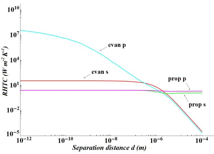
To calculate the RHTC, we replace Eqs. (1.16) into the expression given by Eqs. (1.13) to obtain the RHTC as function of the separation distance _{𝑑. By numerically calculating the obtained} equation, we plot in Fig. 1.6 the different contributions of the waves of s and p polarization to the RHTC.

Figure 1.6: Variation of the radiative heat transfer coefficient (contributions of the evanescent and propagative EM waves of s and p polarizations) between two semi-infinite 6H- SiC parallel

(31)

20

Fig. 1.6 shows the graphs of the contributions of the evanescent and propagative EM waves of

sand p polarization to the RHTC. We also plotted the total contribution which is the sum of all

the four contributions as to compare between the graphs.

From these graphs, we observe that the contributions of the propagative EM waves of both s and

p polarizations dominate at large distances and did not change a lot for submicronic distances as

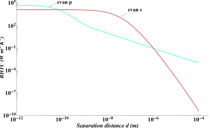
they saturate for small distances. Propagative waves dominate at large distances because in the far field the evanescent waves rapidly decrease as the separation distances is large compared to 𝜆𝑚𝑎𝑥, and by this the value of the RHTC is limited to the contribution of propagative waves and is somewhat less than the value _4𝜎𝑇3 [9,10,20,21] which is the standard heat transfer coefficient for a blackbody. This is due to the fact that SiC is highly absorbent over a wide spectral range, except around _{10.6µ𝑚 where it is reflective. We also notice in Fig. 1.6 that the contribution of} the p polarized propagative waves gives values slightly higher than those of the s polarized propagative waves; this is explained as being due to the existence of the Brewster angle for which the reflection contribution of the p polarized waves is zero and thus allowing greater absorption.

To better interperet the obtained results, it is essential to emphasize that the heat transfer is mainly governed by the mean energy of an oscillator at frequency _{𝜔 and at temperature T and} by the density of EM states. It follows that the propagative contributions of s and p polarizations did not change significantly at small distances because the density of EM propagative states at these distances scales does not change significantly [21].

Regarding the contributions of the evanescent EM waves, we observe that at large distances they are negligible compared to the contributions of the propagative waves. This is due to the fact that the evanescent waves decay exponentially away from the surface so that at large distance their decaying rate is large. At sub-wavelength distances, evanescent waves decaying rate is small so that these waves can tunnel between the surfaces and their contributions to the RHTC become dominant. The evanescent contribution of s polarization shows negligible contribution in the far-field and saturates when the distance is smaller than the skin depth [52].This contribution of the

s-polarized evanescent waves could be attributed to the presence of eddy currents on a typical

distance equal to the skin depth. When the distance is smaller than the skin depth, the transfer saturates to a value given by a distribution of the current in all the material.

To better understand the results obtained for the evanescent waves contributions it is important to highlight the role of the imaginary part of the reflection factor in the RHTC equation. From Eqs. (1.13) we notice that the evanescent term is proportional to the square of the imaginary part of the reflection factor which leads to the importance of studying the variation of