Universit´e de Montr´eal
ESSAYS IN EMPIRICAL FINANCE
par Magnim Farouh
D´epartement de sciences ´economiques Facult´e des arts et des sciences
Th`ese pr´esent´ee `a la Facult´e des ´etudes sup´erieures et postdoctorales en vue de l’obtention du grade de PhilosophiæDoctor (Ph.D.)
en Sciences ´economiques
Aoˆut, 2020
c
Universit´e de Montr´eal
Facult´e des ´etudes sup´erieures et postdoctorales
Cette th`ese intitul´ee:
ESSAYS IN EMPIRICAL FINANCE
pr´esent´e par: Magnim Farouh
a ´et´e ´evalu´ee par un jury compos´e des personnes suivantes: Guillaume Sublet Pr´esident-rapporteur
Ren´e Garcia Directeur de recherche Vasia Panousi Co-directrice de recherche Marine Carrasco Membre du jury
Ruslan Goyenko Examinateur externe
... Repr´esentant du doyen de la FAS
R´
esum´
e
Cette th`ese comporte trois chapitres dans lesquels j’´etudie les coˆuts de transaction des actions, les anomalies en finance et les activit´es du syst`eme bancaire parall`ele.
Dans le premier chapitre (co-´ecrit avec Ren´e Garcia), une nouvelle fa¸con d’estimer les coˆuts de transaction des actions est propos´ee. Les coˆuts de transaction ont diminu´e au fil du temps, mais ils peuvent augmenter consid´erablement lorsque la liquidit´e de financement se rar´efie, lorsque les craintes des investisseurs augmentent ou lorsqu’il y a d’autres frictions qui empˆechent l’arbitrage. Nous estimons dans ce chapitre les ´ecarts entre les cours acheteur et vendeur des actions de milliers d’entreprises `a une fr´equence journali`ere et pr´esentons ces mouvements importants pour plusieurs de ces ´episodes au cours des 30 derni`eres ann´ees. Le coˆut de transaction des trois quarts des actions est fortement impact´e par la liquidit´e de financement et augmente en moyenne de 24 %. Alors que les actions des petites entreprises et celles des entreprises `a forte volatilit´e ont des coˆuts de transaction plus ´elev´es, l’augmentation relative des coˆuts de transaction en temps de crise est plus prononc´ee pour les actions des grandes entreprises et celles des entreprises `a faible volatilit´e. L’´ecart entre les coˆuts de transaction respectifs de ces groupes de qualit´e ´elev´ee et qualit´e faible augmente ´egalement lorsque les conditions financi`eres se d´et´eriorent, ce qui prouve le ph´enom`ene de fuite vers la qualit´e. Nous avons construit des portefeuilles bas´es sur des anomalies et avons estim´e leurs “alphas” ajust´es pour les coˆuts de r´e´equilibrage sur la base de nos estimations des coˆuts de transaction pour montrer que toutes les strat´egies sont soit non rentables soit perdent de l’argent, `a l’exception de deux anomalies: le “prix de l’action” et la “dynamique du secteur industriel”.
Dans le deuxi`eme chapitre, j’´etudie comment la popularit´e des anomalies dans les revues scientifiques sp´ecialis´ees en finance peut influer sur le rendement des strat´egies bas´ees sur ces anomalies. J’utilise le ton du r´esum´e de la publication dans laquelle une anomalie est discut´ee et le facteur d’impact de la revue dans laquelle cette publication a paru pour pr´evoir
le rendement des strat´egies bas´ees sur ces anomalies sur la p´eriode apr`es publication. La principale conclusion est la suivante: lorsqu’une anomalie est discut´ee dans une publication dont le r´esum´e a un ton positif, et qui apparaˆıt dans une revue avec un facteur d’impact sup´erieur `a 3 (Journal of Finance, Journal of Financial Economics, Review of Financial Studies), cette anomalie est plus susceptible d’attirer les investisseurs qui vont baser leurs strat´egies sur cette anomalie et corriger ainsi la mauvaise ´evaluation des actions.
Le troisi`eme chapitre (co-´ecrit avec Vasia Panousi ) propose une mesure de l’activit´e bancaire parall`ele des entreprises op´erant dans le secteur financier aux ´Etats-Unis. `A cette fin, nous utilisons l’analyse de donn´ees textuelles en extrayant des informations des rap-ports annuels et trimestriels des entreprises. On constate que l’activit´e bancaire parall`ele ´
etait plus ´elev´ee pour les “Institutions de d´epˆot”, les “Institutions qui ne prennent pas de d´epˆot” et le secteur “Immobilier” avant 2008. Mais apr`es 2008, l’activit´e bancaire parall`ele a consid´erablement baiss´e pour toutes les firmes op´erant dans le secteur financier sauf les “Institutions non d´epositaires”. Notre indice du syst`eme bancaire parall`ele satisfait certains faits ´economiques concernant le syst`eme bancaire parall`ele, en particulier le fait que les poli-tiques mon´etaires restrictives contribuent `a l’expansion du syst`eme bancaire parall`ele. Nous montrons ´egalement avec notre indice que, lorsque l’activit´e bancaire parall`ele des 100 plus grandes banques augmente, les taux de d´elinquance sur les prˆets accord´es par ces banques augmentent ´egalement. L’inverse est observ´e avec l’indice bancaire traditionnel: une aug-mentation de l’activit´e bancaire traditionnelle des 100 plus grandes banques diminue le taux de d´elinquance.
Mots cl´es: Coˆuts de transaction, Anomalie, Liquidit´e de financement, ´Echantillonnage de Gibbs, Facteur de Bayes, Analyse de donn´ees textuelles, Facteur d’impact d’un journal, Activit´e bancaire parall`ele
Abstract
This thesis has three chapters in which I study transaction costs, anomalies and shadow banking activities.
In the first chapter (co-authored with Ren´e Garcia) a novel way of estimating trans-action costs is proposed. Transtrans-action costs have declined over time but they can increase considerably when funding liquidity becomes scarce, investors’ fears spike or other frictions limit arbitrage. We estimate bid-ask spreads of thousands of firms at a daily frequency and put forward these large movements for several of these episodes in the last 30 years. The transaction cost of three-quarters of the firms is significantly impacted by funding liquidity and increases on average by 24%. While small firms and high volatility firms have larger transaction costs, the relative increase in transaction costs in crisis times is more pronounced in large firms and low-volatility firms. The gap between the respective transaction costs of these high- and low-quality groups also increases when financial conditions deteriorate, which provides evidence of flight to quality. We build anomaly-based long-short portfolios and esti-mate their alphas adjusted for rebalancing costs based on our security-level transaction cost estimates to show that all strategies are either unprofitable or lose money, except for price per share and industry momentum.
In the second chapter I study how the popularity of anomalies in peer-reviewed finance journals can influence the returns on these anomalies. I use the tone of the abstract of the publication in which an anomaly is discussed and the impact factor of the journal in which this publication appears to forecast the post-publication return of strategies based on the anomaly. The main finding is the following: when an anomaly is discussed in a positive tone publication that appears in a journal with an impact factor higher than 3 (Journal of Finance, Journal of Financial Economics, Review of Financial Studies), this anomaly is more likely to attract investors that are going to arbitrage away the mispricing.
banking activity of firms operating in the financial industry in the United States. For this purpose we use textual data analysis by extracting information from annual and quarterly reports of firms. We find that the shadow banking activity was higher for the “Depository Institutions”, “Non depository Institutions” and the “Real estate” before 2008. But after 2008, the shadow banking activity dropped considerably for all the financial companies except for the “Non depository Institutions”. Our shadow banking index satisfies some economic facts about the shadow banking, especially the fact that contractionary monetary policies contribute to expand shadow banking. We also show with our index that, when the shadow banking activity of the 100 biggest banks increases, the delinquency rates on the loans that these banks give also increases. The opposite is observed with the traditional banking in-dex: an increase of the traditional banking activity of the 100 biggest banks decreases the delinquency rate.
Keywords: Transaction cost, Anomaly, Funding liquidity, Gibbs sampling, Bayes factor, Textual analysis, Journal impact factor, Shadow banking, Term frequency - Inverse document frequency.
Table des mati`
eres
Table of contents
R´esum´e . . . iv
Abstract . . . vi
Table des mati`eres / Table of contents . . . x
Liste des tableaux / List of Tables . . . xiii
Liste des Figures / List of Figures . . . xvi
D´edicace / Dedication . . . xvii
Remerciements / Acknowledgements . . . xviii
Avant-propos / Foreword 1 1 Financial Risks, Transaction costs and Performance of Anomalies 3 1.1 Introduction . . . 3
1.2 Methodology . . . 8
1.2.1 Measuring the Effective Bid-ask Spread from Daily Prices . . . 9
1.2.2 The Hasbouck Model with Financial Risk . . . 11
1.2.3 Estimation of the effective bid-ask spread with financial risk . . . 11
1.3 Data Construction . . . 14
1.4 Transaction Costs with Funding Liquidity Risk . . . 15
1.4.1 Average Transaction Costs . . . 16
1.4.2 The Dynamics of Transaction Costs . . . 17
1.4.3 Transaction Costs and other Financial Risk Measures . . . 21
1.5.1 Gross Returns and Net Returns of Anomalies . . . 24
1.5.2 Performance of Long-short Strategies . . . 25
1.6 Robustness Check: the Transaction-cost Model of Lesmond, Ogden and Trzcinka (LOT) (1999) . . . 27
1.6.1 Specification of the LOT Model . . . 27
1.6.2 Estimation of the LOT Model . . . 28
1.6.3 The LOT Model with Funding Liquidity . . . 30
1.6.4 Estimated Transaction Costs with the LOT and LOT-FL Models for Anomaly-based Portfolios . . . 32
1.6.5 Performance of Long-short Strategies with the LOT Models . . . 33
1.7 Conclusion . . . 34
Tables and Figures of Chapter 1 . . . 35
Appendices for Chapter 1 (A) 62 Anomalies . . . 62
Additional Tables and Figures . . . 68
2 Journal Picking for Better Returns 74 2.1 Introduction . . . 74
2.2 Methodology . . . 78
2.2.1 Publications that discuss an Anomaly . . . 78
2.2.2 The Tone Index and the Journal Impact Factor . . . 79
2.2.3 Empirical Analyses . . . 81
2.3 Data . . . 83
2.4 Results . . . 83
2.4.1 Tone Index and Journal Impact Factor . . . 83
2.4.2 Portfolio Returns Relative to End-of-Sample and First Publication Dates 84 2.4.3 Forecasting the Return of Anomaly-based Strategies . . . 85
2.5.1 Effect of Publications from Journal of Banking & Finance . . . 88
2.5.2 Effect of Transaction Costs . . . 88
2.6 Conclusion . . . 90
Tables and Figures of Chapter 2 . . . 91
Appendices for Chapter 2 (B) 106 Anomalies . . . 106
Transaction cost calculation . . . 110
3 Shadow Banking in the US 111 3.1 Introduction . . . 111
3.2 The US Banking System . . . 115
3.2.1 Traditional Banking . . . 115
3.2.2 Shadow Banking . . . 116
3.3 Data . . . 116
3.4 Methodology . . . 117
3.4.1 Shadow Banking Word List . . . 118
3.4.2 TF-IDF Weighting Scheme . . . 118
3.5 Shadow-Banking Activity Index . . . 120
3.5.1 Descriptive Analysis . . . 120
3.5.2 Co-movement with Securitisation . . . 121
3.5.3 Monetary Policy and Funding Liquidity . . . 122
3.6 Shadow-Banking Activity Index and Delinquency Rates . . . 123
3.7 Conclusion . . . 124
Tables and Figures of Chapter 3 . . . 126
Appendices for Chapter 3 (C) 141 Dictionary of Shadow Banking words . . . 141
Liste des tableaux
List of Tables
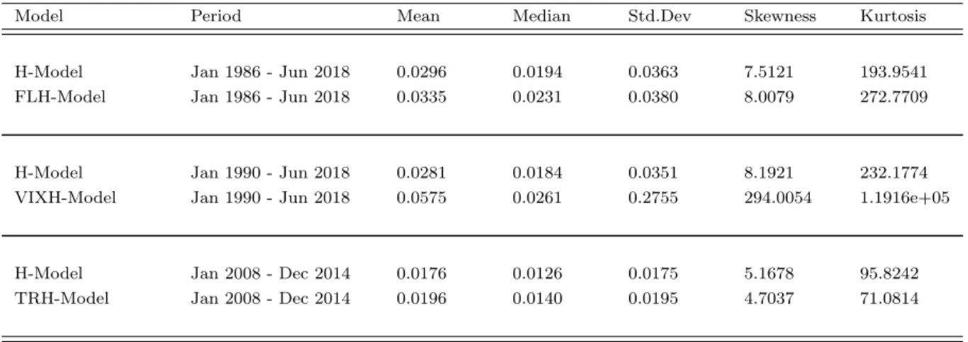
1.1 Summary statistics for the estimated transaction costs with each H-Model . . . 36 1.2 Average H-Model and FLH-Model transaction costs for
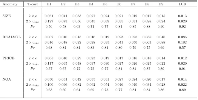
anomaly-based decile portfolios . . . 37 1.3 FLH-Model: Transaction costs and flight to quality . . . 40 1.4 Average H-Model and VIXH-Model transaction costs for
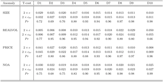
anomaly-based decile portfolios . . . 41 1.5 Average H-Model and TRH-Model transaction costs for
anomaly-based decile portfolios . . . 42 1.6 Alphas (in %) of anomaly portfolios with H-Model and FLH-Model
transaction costs (January 1986 to June 2018) . . . 43 1.7 Alphas (in %) of anomaly portfolios with H-Model and VIXH-Model
transaction costs (January 1990 to June 2018) . . . 45 1.8 Alphas (in %) of anomaly portfolios with H-Model and TRH-Model
transaction costs (January 2008 to December 2014) . . . 47 1.9 Average LOT selling and buying transaction costs for anomaly-based
decile portfolios . . . 49 1.10 Alphas (in %) of anomaly portfolios with Model and
LOT-Model plus funding liquidity (FLLOT-LOT-Model) transaction costs (Jan-uary 1986 to June 2018) . . . 54 1.11 VIXH-Model: Transaction costs and flight to quality . . . 68
1.12 TRH-Model: Transaction costs and flight to quality . . . 69
2.1 Summary Statistics by Journal . . . 92
2.2 Anomalies and Average Tone index . . . 93
2.3 Anomalies and JIF . . . 94
2.4 Regression of portfolio Returns on sample dummy and on post-publication dummy . . . 95
2.5 Regression of post publication returns on publication tone and jour-nal impact factor . . . 96
2.6 Regression of average post publication return on publication tone (number of positive words minus number of negative words in pub-lication abstract and journal impact factor . . . 97
2.7 Regression of average post publication return on publication tone and journal impact factor . . . 98
2.8 Regression of average post publication return on publication tone (%age of positive words) and journal impact factor . . . 99
2.9 Regression of average post publication return on publication tone (%age of positive words minus %age of negative words) and journal impact factor . . . 100
2.10 Regression of post publication returns on publication tone and jour-nal impact factor considering only Jourjour-nal of Banking and Finance 101 2.11 Regression of post publication returns on transaction cost, publi-cation tone and journal impact factor considering only Journal of Banking and Finance . . . 102
3.1 Number of reports by SIC code . . . 127
3.2 Number of reports by State . . . 128
3.3 Monetary policy, Shadow Banking Index and Traditional Banking Index . . . 129
3.4 100 Biggest bank in US as of December 2019 . . . 130
Liste des Figures
List of Figures
1.1 Proportion of funding liquidity t-cost for small firms and big firms 4 1.2 Transaction costs increase from H-Model to FLH-Model and TED
spread . . . 56 1.3 Dynamics of transaction costs from H-Model and FLH-Model for
COCA COLA CO . . . 57 1.4 Dynamics of transaction costs from H-Model and FLH-Model for
ROCKY MOUNTAIN CHOCOLATE FACTORY . . . 57 1.5 Dynamics of transaction costs from H-Model and FLH-Model for
small firms . . . 58 1.6 Dynamics of transaction costs from H-Model and FLH-Model for
big firms . . . 58 1.7 Dynamics of transaction costs from H-Model and FLH-Model for
high-volatility stocks . . . 59 1.8 Dynamics of transaction costs from H-Model and FLH-Model for
low-volatility stocks . . . 59 1.9 Separating the transaction cost into its fixed component and its
time-varying TED-spread component . . . 60 1.10 Dynamics of transaction costs from H-Model and VIXH-Model for
small, big, low-volatility, and high-volatility firms . . . 60 1.11 Dynamics of transaction costs from H-Model and TRH-Model for
1.12 Dynamics of transaction costs from H-Model and FLH-Model for Losers . . . 70 1.13 Dynamics of transaction costs from H-Model and FLH-Model for
Winners . . . 70 1.14 Dynamics of transaction costs from H-Model and VIXH-Model for
COCA COLA CO . . . 71 1.15 Dynamics of transaction costs from H-Model and VIXH-Model for
ROCKY MOUNTAIN CHOCOLATE FACTORY . . . 71 1.16 Dynamics of transaction costs from H-Model and TRH-Model for
COCA COLA CO . . . 72 1.17 Dynamics of transaction costs from H-Model and TRH-Model for
ROCKY MOUNTAIN CHOCOLATE FACTORY . . . 72 1.18 Separating the transaction cost into its fixed component and its
time-varying TED-spread component: small firms . . . 73 1.19 Separating the transaction cost into its fixed component and its
time-varying TED-spread component: large firms . . . 73 2.1 Evolution of Number of publications that discuss anomalies . . . 103 2.2 Evolution of Percentage of publications that discuss anomalies . . . 103 2.3 Scatter plot between post publication average anomaly return and
publication tone . . . 104 2.4 Evolution of beta1, beta2 and beta3 with respect to q . . . 105
3.1 Channels of Financial Intermediation (Luttrell et al. [2012]) . . . 135 3.2 Average Shadow banking activity (from 10-Ks) by SIC code . . . . 135 3.3 Evolution from 1994 to 2019 of shadow banking (from 10-Ks) . . . 136 3.4 Evolution from 1994 to 2019 of shadow banking by the state in which
the firm is located (from 10-Ks) . . . 137 3.5 Evolution by type of financial company from 1994 to 2019 of shadow
3.6 Shadow banking and Total Real Estate Loans Owned and Securitized by Finance Companies . . . 139 3.7 Shadow banking and Money Market funds total financial assets . . 140
`
Remerciements
Acknowledgements
J’aimerais tout d’abord remercier mon directeur de recherche, Ren´e Garcia, pour la confiance qu’il a plac´ee en moi en acceptant de m’encadrer mais surtout, pour sa disponibilit´e, son suivi continu, ses nombreux conseils et sa gentillesse. Merci Ren´e, d’avoir ´et´e mon mentor pendant toutes ces ann´ees.
Je remercie par ailleurs Vasia Panousi, pour tout le soutien qu’elle m’a apport´e dans les derni`eres ann´ees de mes ´etudes doctorales. Elle est le professeur avec qui j’ai appris les techniques d’analyse textuelle qui m’ont beaucoup servi dans ma th`ese.
Toute ma gratitude `a William Mccausland pour sa disponibilit´e, `a Benoˆıt Perron pour ses remarques et conseils, `a tous les professeurs du d´epartement d’´economie de l’Universit´e de Montr´eal, ainsi qu’`a l’ensemble du personnel administratif dudit d´epartement.
Mes sinc`eres remerciements `a tous les doctorants en ´economie de l’Universit´e de Montr´eal, et plus particuli`erement `a mes camarades de promotion Fatim, Idriss, Lionel, Lucienne, Marl`ene, N’Golo, et Samuel ainsi qu’`a F´elicien, Kokouvi, et Souleymane. Merci pour votre pr´esence et vos encouragements. Je remercie par ailleurs mon grand fr`ere Germain, mon p`ere et ma m`ere pour leurs soutien et conseils dans les moments de doute.
Je tiens enfin `a remercier le D´epartement de sciences ´economiques de l’Universit´e de Montr´eal, la Facult´e des arts et des sciences, le Centre Inter-universitaire de Recherche en Economie Quantitative (CIREQ) et la Facult´e des ´etudes sup´erieures et postdoctorales, pour leur soutien financier et logistique.
Avant-propos
Foreword
Expliquer l’´evolution des rendements des actifs financiers a toujours ´et´e une pr´eoccupation pour les chercheurs en finance. Sharpe[1964] etLintner[1965] ont pos´e les bases de ce qui est aujourd’hui un champ de recherche florissant en ´evaluation des actifs financiers: l’explication des rendements `a partir d’un nombre r´eduit de facteurs observ´es. Le CAPM a ´et´e le premier mod`ele de ce genre, et a ´et´e suivi par une multitude de mod`eles `a facteurs dont les plus populaires sont en particulier le mod`ele de Fama-French, le CAPM intertemporel, le CAPM conditionnel, et le mod`ele de Carhart, etc..
Une anomalie est d´efinie comme toute variable qui procure une pr´edictibilit´e inconsis-tante avec le mod`ele d’´evaluation d’actifs financiers consid´er´e (CAPM, mod`eles Fama-French ou autre). Ces derni`eres ann´ees, les chercheurs en finance et comptabilit´e ont publi´e dans les revues de finance et comptabilit´e plus de 150 anomalies. Les anomalies ont donn´e aux investisseurs l’opportunit´e de pouvoir construire des strat´egies pour pouvoir r´ealiser des prof-its. Ces strat´egies consistent `a construire des portefeuilles dynamiques d’actions expos´es `a l’anomalie. Le dynamisme de ces portefeuilles requiert des ajustements fr´equents qui font que les investisseurs font face `a des coˆuts de transaction sur le march´e financier, surtout en p´eriode de crise de liquidit´e financi`ere.
Pour pouvoir profiter d’une anomalie, l’investisseur doit d’abord ˆetre au courant qu’une telle anomalie existe et pour cela il doit s’informer en se renseignant sur les avanc´ees dans le domaine de la recherche acad´emique en finance. Une fois qu’il est au courant de l’anomalie, l’investisseur doit cr´eer le portefeuille dynamique bas´e sur cette anomalie. Avoir une bonne mesure des coˆuts de transaction sur le march´e financier est ainsi vital pour un investisseur qui aimerait baser ses strat´egies sur les anomalies, ´etant donn´e que maintenir un porte-feuille constamment expos´e `a l’anomalie n´ecessite des ajustements impliquant ainsi des coˆuts de transaction. Une bonne mesure du coˆut de transaction d’une action devrait inclure les
´
el´ements relatifs `a cette action, mais aussi les ´el´ements relatifs `a l’environnement global du march´e financier et ´economique.
L’environnement ´economique et financier d´epend fortement des activit´es bancaires. Le secteur bancaire procure aux agents ´economiques (dont ceux qui investissent sur le march´e financier) du financement pour pouvoir mener leurs activit´es. Dans le secteur bancaire, nous distinguons deux types de banques : les banques traditionnelles qui re¸coivent des d´epˆots et accordent des prˆets aux m´enages et aux entreprises, sous la supervision des r´egulateurs et des banques centrales; les banques parall`eles, par contre sont des interm´ediaires financiers qui facilitent la cr´eation de cr´edit dans l’´economie via la titrisation des actifs, sans accepter de d´epˆots et sans faire l’objet d’une surveillance r´eglementaire. Quelques exemples de banques parall`eles incluent les fonds sp´eculatifs, les compagnies d’assurance et les soci´et´es d´eriv´ees. Vu l’importance de leurs activit´es durant la crise financire de 2008, les banques parall`eles semblent ˆetre celles qui comportent le plus de risques. Avoir un bon suivi des activit´es des banques parall`eles est donc tr`es important pour les d´ecideurs publics.
Les trois articles de cette th`ese s’inscrivent dans une logique de d´eveloppement de nou-veaux outils permettant de:
• mesurer les coˆuts de transaction des actions et l’effet de ces coˆuts sur les profits de strat´egies bas´ees sur les anomalies;
• voir comment les investisseurs s´electionnent les anomalies en fonction des journaux dans lesquels ces anomalies sont publi´ees;
• avoir une nouvelle mesure des activit´es du secteur bancaire parall`ele.
Dans le premier chapitre de cette th`ese, une estimation des coˆuts de transactions des ac-tifs financiers prenant en compte les frictions qui peuvent constituer un frein pour l’arbitrage, est propos´ee. Le deuxi`eme chapitre montre comment la popularit´e des anomalies publi´ees dans les revues scientifiques sp´ecialis´ees en finance et la qualit´e de ces revues peuvent influer sur le rendement des strat´egies bas´ees sur ces anomalies. Le troisi`eme chapitre, enfin, propose une mesure des activit´es bancaires parall`eles bas´ee sur les rapports annuels des firmes qui op`erent dans le secteur financier aux ´Etats-Unis.
Chapter 1
Financial Risks, Transaction costs and
Performance of Anomalies
1.1
Introduction
Algorithmic trading is everywhere present in financial markets. While the trading rules are set by fund managers, their execution is fully automatized1. A positive effect of this automation
is the reduction of transaction costs. Machines help reduce the part of transaction costs that is related to a firm’s specific information since news are instantly reflected in its security price. However, transaction costs of firms may be also affected by aggregate market conditions such as limited funding liquidity, heightened investors’ fears or other frictions that limit arbitrage. The main focus of this paper is to provide estimates of transaction costs that include the cost of these market frictions. We incorporate measures of financial risks such as funding liquidity or tail risk in the current estimation procedures of bid-ask spreads. A second objective is to measure the impact of these time-varying, market-based transaction costs on the returns of long-short strategies that arbitrageurs are pursuing by building portfolios sorted on firm characteristics. We assess what remains of the alpha of dynamic strategies based on so-called anomalies once we incorporate the additional rebalancing costs due to aggregate frictions.
1According to a recent article in The Economist, funds run by computers that follow rules set by humans
account for 35% of America’s stock market, 60% of institutional equity assets and 60% of trading activity. According to Deutsche Bank, 90% of equity-futures trades and 80% of cash-equity trades are executed by algorithms without any human input.
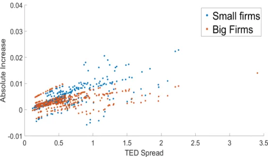
Figure 1.1: Proportion of funding liquidity t-cost for small firms and big firms
In our model, the transaction cost is written as an affine function of the financial risk measure: t-cost = c0 + c1 × financial-risk. For the estimation we use the Gibbs Sampling
method of Hasbrouck[2004] and Hasbrouck[2009]. Once we have the estimates of c0 and c1
for a given stock and a given year, we can compute the round-trip transaction cost for this stock, for a given day t, by t-costt= 2 × (c0+ c1× financial-riskt). To test if the financial risk
variable is statistically relevant for estimating the transaction cost we compute the Bayes factor between the Hasbrouck [2009] model (hereafter H-model) and the extended model including the financial risk variable (hereafter FLH-model for funding liquidity, TRH-model for tail risk and VIX-H model for the VIX).
Our empirical results support funding liquidity as an important factor in the estimation of transaction costs. To illustrate the role played by funding conditions especially in crisis periods, Figure 1.1 plots the time series of the proportion of the transaction costs due to funding liquidity for large and small firms. For each big financial market event between 1986 and 2018, the proportion jumps to about 60-70 % for large firms. Overall, large firms are relatively more impacted by funding conditions than small firms since their transaction costs are small in normal times. However, in the 2008 financial crisis that raised considerably liquidity risk, the proportion for small and large firms are about the same. Over the period
from January 1986 to June 2018, we find that there is more evidence for the FLH-Model against the H-Model for 73% of firm-years. Estimated transaction costs are in average 24% higher for the FLH-Model compared to the H-Model. The tail risk and VIX variables are also important in the estimation of transaction costs. We find with the Bayes factor that, there is more evidence for the TRH-Model and the VIX-H model against the H-Model respectively for 86% of firm-years and 74% of firm-years. With respect to the H-model, the estimated transaction costs are 19% and 95% higher for the TRH- and VIX-H models respectively.
We also investigate whether the estimated transaction costs reflect flight to quality. The quality of a particular stock is positively related to the size of the firm (Lang and Lundholm [1993]) and negatively related to the stock’s volatility (Brunnermeier and Pedersen [2009]). We will say that there is evidence for flight to quality if the differential in transaction costs between high and low quality stocks increases when the financial risk increases. We find that the differentials in transaction costs between small and large firms and high- and low-volatility firms increase when the financial risk increases.
The estimated transaction costs are also used to assess the after-trading-cost perfor-mance of long-short anomaly-based portfolios. The latter are constructed for a set of anoma-lies considered one at a time. Each month, stocks are ranked based on the value of the anomaly. Stocks are then grouped into deciles. The long-short portfolio is then obtained by going long on the stocks in the highest decile and short on the stocks in the lowest decile or inversely, depending on the anomaly2. Given the way the portfolios are built, each month or each year depending on the trading frequency, the stocks included in a given decile are not necessarily the same as in the previous month or year. Therefore, to stay exposed to the anomaly, the portfolios need to be rebalanced and transaction costs are incurred. We find that a proper accounting of the adjusted transaction costs for financial risks eliminates the profits of a large number of anomaly-based long-short portfolios.
For robustness purposes, we also consider the estimation of transaction costs with the model of Lesmond et al. [1999]. This model requires only the time series of daily security returns to endogenously estimate the effective transaction costs for any firm, exchange, or time period. The feature of the data that allows for the estimation of transaction costs is the incidence of zero returns. We introduce funding liquidity in this model and perform a likelihood ratio test with a model without frictions. The model with funding liquidity is
2Let us cite two examples. For momentum, the portfolio is obtained by going long on the stocks in the
highest decile and short on those in the lowest decile. For size, it is the reverse. The portfolio is long on stocks in the lowest decile and short on stocks in the highest decile.
preferred to the model without funding liquidity for a third of the firms.
The main objectives of the paper are motivated by two recent contributions to the litera-ture on transaction costs. Weller[2019] uses equity bid-ask spreads at high-frequency to infer a measure of tail risk, while Patton and Weller[2019] introduce market liquidity and funding liquidity variables to determine whether trading strategies based on some characteristics are implementable in practice. They better capture the price impact of trading strategies in large portfolios compared to Novy-Marx and Velikov [2016].
Our paper differs from this recent literature both in its methodology and scope. To measure the bid-ask spread of individual securities, we extend the model ofHasbrouck[2009] by adding financial risk variables to the market return factor. Our main application is based on the TED spread (short-term LIBOR minus short Treasury rate) that is used to measure funding liquidity cost. We also consider for robustness purposes the measure of tail risk proposed by Weller [2019] and the VIX to capture liquidity frictions at the aggregate level.
Adding these variables to the measure of transaction costs is supported theoretically. Brunnermeier and Pedersen [2009] propose a theoretical model that shows that transaction costs depend on funding liquidity. Since Weller[2019] proposes a measure of tail risk based on the cross-section of bid-ask spreads, such a measure can help recover effective transaction costs. This is explained by the fact that liquidity providers, in moments of tight funding constraints or extreme events require a high compensation leading to high transaction costs. The VIX could also affect transaction costs because higher volatility tightens funding con-straints of market makers and thereby reduces their liquidity-provision capacity (Gromb and Vayanos [2002], Brunnermeier and Pedersen [2009],Nagel [2012]).
The rest of the paper is structured as follows. After reviewing the literature on the measurement of transaction costs, we describe in Section 1.2 the estimation methodology of transaction costs based on the model of Hasbrouck [2009] and the extensions made to include measures of financial risks. We also explain how the new model including financial risk is compared to the basic Hasbrouck model. Section 1.3 describes the data used for the estimation. Section 1.4 presents the results of the transaction costs estimation for the various models. Robustness checks are reported in Section 1.5. In Section 1.6 the perfor-mances of anomaly-based strategies are computed after taking in account the transaction costs augmented by financial frictions. Section 1.7 concludes.
Related Literature
The most direct way to measure transaction costs is to take the bid-ask spread plus com-missions. However, according to Ng et al. [2008], the bid-ask spread underestimates the real transaction costs because it does not take in account relevant elements such as price impact or opportunity costs. According to Roll[1984], commissions depend on a number of hard-to-quantify factors (such as the transaction size, the amount of business done by the investor, and the time of day or year) given that they are negotiated. Grossman and Miller [1988] argue that, for a given trade, it is unlikely that the seller and the buyer arrive at the same time on the market and thus the spread cannot serve as the measure of the transaction cost. Another issue with the bid-ask spread is that it is not always available for all firms and time periods where security returns exist.
To overcome the issues associated with a direct measure of bid-ask spreads based on trades and quotes, Roll [1984] proposed a model to estimate the transaction costs by a so-called effective bid-ask spread. The suggested measure for the effective bid-ask spread is based on the fact that transaction costs induce negative serial dependance in successive observed market price changes. However, it is not always the case that this covariance is negative in the data. To overcome this issue, Hasbrouck [2004] proposes a Gibbs sampling estimate ofRoll [1984] model that is based on daily closing prices. Hasbrouck[2009] extends the Hasbrouck [2004] model by including a market return factor in the estimation equation and shows that the estimated effective spreads have a 96.5% correlation with the ones estimated from actual trades from the trade and quote (TAQ) dataset. Goyenko et al. [2009] confirms that the effective bid-ask spread is a good proxy for the bid-ask spreads estimated with intra-daily trade-and-quote data.
The Bayesian procedure proposed byHasbrouck[2009] necessitates long time series, leav-ing some firms without a transaction cost estimate. A solution is to rely on proxies.3 Novy-Marx and Velikov [2016] use the fact that market capitalization and idiosyncratic volatility explain around 70% of the cross section of transaction costs to assign transaction costs to stocks for which the model proposed by Hasbrouck [2009] could not deliver an estimate.
Lesmond et al. [1999] propose a model of security returns that avoids the limitations of
3Karpoff and Walkling[1988] andBhushan[1994] use price, trading volume, firm size, and the number of
shares outstanding, variables assumed to be negatively related to transaction costs. Of course, proxy variables may capture effects that are not due to transaction costs and cannot be used to compute net returns of a portfolio.
the transaction cost proxies. The effect of transaction costs is modeled through the incidence of zero returns. If the value of the information signal is insufficient to exceed the costs of trading, then the marginal investor will not trade, causing a zero return. The estimates from this model are the marginal traders effective transaction costs. Lesmond et al.[2004] use this methodology to compute the after-transaction-cost returns of different momentum portfolios to prove that the profits from momentum strategies are illusory.
The implementation costs of financial market anomalies has also been studied recently byPatton and Weller[2019]. They estimate the transaction costs of mutual funds strategies by relying onCorwin and Schultz[2011]’s methodology to estimate bid-ask spreads based on daily high and low prices.
Our paper is also related to the literature on the link between market liquidity (as measured by the bid-ask spread) and financial risk measures such as funding liquidity (Gromb and Vayanos [2002], Brunnermeier and Pedersen [2009] and Kondor and Vayanos [2019]), the VIX (Nagel [2012]) or tail risk (Weller [2019]). Aragon and Strahan [2012] document empirically the relationship between funding liquidity and market liquidity by linking the market liquidity of stocks held by hedge funds exposed to Lehman Brothers to shocks to funding liquidity during the bankruptcy.
Our paper also relates to the large literature about the limits of arbitrage (Shleifer and Vishny [1997], Geanakoplos [2010], Gromb and Vayanos [2010]). Tight funding conditions increase transaction costs and therefore prevent arbitrageurs from taking advantage of mis-priced assets.
1.2
Methodology
To overcome the issues associated with a direct measure of bid-ask spreads based on trades and quotes, Roll [1984] proposed a model to estimate the transaction costs by a so-called effective bid-ask spread from daily security prices. In this section we describe the estimation procedures to arrive at a measure of transaction costs that fluctuates with a measure of financial risk. Since it is a Bayesian estimation procedure we provide all the steps of the Gibbs-sampling algorithm for the various parameters of the model.
1.2.1
Measuring the Effective Bid-ask Spread from Daily Prices
To incorporate funding liquidity risk, volatility risk or tail risk into the measure of the effective bid-ask spreads of firms, we extend the Bayesian procedure of Hasbrouck [2009]. We start by describing the model of Roll [1984] on which the procedure is based, then the Bayesian estimation and finally the incorporation of the financial risk factor in the procedure.
a. The model of Roll (1984)
Transaction prices are composed of a random-walk and a noise, wherein the random-walk is the “efficient price” of security and the noise is the bid-ask spread, as follows:
mt = mt−1+ εt (1.1)
bt= mt− c (1.2)
at = mt+ c (1.3)
where mtis the efficient price’, btthe bid price and atthe ask price, all expressed in logarithms,
εt a random disturbance reflecting public information about the stock, and c is the
half-spread, presumed to reflect the quote-setter’s cost of market-making.
The model introduces a random indicator qt to capture the direction of the trade. It
takes the value one with probability 0.5 if the trade takes place at the ask, and minus one with probability 0.5 if it does at the bid.
If ptis the observed transaction price, equations (1.2) and (1.3) can be summarized with
the following equation: pt= mt+ c.qt. Therefore:
∆pt= c∆qt+ εt, (1.4)
which yields Cov(∆pt, ∆pt+1) = Cov(c.∆qt + εt, c.∆qt+1 + εt+1). In most
implementa-tions of the Roll model, it is assumed that the direction of the trade is independent of the efficient price movement i.e. qt is independent of εt. With this assumption, we
ob-tain Cov(∆pt, ∆pt+1) = c2.Cov(∆qt, ∆qt+1). Given that qt is equal to +1 or −1 with
equal probabilities, Cov(∆pt, ∆pt+1) = −c2. Therefore, the half-spread is equal to c =
p−Cov(∆pt, ∆pt+1).
daily changes in stock prices. Roll [1984] finds that auto-covariance estimates based on 21 daily returns are positive for almost half the cases. Harris [1990] studies the statistical properties of the Roll bid-ask spread estimator and shows that positive auto-covariances are more likely for low values of the spread.
Hasbrouck [2009] argues that another problem arises when there is no trade on a par-ticular day. When there is no trade on a parpar-ticular day, CRSP reports the midpoint of the closing bid and ask. If these days are retained in the sample, the estimated cost will generally be biased downward, because the midpoint realizations do not include the cost. If these days are dropped from the sample, heteroscedasticity may arise since the efficient price innovations may span multiple days.
b. The Bayesian procedure of Hasbrouck (2004, 2009)
To overcome this issue, Hasbrouck [2004] proposes a Bayesian approach. In this approach, Hasbrouck [2004] makes two key assumptions: the spread is positive and εtiid ∼ N (0, σε2).
The model parameter set is Θ = {σ2
ε, c}. Denote the prior parameter density as π(Θ). The
posterior is given by f (Θ/p) = f (p/Θ).π(Θ)f (p) , where p = {p1, p2, ..., pT} denotes the vector of
observed prices.
This posterior cannot be directly evaluated because the data likelihood function f (Θ/p) involves the unobserved q = {q1, q2, ..., qT}. The problem is solved by considering f (Θ, q/p)
and then by integrating out the q. Hasbrouck [2004] uses a Markov-Chain Monte-Carlo (MCMC) approach for this purpose.
Hasbrouck [2009] extends the model by including a market return factor in the Roll model:
∆mt = βmrmt+ εt. (1.5)
Therefore, if we replace mt by pt+ c.qt, the observed price change is given by:
∆pt= c∆qt+ βmrmt+ εt. (1.6)
The assumption εt iid ∼ N (0, σε2) is maintained, while the new parameter set is Θ =
{σ2
ε, c, β}. The problem is solved by considering f (Θ, q/p.rm) and then by integrating out
1.2.2
The Hasbouck Model with Financial Risk
In the model of Hasbrouck [2009], the transaction cost of a firm for a time period (be it a month, a quarter or a year) is estimated from its daily returns. It means that the cost will be constant for each time period. Our contribution is to link the transaction cost to a financial risk measure and make it time-varying at the daily level.
1.2.3
Estimation of the effective bid-ask spread with financial risk
We write the transaction cost as an affine function of the financial risk measure F Rt. We
make the notation more precise than in the previous sections since we have to distinguish the time scales for the various coefficients and identify the firm since we will be forming anomaly portfolios in the second part of the paper.
mit= mit−1+ εit (1.7) pit= mit+ (ci0,tp+ ci1,tp.F Rt)qti, (1.8)
where mitis the underlying log efficient value, pitis the log trade price, qitis a random indicator for the direction of the trade that takes the value one (minus one) if the trade took place at the ask (bid), εit is a random disturbance reflecting public information about the stock, and ci
t = ci0,tp+ ci1,tp.F Lt is the effective cost of trading. The subscript t corresponds to the
daily frequency, while tp denotes the time period over which we estimate the transaction cost
(monthly or yearly). The coefficients c0,tp and c1,tp are two coefficients that are constant over
each period p but vary from period to period. The effective cost of trading for firm i will be time varying at the daily level. The number of firms will be different each day and will be denoted by nt.
By generalizing the previous equation to include a market return factor, as inHasbrouck [2009], we obtain the following equation:
∆pit= (ci0,tp+ ci1,tp.F Rt)∆qit+ β i
mrmt+ εit (1.9)
∆pit= (ci0,tp.∆qti+ ci1,tp.F Rt.∆qti+ β i
mrmt+ εit (1.10)
AsHasbrouck[2009], we need to follow a Bayesian approach to estimate this model since qti, the random indicator for the direction of the trade, is unknown. We also assume that εit is iid N (0, σ2
εi). The parameters that will be estimated are ci0, ci1, βmi and σ2εi.
a. Simulating the Coefficients in a Linear Regression
The standard Bayesian normal regression model is y = Xb + e where y is a column vector of n observations of the dependent variable, X is an (n × k) matrix of fixed regressors, b is a vector of coefficients, and the residuals are zero-mean multivariate normal e ∼ N (0, Ωe).
Given Ωe and a normal prior on b, b ∼ N (µb, Ωb), the posterior is b ∼ N (µ∗b, Ω∗b), where
µ∗b = (X0Ω−1e X + Ω−1b )−1(X0Ω−1e y + Ω−1b µb) and Ω∗b = (X0Ω−1e X + Ω −1 b )
−1.
In our framework, the linear regression we have is ∆pit= ci0.∆qti+ci1·F Rt·∆qti+βmi rmt+εit.
Non-negativity is imposed on ci0 and ci1 in order to keep the transaction cost ct= ci0+ c1· F Rt
positive, since any of the financial risk measures considered is positive.
b. Simulating the Error Covariance Matrix
We also make the same assumption for Ωe = σ2I than Hasbrouck [2009]. The prior
distri-bution for σ2 is an inverted gamma distribution: σ2 ∼ IG(α, β). The posterior distribution
will also be an inverted gamma σ2 ∼ IG(α∗, β∗), where α∗ = α + n 2 and β
∗ = [β−1+Pei 2]
−1.
c. Simulating the Trade Direction Indicators
The remaining step in the sampler involves drawing q = q1, ..., qT when c0, c1, βm, and σ2
are known. The procedure is the same as the one used in Hasbrouck [2009]. The procedure is sequential. The first draw is q1/q2, ..., qT, the second draw is q2/q1, q3, q4, ..., qT, the third
d. Steps of the Sampling Procedure
For the sampler, we follow the steps and simulation parameter choices used in Hasbrouck [2009].
• Step 0 (initialization). Although the limiting behavior of the sampler is invariant to starting values, “reasonable” initial guesses may hasten convergence. The trade direction indicators qtthat do not correspond to midpoint reports are set to the sign of
the most recent price change, with q1 set (arbitrarily) to +1 and those corresponding
to midpoint reports are set to 0; σ2
ε is initially set to 0.00044. No initial values are
required for c0, c1 and βm, as they are drawn first.
• Step 1. Based on the most recently simulated values for σ2
ε and the set of qt, compute
the posterior for the regression coefficients (c0, c1 and βm) and make a new draw.
• Step 2. Given c0, c1 and βm, and the set of qt, compute the implied εt, update the
posterior for σ2ε, and make a new draw.
• Step 3. Given c0, c1, βm and σ2ε , make draws for q1, q2, ..., qT. qt that correspond to
midpoint reports are not drawn and are equal to 0. Go to Step 1.
Each sampler is run for 1,000 sweeps.5 Of the 1,000 draws for each parameter, the first
200 are discarded to burn in the sampler by removing the effect of starting values. The average of the remaining 800 draws (an estimate of the posterior mean) is used as a point estimate of the parameter.
e. A Bayes Factor to compare the Extended Model with Financial Risk to the Hasbrouck Model
The Bayes factor is the ratio of the marginal likelihoods of both models. Let M1,i,y and M2,i,y
denote the marginal likelihoods of the Hasbouck model and the extended model, respectively, and D the data set. For a firm i and a year y, the ratio can be written as:
BFi,y = P (M2,i,y/D) P (M1,i,y/D) = P (M2,i,y).P (D/M2,i,y) P (M1,i,y).P (D/M1,i,y) (1.11)
4This roughly corresponds to a 30% annual idiosyncratic volatility
Once again, the presence of the latent variable qt complicates the computation of the
marginal likelihoods. For this purpose, we use the reciprocal importance sampling of Gelfand and Dey [1994].
Let the prior density of Θk (assumed to be proper) be given by π(Θk/Mk,i,y) and let
Θ(m)k = {Θ(1)k , ..., Θ(M )k } be M draws from the posterior density π(Θk/D, Mk,i,y) obtained
using a Gibbs Sampler. Gelfand and Dey[1994] show that
b mGD,k = ( 1 S S X s=1 p(Θ(s)k ) f (Θk/D, Mk,i,y).π(Θk/Mk,i,y) !)−1 , (1.12) converges to m(D/Mk,i,y).
Therefore, we compute the Bayes factor with the following formula:
BFi,y = b
m(D/M2,i,y)
b
m(D/M1,i,y)
. (1.13)
By referring toJeffreys[1998], there is strong evidence for M2,i,y against M1,i,y if BFi,y >
1032.
1.3
Data Construction
As detailed in the previous section, we need daily returns of all stocks and of the market and a daily series of the financial risk measures, to estimate the transaction costs of all firms. We obtain the individual stock and market returns from the Center for Research in Security Prices (CRSP) database where each security has a unique identifier (PERMNO). The financial risk variables used in this paper are the TED spread, the VIX and the tail risk measure proposed by Weller [2019]. The TED spread and the VIX were downloaded from the Federal Reserve Economic Data (FRED) of the Federal Reserve Bank of St. Louis. The TED spread series (TEDRATE) spans the period from January 1986 to June 2018, while the VIX series (CBOE Volatility Index) runs from January 1990 to June 2018. The daily tail risk measure was obtained by aggregating the hourly tail risk measures in Weller [2019] from January 2008 to December 2014.6 Therefore, the transaction costs corresponding to the
three financial risk variables are estimated over the same respective samples.
To compute performance of long-short anomaly-based portfolios, we first construct anomalies following Novy-Marx and Velikov [2016] and Kozak et al. [2019] from two data sources: COMPUSTAT (North America - Fundamentals Quarterly) and CRSP. The list of anomalies and their description is provided in Appendix 1.7. To build portfolios for each anomaly say a, we start from all firms7 for which the anomaly’s value is available at each date t8 and sort them according to this value. We separate the firms into deciles and com-pute the average return at a monthly frequency. If the value of the anomaly is available at a frequency lower than a month, say a year, the composition of each decile portfolio is kept the same for all the months in this year. The average return of a portfolio is computed from the monthly returns (from CRSP) by value-weighting them. The before-trading-cost performance of the portfolios is measured using the alpha from the Fama-French three-factor model.9
1.4
Transaction Costs with Funding Liquidity Risk
Brunnermeier and Pedersen [2009] propose a model where market liquidity and funding liquidity cause each other and are mutually reinforcing, potentially leading to liquidity spirals. When funding liquidity conditions are tight, traders are reluctant to take on capital intensive positions in high-margin securities, which lowers market liquidity. Similarly, when market liquidity is low, it becomes riskier to finance a trade and intermediaries ask for higher margins. While market liquidity is defined as the difference between the transaction price and the fundamental value (that is the transaction cost in Hasbrouck [2009] model) and is therefore measurable, funding liquidity is referred to as the shadow cost of capital and is latent. To measure funding liquidity at the daily frequency, we followFrazzini and Pedersen[2014]) and use the TED spread, that is the difference between the three-month Treasury bill rate and the three-month LIBOR (London Interbank Offered Rate) in US dollars.10 An increase inthe TED spread signals that lenders believe default risk is increasing and funding conditions are getting tight.
7Our sample have about 260,000 firm-years with 27,000 firms traded on the NYSE, AMEX and NASDAQ
stock exchanges.
8Date could be a year, a month, or a quarter, depending on the anomaly
9Data on Fama French 3 factors are obtained from the Data Library of Kenneth French website.
10Other interest-rate spreads have been used in the literature. Garleanu and Pedersen[2011] measure the
shadow cost of capital bythe LIBORgeneral collateral (GC) repo interest-rate spread, whilePark [2015] use the Libor-Overnight Index Swaps (OIS) spread. Several other measures are available at lower frequency (see
1.4.1
Average Transaction Costs
In Table 1.1, we report the average transaction costs for all stocks that we considered in our database. Over the period from 1986 to 2018, the average transaction cost is about 3% for the H-Model and 3.4% for the FLH-Model, while the difference between the medians is of the same magnitude. The standard deviations of the two models are close. The skewness and the kurtosis are very large for the two models.
Table 1.1 and Table 1.2 here.
The average of the round-trip transaction costs for the anomaly-based decile portfolios are reported in Table 1.2. For each portfolio we take the simple average of the estimated transaction costs of the firms included in the portfolio. We also report the statistic P r which is the percentage of cases where the Bayes factor favors the model with funding liquidity.
For certain anomalies, we can see a large difference in the transaction costs between the extreme decile portfolios. For three anomalies that are related to the size of the firm (SIZE or market capitalization, PRICE and NOA or Net Operating Assets), there is a difference of 500 basis points between the portfolio of small firms (D1) and the portfolio of large firms (D10).11 Adding funding liquidity increases only marginally this difference, but the statistic
P r indicates that there is more evidence for the FLH-model as size increases (from 0.52 for D1 to 0.90 for D10). It means that when funding liquidity conditions get tighter the relative impact on the liquidity of large securities is more pronounced than for small firms, which are more illiquid at all times.
These averages hide the nonlinear relationship between the effective bid-ask spread and the measure of funding liquidity. Figure 1.2 illustrates this relationship for small and big firms. We plot the average difference between the transaction costs of the two models (T costF LH−M odel − T costH−M odel) for big firms and for small firms against the level of the
TED spread. Each dot of the scatter plot represents a month. Whether it is for big firms or for small firms, the difference in transaction increases with the TED spread but more so for large values of the spread, that is when funding conditions worsen. The nonlinear effect is
11Hirshleifer et al. [2004] document that high normalized net operating assets is associated with a rising
trend in earnings that is not subsequently sustained. High Net Operating Assets stocks are more attractive thus have a higher market liquidity than low Net Operating Assets stocks. The inverse relationship between the transaction cost and the price are consistent withBhushan[1994] who uses share price to proxy for the inverse of transaction costs.
more pronounced for smaller firms. Note that for low values of the spread some differences are close to zero or negative. This corresponds to the good times where funding liquidity is not significantly related to the effective bid-ask spread and it is more often the case for small firms.
Figure1.2 here.
For the realized volatility portfolios, there is a 8% difference in the effective bid-ask spread between the low-volatility portfolio (D1) and the high-volatility portfolio (D10). We note the same monotonic pattern in the P r statistic as for the size of the firm, it decreases as the volatility increases (from 0.80 to 0.52). In other words the relative impact of tight funding conditions is more pronounced for the low volatility portfolios. Nevertheless, the absolute difference between the transaction costs of the two models is higher for the high volatility portfolios.
Another sizable difference between the extreme decile portfolios is noted for momentum anomalies. The losers portfolio (D1) exhibit a much larger effective bid-ask spreads than the winners (D10), with a difference of 320 basis points for MOM11 and 260 basis points for MOM6. The Bayes factor statistic support the funding liquidity model with proportions from 0.63 to 0.81. The long-term reversal (LTREV), momentum reversal (MOMREV) and return on assets (ROAA) anomalies have somewhat important differences in transaction costs between the extreme portfolios in the order of 200 to 300 basis points, with a strong support for the funding liquidity model.
Overall, for the other anomalies, there are smaller differences between the effective bid-ask spreads of the extreme decile portfolios, and the model with funding liquidity is always supported by the Bayes factor with proportions higher than 60%.
1.4.2
The Dynamics of Transaction Costs
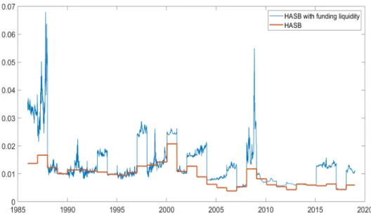
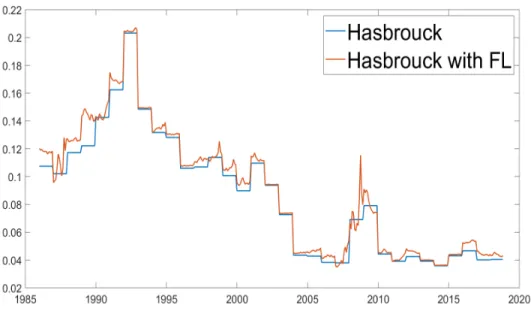
The averages we just discussed hide strong trends in historical transaction costs and marked spikes around crisis periods where trading frictions occur. In this section we will examine these dynamics for three anomalies that exhibited the largest difference in averages between the two extreme decile portfolios: size, realized volatility, and momentum.
a. Transaction costs and firm size
In Figures 1.3 and 1.4, we plot the transaction costs estimated with the Hasbrouck model (H-Model) at an annual frequency and the extended model with funding liquidity (FLH-Model), which shows the monthly movements associated with the TED spread, for a large firm (COCA COLA CO, with a market capitalization of 200 billions US dollars in 2018) and a small firm (ROCKY MOUNTAIN CHOCOLATE FACTORY, with a market capitalization of 22 millions US dollars in 2018). These two individual securities capture both the historical trends in transaction costs and the large fluctuations associated with trading frictions and captured by the TED spread. For both the large firm, COCA-COLA, and the small firm, ROCKY MOUNTAIN, we note a declining trend over time in transaction costs, from around 200 to 50 basis points for COCA-COLA and from about 750 to 100 basis points for ROCKY MOUNTAIN. This fact is known, but what is less documented is the huge spikes that occur when tight funding conditions impair trading. In the market crash of 1987 and the financial crisis of 2008, the transaction costs spiked at values between 500 and 650 basis points for COCA-COLA and between 1000 and 1500 basis points for ROCKY MOUNTAIN. The annual average estimates of the Hasbrouck[2009] model obscure these large fluctuations in trading costs.
Figure1.3 and Figure 1.4 here.
Figure 1.5 and Figure 1.6 feature the evolution over the 1986 to 2018 period of the transaction costs estimated monthly with both models for size portfolios (D1 for small firms and D10 for large firms). Figure 1.5 confirms the downward time trend for the average of small firms from 10% in 1986 to about 2% in 2018. Two large spikes appear. The 2008 financial crisis is of course one of the two but the largest one occurred in April 1992. In fact it is a culmination since it follows the recessionary period of 1990-1991 that brought the transaction cost to a level of 18% at the end of 1992 from a level of around 10% at the beginning of 1990. Monthly estimates from both models follow closely each other, with the liquidity estimate above the fixed cost of Hasbrouck[2009].
Figure1.5 and Figure 1.6 here.
In Figure 1.6 for large firms, a downward is also apparent between the beginning and the end of the sample, but during the decade 1990-2000 we observe a steady increase from
1992 to the beginning of 2000 for the liquidity model estimate of the transaction cost. It corresponds to an increase of 0.7 in the TED spread from the end of 1992 to the middle of year 2000. The peak at around 350 basis points for the liquidity model and 300 basis points for the H-Model occurred in the first months of the year 2000, coincident with the large jump in valuation during the tech bubble.
b. Transaction costs and volatility
Brunnermeier and Pedersen [2009] link market liquidity (that is the transaction price minus the fundamental value, in other words our measured transaction cost) to fundamental volatil-ity. The link is connected with margin constraints and is stronger when funding conditions are tight. High-volatility securities are more affected by intermediaries’ wealth shocks.
We measure these relations between the transaction costs of the individual stocks and their realized volatility. In Table 1.2, we report the average round-trip transaction costs for the realized-volatility decile portfolios. We observe that the high-volatility portfolio has a much higher transaction cost (around 9%) than the low-volatility portfolio (about 1%)12.
Funding liquidity adds another 40 points in average for the trading cost of high-volatility stocks. The Bayes factor selects the funding liquidity model in a higher proportion (around 80%) for lower-volatility deciles than for higher volatility stocks (about 65%).
Figure 1.7 and Figure 1.8 show the average transaction costs for high-volatility stocks and low-volatility stocks over time. We note the same declining trend in the transaction cost of the high-volatility stocks from about 10% in 1986 to 4% in 2018. However, as already noted for the small firms, we observe a large increase from the end of 1987 to 1994. The crash plus the recession of 1990-1991 and the jump in the funds rate in 1994 made high-volatility firms more expensive to trade (to more than 20%). The second peak appears of course during the 2008 financial crisis. For the low-volatility firms, the relative difference between the two models is more pronounced than for the high-volatility firms and varies between 20 and 50 basis points except for the crash of 1987 and the financial crisis of 2008, with spreads of 90 and 150 basis points respectively.
Figure1.7 and Figure 1.8 here.
12High-volatility stocks for a given year are the stocks that fall in the highest decile when we rank all stocks
c. Transaction Costs and Flight to Quality
Stocks of large firms and of low-volatility firms can be characterized as high-quality firms. In Brunnermeier and Pedersen [2009], flight to quality occurs when the market liquidity differential between high- and low-quality securities is larger bigger when speculator funding is tight. To rephrase this assertion, we can say that the flight to quality is the fact that the transaction cost differential between high- and low-quality securities (stocks of big and small firms or low-volatility and high-volatility stocks) is larger bigger when funding conditions are tight.
In the FLH-Model, the transaction cost for a firm i is obtained by cit = ci0,tp+ ci1,tp.F Lt.
To estimate the transaction cost of two stocks i and j for a given time period tp, we will
estimate the parameters ci
0,tp and ci1,tp for stock i and c j 0,tp and c j 1,tp for stock j. If ci1,tp > c j 1,tp,
the transaction cost differential between stock i and stock j will increase with the TED spread.
Table1.3presents the average value of parameters c1for size and realized volatility decile
portfolios. The values for c1 decrease with size and increase with volatility, supporting the
flight-to-quality condition. The other columns in Table 1.3 confirm that the transaction cost decreases with size and increases with volatility in absolute terms, but that it increases with size and decreases with volatility in percentage, which is consistent with what was apparent in the time-series evolution of the size and volatility portfolios.
Table 1.3 here.
d. Breaking down the transaction cost into its fixed and time-varying parts In Figure1.9, we separate the average transaction cost for all firms into its fixed part and its time-varying part. We plot the time series of the c0, which is fixed for a year, and of c1· F Lt
which varies with the level of the TED spread. We see again the downtrend in the fixed part and the time-varying that mimics a scaled version of the TED time series. When funding conditions are really tight, as during the 2008 crisis, the part of the transaction cost that depends on the funding liquidity can be more important than the other part.
1.4.3
Transaction Costs and other Financial Risk Measures
In this section, we summarize the main results associated with two risk measures that po-tentially affect the magnitude of the transaction cost. We estimate the time-varying part of the transaction cost ci
1· F Rt, where F Rt is in turn the VIX and theWeller [2019] measure of
tail risk. We report the average transaction costs for the anomalies that are most impacted by the financial risk, that is anomalies related to size and realized volatility, as well as their dynamics.
a. Transaction Costs and the VIX
The Chicago Board Option Exchanges (CBOE) Market Volatility Index, or VIX is a popular measure of the stock market’s expectation of volatility implied by S&P 500 index options. The VIX is often referred to as a “fear index” or the “fear gauge”(Whaley[2000]) for asset markets. A high value of the VIX is interpreted by investors as a potential sharp move of the market, either upward or downward, that is a higher expected volatility. Gromb and Vayanos [2002] and Brunnermeier and Pedersen[2009] predict that a higher market volatility tightens funding constraints of market makers and thereby reduces their liquidity-provision capacity. Nagel[2012] argues that when the VIX is high, market makers are financially constrained and therefore require a higher premium. More concretely, a higher market volatility makes stock prices move further away from their fundamental value, and therefore increase transaction costs.
Similarly to what we did for funding liquidity, we estimate the Hasbrouck model (H-Model) and the model with the VIX (VIXH-(H-Model). Our sample covers the period from January 1990 to June 2018. In Table 1.4, we report the average round-trip transaction cost for anomalies that produce the largest differences between the two extreme decile portfolios, that is the size of the firm (measured by SIZE, PRICE and NOA) and the realized volatility of the form (REALVOL). The spread between the trading costs of two extreme deciles for the three size-anomaly portfolios are wider than for funding liquidity. For SIZE, when we take in account the VIX in the Hasbrouck model, the transaction cost of the small-firm portfolio (D1) increases in average by 660 basis points while the big-firm one (D10) is 70 basis points larger. Overall, the spread between D1 and D10 for the VIXH-Model is 10%. For realized volatility, the trading-cost differential between D10 and D1 for the VIXH-Model more than doubled with respect to the FLH model (16.6% instead of 8%). The statistical support for
the VIXH-Model against the H model is again very strong for the larger-firm and the lower-volatility portfolios. The fact that VIX shocks include funding shocks and shocks from other sources may explain these larger spreads between extreme portfolios.
Table 1.4 and Figure 1.10 here.
Figure 1.10 show the dynamics of the transaction costs estimated from the two models (H-Model and VIXH-Model) for small and large firms and for high- and low-volatility portfo-lios. For the size-based anomaly portfolios, the patterns we uncovered with funding liquidity as a measure of financial risk remain the same both in terms of trend and large peaks, but the spreads between the H-Model and the VIXH-Model have widened considerably, as already indicated by the averages. For small firms, the differential in the beginning of the 90s is now close to 6%, while for large firms the peak around 2000 generates a spread o more than 2%. This increase in the trading-cost differential between the VIXH-Model and the H-Model is also present for the volatility portfolios. The VIX as a financial measure increases more the transaction costs of firms and produces relatively more peaks than funding liquidity. Flight to quality is also strongly supported when the VIX is used as the financial risk variable13.
b. Transaction Costs and Tail Risk
Market participants and regulators can rely on two prominent measures of high-frequency tail risk developed by Bollerslev and Todorov [2011] and Weller [2019]. The first paper uses high-frequency intra-daily data and short maturity out-of-the-money options on the S&P 500 index to construct an Investors Fears index. The second paper stresses the potential limitations imposed by the rarity of liquid, deep out-of-the-money options and proposes a new methodology that relies on the cross-section of bid-ask spreads. In terms of risk factors associated with extreme events, the second measure captures the aggregate economic shocks and the potential systemic threats underlying the cross-section of realized stock returns, while the first measure picks up the risk factors extracted from liquid options on the S&P 500 index.
In this section we estimate a model of transaction cost with tail risk (TRH-Model) using the measure proposed by Weller [2019]. Since it is an extreme risk factor extracted from high-frequency quote data for thousands of U.S. stocks, it seems particularly appropriate for
our analysis. The paper concentrates on the 2008 financial crisis and its aftermath so our trading-cost estimates will cover only the period from January 2008 to December 2014.
With respect to the relative importance of the VIX and tail risk to measure financial risk, Bollerslev et al. [2015] decompose the VIX into a jump tail risk component and normal-sized price fluctuations. They show that the compensation for jump tails risk makes up a larger part of the variance risk premium. Therefore, it will be interesting to measure the transaction cost associated with a tail risk measure. However, with the Weller[2019] measure, the scope of our analysis will be mainly focused on the 2008 financial crisis.
Table 1.1 and Table 1.5 here.
In Table1.1, the average transaction cost for the H-Model is estimated at 176 basis points and the addition of tail risk adds only 20 basis points to the trading cost. Table 1.5 features the trading costs for the size-related and volatility decile portfolios. The spread between the smallest-firm portfolio (D1) and the largest-firm portfolio (D1) for SIZE is 190 basis points for the H-Model and is increasing by 20 basis points for the TRH-Model. However, the Bayes factor shows strong evidence for the model with tail risk with 98% for the large firms and 72% for small firms. The volatility spread is larger with a trading cost of 50 basis points for the low-volatility portfolio (D1) and 500 basis points for the high-volatility portfolio, without the tail risk. Including the latter adds 40 basis points to the spread. Again the Bayes factor is very supportive of the model with tail risk. Interestingly, the lowest support occurs for the two extreme portfolios.
Figure 1.11 here.
After the 2008-2009 crisis, as shown in Figure1.11, the effective bid-ask spread subsided quickly for size and volatility. The patterns for both anomalies are similar to what was observed with the VIX in the later part of the sample. Finally, flight to quality is also supported with tail risk as the financial risk variable14.
1.5
After-trading-cost Performance of Anomalies
In this section we will evaluate the effect of accounting for transaction costs on the per-formance of so-called anomaly strategies, which consist in building long-short portfolios by