Every Choice Function is Backwards-Induction Rationalizable
∗Walter Bossert and Yves Sprumont Department of Economics and CIREQ
University of Montreal [email protected]
This version: January 31, 2013
Abstract. A choice function is backwards-induction rationalizable if there exists a finite perfect-information extensive-form game such that, for each subset of alternatives, the backwards-induction outcome of the restriction of the game to that subset of alterna-tives coincides with the choice from that subset. We prove that every choice function is backwards-induction rationalizable. Journal of Economic Literature Classification Num-bers: C72; D70.
∗ We thank Sean Horan for useful discussions. Financial support from the Fonds de
Recherche sur la Soci´et´e et la Culture of Qu´ebec and the Social Sciences and Humanities Research Council of Canada is gratefully acknowledged.
1
Introduction
This paper studies how the equilibrium outcome of a game varies with the set of feasible alternatives. We focus on finite perfect-information extensive-form games where all players have strict preferences over the alternatives attached to the terminal nodes. In any such game, Kuhn’s (1953) backwards-induction algorithm yields a unique outcome. If only a subset of alternatives remains feasible, pruning the original tree of all branches leading to infeasible alternatives defines a new game. Applying Kuhn’s algorithm to this restricted game again yields a unique outcome. Applying the algorithm to every restricted game thus generates a choice function, that is, a mapping selecting a single alternative from each feasible subset. We are interested in the general properties of this choice function, namely, those that do not depend on the number of players or the particular structure of the game tree.
It should be clear that such a choice function need not be well-behaved. Consider for instance the game G4 in Figure 1 where we indicate the relevant parts of the players’
pref-erences next to each decision node and the corresponding outcome next to each terminal node. The backwards-induction outcome of that game is alternative 3. The outcome of the game restricted to the feasible set {1, 2} is 1, the outcome restricted to {1, 3} is 1, and the outcome restricted to {2, 3} is 2. This is the choice function f4 in Table 1, omitting
the trivial choices from singletons. The collective choice behavior described by this choice function is highly irrational since the alternative chosen from the universal set is the only alternative that is never chosen from any pair—the Condorcet loser of the base relation associated with f4.
Up to a relabeling of the alternatives, Table 1 depicts all the possible three-alternative choice functions. The reader will easily check that each of the choice functions f1, f2, f3, f4
is generated by the game bearing the corresponding label in Figure 1. This shows that when there are only three conceivable alternatives, the backwards-induction outcome of a game may change in a totally arbitrary fashion with the set of feasible alternatives.
B f1(B) f2(B) f3(B) f4(B)
{1, 2} 1 1 1 1
{1, 3} 1 3 1 1
{2, 3} 2 2 2 2
{1, 2, 3} 1 1 2 3
. . . . . . . . . . . . . . . . . . . . . . . . . . . . . . . . . . . . . . . . . . . . . . . . . . . . . . . . . . . . . . . . . . . . . . . . . . . . . . . . . . . . . . . . . . . . . . . . . . . . . . . . . . . . . . . . . . . . . . . . . . . . . . . . . . . . . . . . . . . . . . . . . . . . . . . . . . . . . . . . . . . . . . . . . . . . . . . . . . . . . . . . . . . . . . . . . . . . . . . . . . ... ... ... ... ... ... ... ... ... ... ... ... ... ... ... ... ... ... ... ... ... ... ... ... ... ... ... ... ... ... ... ... ... • • • • 1 2 3 1 2 3
(a) The game G1.
. . . . . . . . . . . . . . . . . . . . . . . . . . . . . . . . . . . . . . . . . . . . . . . . . . . . . . . . . . . . . . . . . . . . . . . . . . . . . . . . . . . . . . . . . . . . . . . . . . . . . . . . . . . . . . . . . . . . . . . . . . . . . . . . . . . . . . . . . . . . . . . . . . . . . . . . . . . . . . . . . . . . . . . . . . . . . . . . . . . . . . . . . . . . . . . . . . . . . . . . . . . . . . . . . . . . . . . . . . . . . . . . . . . . . . . . . . . . . . . . . . . . . . . . . . . . . . . . . . . . . . . . . . . . . . . . . . . . . . . . . . . . . . . . . . . . . . . . . . . . . . ... ... ... ... ... ... ... . . . . . . . . . . . . . . . . . . . . . . . . . . . . . . . . . . . . . . . . . . . . . . . . . . . . . . . . . . . . . . . . . . . . . . . . . . . . . . . . . . . . . . . . . . . . . . . . . . . . . . . . . . . . . . . . . . . . . . . . . . . . . . . . . . . . . . . . . . . . . . . . . . ... ... ... ... ... ... ... • • • • • 3 1 2 2 3 1 2 3 (b) The game G2. . . . . . . . . . . . . . . . . . . . . . . . . . . . . . . . . . . . . . . . . . . . . . . . . . . . . . . . . . . . . . . . . . . . . . . . . . . . . . . . . . . . . . . . . . . . . . . . . . . . . . . . . . . . . . . . . . . . . . . . . . . . . . . . . ... .. .. .. .. .. .. .. .. .. .. .. .. .. .. .. .. .. .. .. .. .. .. .. .. .. .. .. .. .. .. .. .. .. .. .. .. .. .. .. .. .. .. .. .. .. .. .. .. .. .. .. .. .. .. .. .. .. .. .. .. .. .. .. .. .. .. .. .. .. .. .. .. .. .. .. .. .. .. .. ... ... ... ... ... ... ... ... ... ... ... ... ... ... ... ... ... ... ... ... ... ... ... ... ... ... ... ... ... ... ... ... ... ... ... ... ... ... .. .. .. .. .. .. .. .. .. .. .. .. .. .. .. .. .. .. .. .. .. .. .. .. .. .. .. .. .. .. .. .. .. .. .. .. .. .. .. .. .. .. .. .. .. .. .. .. .. .. .. .. .. .. .. .. .. .. .. .. .. .. .. .. .. .. .. .. .. .. .. .. .. .. .. ... ... ... ... ... ... ... ... ... ... ... ... ... ... ... ... ... ... ... ... ... ... ... ... ... ... ... ... ... ... ... ... ... • • • • • • • • • 1 2 3 3 1 2 2 1 3 1 2 3 1 2 3 (c) The game G3. . . . . . . . . . . . . . . . . . . . . . . . . . . . . . . . . . . . . . . . . . . . . . . . . . . . . . . . . . . . . . . . . . . . . . . . . . . . . . . . . . . . . . . . . . . . . . . . . . . . . . . . . . . . . . . . . . . . . . . . . . . . . . . . . . . . . . . . . . . . . . . . . . . . . . . . . . . . . . . . . . . . . . . . . . . . . . . . . . . . . . . . . . . . . . . . . . . . . . . . . . . . . . . . . . . . . . . . . . . . . . . . . . . . . . . . . . . . . . . . . . . . . . . . . . . . . . . . . . . . . . . . . . . . . . . . . . . . . . . . . . . . . . . . . . . . . . . . . . . . . . .. . . . . . . . . . . . . . . . . . . . . . . . . . . . . . . . . . . . . . . . . . . . . . . . . . . . . . . . . . . . . . . . . . . . . . . . . . . . . . . . . . . . . . . . . . . . . . . . . . . . . . . . . . . . . . . . . . . . . . . . . . . . . . . . . ... ... ... ... ... ... ... ... ... ... ... ... ... ... . . . . . . . . . . . . . . . . . . . . . . . . . . . . . . . . . . . . . . . . . . . . . . . . . . . . . . . . . . . . . . . . . . . . . . . . . . . . . . . . . . . . . . . . . . . . . . . . . . . . . . . . . . . . . . . . . . . . . . . . . . . . . . . . . . . . . . . . . . . . . . . . . .. . . . . . . . . . . . . . . . . . . . . . . . . . . . . . . . . . . . . . . . . . . . . . . . . . . . . . . . . . . . . . . . . . . . . . . . . . . . . . . . . . . . . . . . . . . . . . . . . . . . . . . . . . . . . . . . . . . . . . . . . . . . . . . . . ... ... ... ... ... ... ... ... ... ... ... ... ... ... . . . . . . . . . . . . . . . . . . . . . . . . . . . . . . . . . . . . . . . . . . . . . . . . . . . . . . . . . . . . . . . . . . . . . . . . . . . . . . . . . . . . . . . . . . . . . . . . . . . . . . . . . . . . . . . . . . . . . . . . . . . ... ... ... ... ... ... ... • • • • • • • • • • • 1 3 2 2 1 2 3 1 3 1 1 2 1 2 1 3 1 2 (b) The game G4.
Figure 1: The three-alternative case.
This result generalizes. Say that a choice function is backwards-induction rationalizable if there exists a finite perfect-information extensive-form game such that, for each subset of alternatives, the backwards-induction outcome of the restriction of the game to that subset of alternatives coincides with the choice from that subset. We prove that every choice function is backwards-induction rationalizable.
Our paper belongs to an emerging literature applying the revealed preference ap-proach to the study of collective decisions. The general goal is to identify the testable restrictions of the main theories of collective decision-making when individual preferences are not observable. We briefly review here the part of that literature which deals with noncooperative game-theoretic solution concepts.
correspon-dences defined over Cartesian subproducts of a given n-player normal game form. They identify necessary and sufficient conditions under which there exist n preferences over the conceivable joint actions such that the joint actions selected from each subgame form coincide with the Nash equilibria of the corresponding subgame. Lee (2012) characterizes choice behavior that is rationalizable via Nash equilibria of zero-sum games.
Ray and Zhou (2001) fix a finite-length game tree and an assignment of the decision nodes to a given set of n agents. They study choice functions defined over the restrictions of this game form. They give conditions under which there exist n (strict) preferences over the terminal nodes such that the alternative chosen in each restricted game form coincides with the backwards-induction outcome of the game generated by these preferences and the restricted game form. See also Ray and Snyder (2003).
In contrast with Ray and Zhou (2001) we do not fix the number of players or the grand game form. The choice functions we consider are therefore defined on subsets of alternatives—as in Arrow’s (1959) classical formulation—rather than on restricted game forms. We do this in order to identify the behavioral implications of backwards induction which do not depend on the particular characteristics of the environment. It turns out that there is none. Xu and Zhou (2007) perform the same exercise as ours under the rather particular restriction that each alternative can be attached to a terminal node of the grand game form once and only once. This restriction does constrain the choice functions that can be rationalized. While Xu and Zhou (2007) note (without a proof) that all three-alternative choice functions are backwards-induction rationalizable in the unrestricted-population case without their additional condition, they explicitly state that the general case represents an open question.
The unrestricted-population approach we follow in this paper is well established in economic theory. Our “anything-goes theorem” is in the spirit of results obtained in completely different contexts such as the Debreu (1974) – Mantel (1974) – Sonnenschein (1973) theorem on the aggregate excess demand of an exchange economy or McGarvey’s (1953) theorem on majority tournaments.
2
Definitions
Let A = {1, . . . , m} be a finite universal set of alternatives. For any non-empty subset B of A, the power set of B excluding the empty set is denoted by P(B). A choice function (on B) is a mapping f : P(B) → B such that f (C) ∈ C for all C ∈ P(B). An ordering is a reflexive, complete, transitive and antisymmetric relation. We denote by RB the set of
orderings on B.
A choice function f on B is best-element rationalizable if there exists an ordering R∗ on B such that
f (C) = max(C; R∗)
for all C ∈ P(B), where max(C; R∗) = {a ∈ C | aR∗b for all b ∈ C}. In this case, we say that R∗ is a best-element rationalization of f or that R∗ best-element rationalizes f . If there are at most two alternatives in B, any choice function f on B is best-element rationalizable: the case in which B is a singleton is trivial and if B contains exactly two elements, f is best-element rationalized by the relation R∗ given by f (B)R∗b where {b} = B \ {f (B)}.
The choice function f is (irrational) of degree k ≥ 1 if
(i) there exists an ordering R∗ on B and a collection C = {C1, . . . , Ck} of k distinct
subsets of B such that f (C) 6= max(C; R∗) for all C ∈ C and f (C) = max(C; R∗) for all C ∈ P(B) \ C; and
(ii) for all orderings R0 on B and for all collections C0 = {C10, . . . , Ck00} of k 0
< k distinct subsets of B, there exists C ∈ P(B) \ C0 such that f (C) 6= max(C; R0).
In this case, we say that R∗ underlies the choice function f and we call C the collection of critical sets of f with respect to R∗.
Let ≺ be a transitive and asymmetric relation on a non-empty and finite set N . We say that n ∈ N is a direct predecessor of n0 ∈ N if n ≺ n0 and there exists no n00 ∈ N such that n ≺ n00 ≺ n0. Equivalently, we say that n0 is a direct successor of n in this case. The set of direct predecessors of n ∈ N is denoted by P (n), and S(n) is the set of direct successors of n.
A tree Γ is given by a quadruple (0, D, T, ≺), where: (i) 0 is the root ;
(ii) D is a finite set of decision nodes such that 0 ∈ D;
(iii) T is a non-empty and finite set of terminal nodes such that D ∩ T = ∅;
(iv) ≺ is a transitive and asymmetric precedence relation on the set of all nodes N = D ∪ T such that:
(iv.a) P (0) = ∅ and |S(0)| ≥ 1;
(iv.b) for all n ∈ D \ {0}, |P (n)| = 1 and |S(n)| ≥ 1; (iv.c) for all n ∈ T , |P (n)| = 1 and S(n) = ∅.
When considering two trees Γ and Γ0, we identify the components in the obvious fashion, that is, Γ = (0, D, T, ≺) and Γ0 = (00, D0, T0, ≺0). Likewise, the sets of direct predecessors and direct successors of a node n ∈ N according to ≺ are P (n) and S(n), whereas these sets for n ∈ N0 according to ≺0 are denoted by P0(n) and S0(n). This should not create any ambiguity.
A path in Γ from a decision node n ∈ D to a terminal node n0 ∈ T (of length K ∈ N) is an ordered (K + 1)-tuple (n0, n1, . . . , nK) ∈ N|K+1| such that n = n0, {nk−1} = P (nk)
for all k ∈ {1, . . . , K} and nK = n0.
A game (on B) is a triple G = (Γ, g, R) where Γ is a tree, g: T → B is an outcome function that assigns an alternative g(n) ∈ B to each terminal node n ∈ T , and R: D → RB is a preference assignment map that assigns an ordering R(n) on B to each decision
node. This is a simplified version of a perfect-information game because the set of players is implicitly identified with the set of decision nodes and preferences are assumed to be antisymmetric. Again, we use the obvious notation (Γ0, g0, R0) for a game G0 etc.
Let G be a game on B. For any C ∈ P(B) such that C ⊆ g(T ), the restriction of G to C is the game G|C = G0 = (Γ0, g0, R0) on C given by:
(i) 00 = 0;
(ii) D0 = {n ∈ D | there exist n0 ∈ g−1(C) and a path in Γ from n to n0};
(iii) T0 = g−1(C);
(iv) ≺0 is the restriction of ≺ to N0 = D0∪ T0;
(v) g0 is the restriction of g to T0;
(vi) for all n ∈ D0, R0(n) is the restriction of R(n) to C.
See Figure 2 for an illustration of a game G on a set B = {1, 2, 3, 4, 5} and its restriction G0 = G|C to C = {1, 4}. The arrows emanating from the terminal nodes point to the respective outcomes according to the outcome functions of the games.
D . . . . . . . . . . . . . . . . . . . . . . . . . . . . . . . . . . . . . . . . . . . . . . . . . . . . . . . . . . . . . . . . . . . . . . . . . . . . . . . . . . . . . . . . . . . . . . . . . . . . . . . . . . . . . . . . . . . . . . . . . . . . . . . . ... .. .. .. .. .. .. .. .. .. .. .. .. .. .. .. .. .. .. .. .. .. .. .. .. .. .. .. .. .. .. .. .. .. .. .. .. .. .. .. .. .. .. .. .. .. .. .. .. .. .. .. .. .. .. .. .. .. .. .. .. .. .. .. .. .. .. .. .. .. .. .. .. .. .. .. .. .. .. .. ... ... ... ... ... .. .. .. .. .. .. .. .. .. .. .. .. .. .. .. .. .. .. .. .. .. .. .. .. .. .. .. .. .. .. .. .. .. .. .. .. .. ... ... ... ... ... ... ... ... ... ... ... ... ... ... ... ... ... ... .. .. .. .. .. .. .. .. .. .. .. .. .. .. .. .. .. .. .. .. .. .. .. .. .. .. .. .. .. .. .. .. .. .. .. .. .. .. .. ... .. .. .. .. .. .. .. .. .. .. .. .. .. .. .. .. .. .. .. .. .. .. .. .. .. .. .. .. .. .. .. .. .. .. .. .. .. .. .. . ... ... ... ... ... ↑ ↑ ↑ ↑ ↑ ↑ g(T ) 1 2 3 4 1 5 T • • • • • • • • • • • D0 . . . . . . . . . . . . . . . . . . . . . . . . . . . . . . . . . . . . . . . . . . . . . . . . . . . . . . . . . . . . . . . . . . . . . . . . . . . . . . . . . . . . . . . . . . . . . . . . . . . . . . . . . . . . . . . . . . . . . . . . . . . . . . . . ... .. .. .. .. .. .. .. .. .. .. .. .. .. .. .. .. .. .. .. .. .. .. .. .. .. .. .. .. .. .. .. .. .. .. .. .. .. .. .. .. .. .. .. .. .. .. .. .. .. .. .. .. .. .. .. .. .. .. .. .. .. .. .. .. .. .. .. .. .. .. .. .. .. .. .. .. .. .. .. ... ... ... ... ... .. .. .. .. .. .. .. .. .. .. .. .. .. .. .. .. .. .. .. .. .. .. .. .. .. .. .. .. .. .. .. .. .. .. ... .. .. .. .. .. .. .. .. .. .. .. .. .. .. .. .. .. .. .. .. .. .. .. .. .. .. .. .. .. .. .. .. .. .. .. .. .. .. .. . ... ... ... ... ... ↑ ↑ ↑ g(T0) 1 4 1 T0 • • • • • • •
Figure 2: A game on B = {1, 2, 3, 4, 5} and its restriction to C = {1, 4}.
For each decision node n ∈ D, we denote by en(G) the backwards-induction outcome
of the subgame of G rooted at n. This outcome is defined in the usual way: we first set en(G) = g(n) for all n ∈ T , then define recursively en(G) = max({en0(G) | n0 ∈ S(n)} ; R(n))
for all n ∈ D. To simplify notation we write e0(G) = e(G). Because G is a finite
perfect-information game and all preferences are antisymmetric, the backwards-induction outcome of any subgame of G (including G itself) exists and is unique. For every C ∈ P(B), the backwards-induction outcome of G|C is also well defined.
A choice function f on B is backwards-induction rationalizable if there exists a game G = (Γ, g, R) on B such that f (C) = e(G|C) for all C ∈ P(B). In this case, we say that G is a backwards-induction rationalization of f or that G backwards-induction rationalizes f .
3
Results
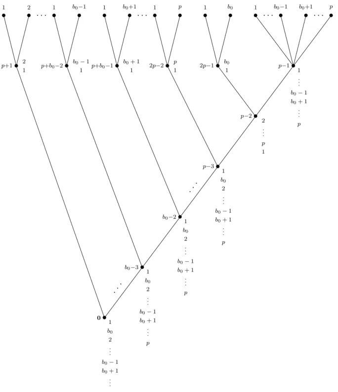
The following two lemmas provide important steps in the proof of our main result. We begin with choice functions of degree 1 whose only critical set is the set of all alternatives. Lemma 1 Let B ∈ P(A), let R∗ ∈ RB and let b0 ∈ B \ max(B; R∗). The choice function
f on B defined by f (C) = ( max(C; R∗) if C 6= B, b0 if C = B is backwards-induction rationalizable.
Proof. Let B, R∗, b0 and f be as in the statement of the lemma. Without loss of
on {1, . . . , p}. Thus, the best element in a non-empty subset C of B according to R∗ can be written as min(C) without any danger of ambiguity. Moreover, b0 6= 1. Let G be the
game on B depicted in Figure 3. For simplicity of presentation, we do not include the labels of the terminal nodes but, instead, attach the outcomes according to the outcome function. The preferences assigned to each decision node (that is, to each player) are displayed to the right of the respective node. We simplify our exposition by restriction attention to the part of the preferences that is relevant for the argument. For instance, all that we need to know regarding the preferences associated with nodes p + 1, . . . , 2p − 1 is that one of the two alternatives that can feature as a possible choice at the respective node is preferred to the other. Analogously, there is no need to specify where the alternative b0 is ranked in the preference assigned to node p − 1 because it can never appear as a
.. .. .. .. .. .. .. .. .. .. .. .. .. .. .. .. .. .. .. .. .. .. .. .. .. .. .. .. .. .. .. .. .. .. .. .. .. .. .. .. .. .. .. .. .. .. .. .. .. .. .. .. .. .. .. .. .. .. .. .. .. .. .. .. .. .. .. .. .. .. .. .. .. .. .. .. .. .. .. .. .. .. .. .. .. .. .. .. .. .. .. .. .. .. .. .. .. .. .. .. .. .. .. .. .. .. .. .. .. .. .. .. .. .. .. .. .. .. .. .. .. .. .. .. .. .. .. .. .. .. .. .. .. .. .. .. .. .. .. .. .. .. .. .. .. .. .. .. .. .. .. .. .. .. .. .. .. .. .. .. .. .. .. .. .. .. .. .. .. .. .. .. .. .. .. .. .. .. .. .. .. .. .. .. .. .. .. .. .. .. .. .. .. .. .. .. .. .. .. .. .. .. .. .. .. .. .. .. .. .. .. .. .. .. .. .. .. .. .. .. .. .. .. .. .. .. .. .. .. .. .. .. .. .. .. .. .. .. .. .. .. .. .. .. .. .. .. .. .. .. .. .. .. .. .. .. .. .. .. .. .. .. .. .. .. .. .. .. .. .. .. .. .. .. .. .. .. .. .. .. .. .. .. .. .. .. .. .. .. .. .. .. .. .. .. .. .. .. .. .. .. .. .. .. .. .. .. .. .. .. .. .. .. .. .. .. .. .. .. .. .. .. .. .. .. .. .. .. .. .. .. .. .. .. .. .. .. .. .. .. .. .. .. .. .. .. .. .. .. .. .. .. .. .. .. .. .. .. .. .. .. .. .. .. .. .. .. .. .. .. .. .. .. .. .. .. .. .. .. .. .. .. .. .. .. .. .. .. .. .. .. .. .. .. .. .. .. .. .. .. .. .. .. .. .. .. .. .. .. .. .. .. .. .. .. .. .. .. .. .. .. .. .. .. .. .. .. .. .. .. .. .. .. .. .. .. .. .. .. .. .. .. .. .. .. .. .. .. .. .. .. .. .... ... ... ... ... ... ... ... ... ... ... ... ... ... ... ... ... ... ... ... ... ... ... ... ... ... ... ... ... ... ... ... ... ... ... ... ... ... ... ... ... ... ... ... ... ... ... ... ... ... ... ... ... ... ... ... ... ... .. ... ... ... ... ... ... ... ... ... ... ... .. ... ... ... ... ... ... ... ... ... ... ... ... ... ... ... ... ... ... ... ... ... ... ... ... ... ... ... ... ... ... ... ... ... ... ... ... ... ... ... ... ... ... ... ... ... ... ... ... ... ... ... . . . . . . . . . . . . . . . . . . . . . . . . . . . . . . . . . . . . . . . . . . . . . . . . . . . . . . . . . . . . . . . . . . . . . . . . . . . . . . . . . . . . . . . . . . . . . . . . . . . . . . . . . . . . . . . . . . . . . . . . . . . . . . . . . . . . . . . . . . . . . . . . . . . . . . . . . . . . . . . . . . . . . . . . . . . . . . . . . . . . . . . . . . . . . . . . . . . . . . . . . . . . . . . . . . . . . ... ... ... ... ... ... ... ... ... ... ... ... ... ... ... ... ... ... ... ... ... ... ... ... ... ... ... ... ... ... ... ... ... ... ... ... ... ... ... ... ... ... ... ... ... ... ... ... ... ... ... ... ... ... ... ... ... ... .. ... ... ... ... ... ... ... ... ... ... ... ... ... ... ... ... ... ... ... ... ... .... .. .. .. .. .. .. .. .. .. .. .. .. .. .. .. .. .. .. .. .. .. .. .. .. .. .. .. .. .. .. .. .. .. .. .. .. .. .. .. .. .. .. .. .. .. .. .. .. .. .. .. .. .. .. .. .. .. .. .. .. .. .. .. .. .. .. .. .. .. .. .. .. .. .. .. .. .. .. .. .. .. .. .. .. .. .. .. .. .. .. .. .. .. .. .. .. .. .. .. .. .. .. .. .. .. .. .. .. .. .. .. .. .. .. .. .. .. .. .. .. .. .. .. .. .. .. .. .. .. .. .. .. .. .. .. .. .. .. .. .. .. .. .. .. .. .. .. .. .. .. .. .. .. .. .. .. .. .. .. .. .. .. .. .. .. .. .. .. .. .. .. .. .. .. .. .. .. .. .. .. .. .. .. .. .. .. .. .. .. .. .. .. .. .. .. .. .. .. .. .. .. .. .. .. .. .. .. .. .. .. .. .. .. .. .. .. .. .. .. .. .. .. .. .. .. .. .. .. .. .. .. .. .. .. .. .. .. .. .. .. .. .. .. .. .. .. .. .. .. .. .. .. .. .. .. .. .. .. .. .. .. .. .. .. .. .. .. .. .. .. .. .. .. .. .. .. .. .. .. .. .. .. .. .. .. .. .. .. .. .. .. .. .. .. .. .. .. .. .. .. .. .. .. .. .. .. .. .. .. .. .. .. .. .. .. .. .. .. .. .. .. .. .. .. .. .. .. .. .. .. .. .. .. .. .. .. .. .. .. .. .. .. .. .. .. .. .. .. .. .. .. .. .. .. .. .. .. .. .. .. .. .. .. .. ... ... ... ... ... ... ... ... ... ... ... ... ... ... ... ... ... ... ... ... ... ... ... ... ... ... ... ... ... ... ... ... ... ... ... ... ... ... ... ... ... ... ... ... ... ... ... ... ... ... ... ... ... ... ... ... ... ... ... . ... ... ... ... ... ... ... ... ... ... ... .. .. .. .. .. .. .. .. .. .. .. .. .. .. .. .. .. .. .. .. .. .. .. .. .. .. .. .. .. .. .. .. .. .. .. .. .. .. .. .. .. .. .. .. .. .. .. .. .. .. .. .. .. .. .. .. .. .. .. .. .. .. .. .. .. .. .. .. .. .. .. .. .. .. .. .. .. .. .. .. .. .. .. .. .. .. .. .. .. .. .. .. .. .. .. .. .. .. .. .. .. .. .. .. .. .. .. .. .. .. .. .. .. .. .. .. .. .. .. .. .. .. .. .. .. .. .. .. .. .. .. .. .. .. .. .. .. .. .. .. .. .. .. .. .. .. .. .. .. .. .. .. .. .. .. .. .. .. .. .. .. .. .. .. .. .. .. .. .. .. .. .. .. .. .. .. .. .. .. .. .. .. .. .. .. .. .. .. .. .. .. .. .. .. .. .. .. .. .. .. .. .. .. .. .. .. .. .. .. .. .. .. .. .. .. .. .. .. .. .. .. .. .. .. .. .. .. .. .. .. .. .. .. .. .. .. .. .. .. .. .. .. .. .. .. .. .. .. .. .. .. .. .. .. .. .. .. .. .. .. .. .. .. .. .. .. .. .. .. .. .. .. .. .. .. .. .. .. .... ... ... ... ... ... ... ... ... ... ... ... ... ... ... ... ... ... ... ... ... ... ... ... ... ... ... ... ... ... ... ... ... ... ... ... ... ... ... ... ... ... ... ... ... ... ... ... ... ... ... ... ... ... ... ... ... ... .. ... ... ... ... ... ... ... ... ... ... ... .. .. .. .. .. .. .. .. .. .. .. .. .. .. .. .. .. .. .. .. .. .. .. .. .. .. .. .. .. .. .. .. .. .. .. .. .. .. .. .. .. .. .. .. .. .. .. .. .. .. .. .. .. .. .. .. .. .. .. .. .. .. .. .. .. .. .. .. .. .. .. .. .. .. .. .. .. .. .. .. .. .. .. .. .. .. .. .. .. .. .. .. .. .. .. .. .. .. .. .. .. .. .. .. .. .. .. .. .. .. .. .. .. .. .. .. .. .. .. .. .. .. .. .. .. .. .. .. .. .. .. .. .. .. .. .. .. .. .. .. .. .. .. .. .. .. .. .. .. .. .. .. .. .. .. .. .. .. .. .. .. .. .. .. .. .. .. .. .. .. .. .. .. .. .. .. .. .. .. .. .. .. .. .. .. .. .. .. .. .. .. ... ... ... ... ... ... ... ... ... ... ... ... ... ... ... ... ... ... ... ... ... ... ... ... ... ... ... ... ... ... ... ... ... ... ... ... ... ... ... ... ... ... ... ... ... ... ... ... ... ... ... ... ... ... ... ... ... ... ... . ... ... ... ... ... ... ... ... ... ... ... .. . . . . . . . . . . . . . . . . . . . . . . . . . . . . . . . . . . . . . . . . . . . . . . . . . . . . . . . . . . . . . . . . . . . . . . . . . . . . . . . . . . . . . . . . . . . . . . . . . . . . . . . . . . . . . . . . . . . . . . . . . . . . . . . . . . . . . . . . . . . . . . . . . . . . . . . . . . . . . . . . . . . . . . . . . . . . . . . . . . . . . . . . . . . . . . . . . . . . . . . . . . . . . . . . . . . . . .... ... ... ... ... ... ... ... ... ... ... ... ... ... ... ... ... ... ... ... ... ... ... ... ... ... ... ... ... ... ... ... ... ... ... ... ... ... ... ... ... ... ... ... ... ... ... ... ... ... ... ... ... ... ... ... ... ... .. ... ... ... ... ... ... ... ... ... ... ... .. · · · · ··· ··· • • • • • • • • • • • • • • • • • • • • • • • • • 1 2 1 b0−1 1 b0+1 1 p 1 b0 1 b0−1 b0+1 p 1 b0 2 . . . b0− 1 b0+ 1 . . . p 0 1 b0 2 . . . b0− 1 b0+ 1 . . . p b0−3 1 b0 2 . . . b0− 1 b0+ 1 . . . p b0−2 1 b0 2 . . . b0− 1 b0+ 1 . . . p p−3 2 . . . p 1 p−2 1 . . . b0− 1 b0+ 1 . . . p p−1 2 1 p+1 b0− 1 1 p+b0−2 b0+ 1 1 p+b0−1 p 1 2p−2 b0 1 2p−1
Figure 3: The game G on B in the proof of Lemma 1.
We claim that f (C) = e(G|C) for all C ∈ P(B). Let C ∈ P(B). We distinguish four cases.
Case 1. C = B. By definition of R(p − 1) and R(2p − 1), we have ep−1(G|B) =
ep−1(G|C) = 1 and e2p−1(G|C) = b0, hence
ep−2(G|C) = b0.
Since ep+q(G|C) 6= 1 for all q ∈ {1, . . . , p − 2}, we obtain from the definition of the
orderings R(p − 3), . . . , R(0) that
ep−2(G|C) = b0 ⇒ ep−3(G|C) = b0 ⇒ . . . ⇒ e0(G|C) = e(G|C) = b0 = f (C).
Case 2. C 6= B and min(C) = 1. Since C 6= B, there exists q ∈ {1, . . . , p − 1} such that ep+q(G|C) = 1. This in turn implies that
eq−1(G|C) = 1. (1)
Indeed, if q = p − 1, then ep+q(G|C) = 1 implies e2p−1(G|C) = 1. Since ep−1(G|C) = 1,
it follows that ep−2(G|C) = 1, establishing (1). On the other hand, if q < p − 1, then (1)
follows from the fact that ep+q(G|C) = 1 and max(C; R(q − 1)) = 1.
From (1) and the definition of the orderings R(q − 2), . . . , R(0), we obtain eq−1(G|C) = 1 ⇒ eq−2(G|C) = 1 ⇒ . . . ⇒ e0(G|C) = e(G|C) = 1 = f (C).
Case 3. C 6= B and min(C) = b0. Recall that b0 6= 1. Therefore 1 6∈ C and we obtain
ep−2(G|C) = b0 ⇒ ep−3(G|C) = b0 ⇒ . . . ⇒ e0(G|C) = e(G|C) = b0 = min(C) = f (C).
Case 4. C 6= B and min(C) 6∈ {1, b0}. In this case again, 1 6∈ C.
Case 4.1. b0 6∈ C. Since 1 6∈ C and b0 6∈ C, there exists q ∈ {1, . . . , p − 2} such that
ep+q(G|C) = min(C). By definition of R(q − 1), . . . , R(0),
ep+q(G|C) = min(C) ⇒ eq−1(G|C) = min(C) ⇒ . . . ⇒ e0(G|C) = e(G|C) = min(C) = f (C).
Case 4.2. b0 ∈ C and min(C) < b0. Then ep−1(G|C) = min(C) 6∈ {1, b0}, hence
ep−2(G|C) = min(C). By definition of R(p − 3), . . . , R(0) and because ep+q(G | C) /∈
{1, b0} for q ∈ {1, . . . , p − 2}, we obtain
ep−2(G|C) = min(C) ⇒ . . . ⇒ e0(G|C) = min(C) = f (C),
which completes the proof.
Lemma 2 Every choice function of degree 1 is backwards-induction rationalizable. Proof. Suppose f is a choice function of degree 1 on A = {1, . . . , m}. Without loss of generality, we assume that the underlying ordering R∗ is the natural ordering ≤ on A. As in the proof of Lemma 1, the best element in a non-empty subset B of A according to R∗ can thus be written as min(B). Let B0 be the unique critical set of f with respect to ≤.
Thus, f (B0) > min(B0) and f (B) = min(B) for all B ∈ P(A) \ {B0}. If B0 = A, then f
is backwards-induction rationalizable by Lemma 1. From now on, assume B0 6= A.
Consider the restriction of f to P(B0). By Lemma 1, there exists a game G0 on B0
that backwards-induction rationalizes this restriction. In particular, this implies that
e(G0|B0) = f (B0). (2)
Now define a game G on A as depicted in Figure 4. The root of the tree is 0. The set of decision nodes D is given by the union of {0, 1, 2} and the set of decision nodes D0 of
G0. Label all decision nodes of G0 so that no ambiguities can arise. The set of terminal
nodes T is the union of the set of terminal nodes T0 of G0 and 2 + |A \ B0| additional
distinct nodes. We only depict the outcomes assigned to these terminal nodes but not the labels attached to them.
Define ≺ on D ∪ T as follows: 0 is the direct predecessor of 1 and of one of the additional terminal nodes, 1 is the direct predecessor of 2 and of another of the new terminal nodes, 2 is the direct predecessor of the remaining |A \ B0| new nodes and of the
root of the tree G0, and the restriction of ≺ to D0 coincides with ≺0.
Let g be such that g(n) = g0(n) for all terminal nodes n ∈ T0 and as displayed in the
figure for all other nodes. Note that g assigns a different alternative in A \ B0 to each
node in the subset labeled A \ B0.
The preference assignment R is such that R(0) = R∗, R(1) has f (B0) as its best
element, followed by the remaining alternatives in A in their natural order, and R(2) first ranks the alternatives in A other than f (B0) in their natural order and has f (B0) as its
worst element. Each ordering R(n) corresponding to a decision node n of G0 is such that
. . . . . . . . . . . . . . . . . . . . . . . . . . . . . . . . . . . . . . . . . . . . . . . . . . . . . . . . . . . . . . . . . . . . . . . . . . . . . . . . . . . . . . . . . . . . . . . . . . . . . . . . . . . . . . . . . . . . . . . . . . . . . . . . . . . . . . . . . . . . . . . . . . . . . . . . . . . . . . . . . . . . . . . . . . . . . . . . . . . . . . . . . . . . . . . . . . . . . . . . . . . . . . . . . . . . . . . . . . . . . . . . . . . . . . . . . . . . . . . . . . . . . . . . . . . . . . . . . . . . . . . . . . . . . . . . . . . . . . . . . . . . . . . . . . . . . . . . . . . . . . . . . . . . . . . . . . . . . . . . . . . . . . . . . . . . . . . . . . . . . . . . . . . . . . . . . . . . . . . . . . . . . . . . . . . . . . . . . . . . . . . . . . . . . . . . . . . . . . . . . . . . . . . . . . . . . . . . . . . . . . . . . . . . . . . . . . . . . . . . . . . . . . . . . . . . . . . . . . . . . . . . . . . . . . . . . . . . . . . . . . . . . . . . . . . . . . . . . . . . . . . . . . . . . . . . . . . . . . . . . . . . . . . . . . . . . . . . . . . . . . . . . . . . . . . . . . . . . . . . . . . . . . . . . . . . . . . . . . . . . . . . . . . . . . . . . . . . . . . . . . . . . . . . . . . . . . . . . . . . . . . . . . . . . . . . . . . . . . . . . . . . . . . . . . . . . . . . . . . . . . . . . . . . . . . . . . . . . . . . . . . . . ... ... ... ... ... ... ... ... ... ... ... ... ... ... ... ... ... ... ... ... ... ... ... ... ... ... ... ... ... . . . . . . . . . . . . . . . . . . . . . . . . . . . . . . . . . . . . . . . . . . . . . . . . . . . . . . . . . . . . . . . . . . . . . . . . . . . . . . . . . . . . . . . . . . . . . . . . . . . . . . . . . . . . . . . . . . . . . . . . . . . . . . . . . . . . . . . . . . . . . . . . . . . . . . . . . . . . . . . . . . . . . . . . . . . . . . . . . . . . . . . . . . . . . . . . . . . . . . . . . . . . . . . . . . . . . . . . . . . . . . . . . . . . . . . . . . . . . . . . . . . . . . . . . . . . . . . . . . . . . . . . . . . . . . . . . . . . . . . . . . . . . . . . . . . . . . . . . . . . . . . . . . . . . . . . . . . . . . . . . . . . . . . . . . . . . . . . . . . . . . . . . . . . . . . . . . . . . . . . . . . . . . . . . . . . . . . . . . . . . . . . . . . . . . . . . . . . . . . . . . . . . . . . . . . . . . . . . . . . . . . . . . . . . . . . . . . . . . . . . . . . . . . . . . . . . . . . . . . . . . . . . . . . . . . . . . . . . . . . . . . . . . . . . . . . . . . . . . . . . . . . . . . . . . . . . . . . . . . . . . . . . . . . . . . . . . . . . . . . . . . . . . . . . . . . . . . . . . . . . . . . . . . . . . . . . . . . . . . . . . . . . . . . . . . . . . . . . . . . . . . . . . . . . . . . . . . . . . . . . . . . . . . . . . . . . . . . . . . . . . . . . . . . . . . . . . . . . . . . . . . . . . . . . . . . . . . . . . . . . . . . . . . . . . . . . . . . . . . . . . . . . . . . . . . . . . . . . . . . . . . . . . . . . . . . . . . . . . . . . . . . . . . . . . . . . . . . . . . . . . . . . . . . . . . . . . . . . . . . . . . . . . . . . . . . . . . . . . . . . . . . . . . . . . . . . . . . . . . . . . . . . . . . . . . . . . . . . . . . . . . . . . . . . . . . . . . . . ... ... ... ... ... ... ... ... ... ... ... ... ... ... ... ... ... ... ... ... ... ... ... ... ... ... ... ... ... ... ... ... ... ... ... ... ... ... ... ... .. ... ... ... ... ... ... ... ... ... ... ... ... .. · · · f (B0) min(B0) A \ B0 • • • • • • • • G0 1 . . . m 0 f (B0) 1 . . . f (B0) − 1 f (B0) + 1 . . . m 1 1 . . . f (B0) − 1 f (B0) + 1 . . . m f (B0) 2
Figure 4: The game G on A in the proof of Lemma 2.
We now show that G is a backwards-induction rationalization of f . Let B ∈ P(A). To show that e(G|B) = f (B), we distinguish three cases.
Case 1. min(B) < min(B0). This implies that min(B) 6∈ B0 and, thus, min(B) ∈ A \ B0.
Because min(B) < min(B0) < f (B0), we have min(B) 6= f (B0), hence min(B)R(2)b
for all b ∈ B. It follows that e2(G|B) = min(B). Thus, e1(G|B) = min(B) because
min(B)R(1) min(B0). Finally, we obtain e(G|B) = e0(G|B) = min(B) because min(B)
R(0)f (B0).
Case 2. min(B) = min(B0). We consider two subcases.
Case 2.1. B = B0. Thus, e(G0|B0) = f (B0) by (2). Because f (B0) 6∈ A \ B0, it follows
that e2(G|B0) = f (B0). By definition of R(1), f (B0)R(1) min(B0) and, thus, e1(G|B0) =
f (B0). Thus, by definition of the tree G, we obtain e(G|B) = e(G|B0) = f (B0) = f (B).
Case 2.2. B 6= B0. Two further subcases are distinguished.
Case 2.2.1. B ∩ B0 = B0. In this case, e(G0|(B ∩ B0)) = e(G0|B0) = f (B0). Since
B ∩ (A \ B0) 6= ∅ and f (B0) is the worst element according to R(2), we obtain e2(G|B) ∈
definition of R(1) that e1(G|B) = min(B0). Because min(B0) < f (B0) and R(0) is equal
to ≤, we obtain e(G|B) = min(B0) = min(B).
Case 2.2.2. B ∩ B0 6= B0. Since G0 backwards-induction rationalizes the restriction of
f to P(B0),
e(G0|(B ∩ B0)) = min(B ∩ B0) = min(B) = min(B0)
because both B and B0 must contain min(B) = min(B0). Since min(B) = min(B0) 6=
f (B0), we have min(B)R(2)b for all b ∈ B ∩ (A \ B0). Therefore e2(G | B) = min(B).
Next, e(G|B) = min(B) because min(B) = min(B0)R(0)f (B0).
Case 3. min(B0) < min(B). In this case min(B0) 6∈ B and hence B ∩ B0 6= B0. This
implies
e(G0|(B ∩ B0)) = min(B ∩ B0).
Again, we consider two subcases.
Case 3.1. min(B) = f (B0). Then we obtain e(G|B) = f (B0) = min(B) immediately
from the definition of R(0).
Case 3.2. min(B) 6= f (B0). Two further subcases can be distinguished.
Case 3.2.1. min(B) ∈ B0. In this case, e(G0|(B∩B0)) = min(B∩B0) = min(B) 6= f (B0).
By definition of R(2),
e2(G|B) = min{min(B ∩ (A \ B0)), e(G0|(B ∩ B0))}
= min{min(B ∩ (A \ B0)), min(B ∩ B0)}
= min(B). Because min(B0) 6∈ B, it follows that
e1(G|B) = min(B). (3)
Since min(B) 6= f (B0), either min(B) < f (B0) or min(B) > f (B0). In the first case, (3)
and the definition of R(0) imply that e(G|B) = min(B). In the second case, f (B0) /∈ B
and (3) therefore implies e(G|B) = min(B) by definition of the game G.
Case 3.2.2. min(B) ∈ A \ B0. Now min(B ∩ (A \ B0)) = min(B) 6= f (B0). If e(G0|(B ∩
B0)) 6= f (B0), the definition of R(2) implies
e2(G|B) = min{min(B ∩ (A \ B0)), e(G0|(B ∩ B0))}
= min{min(B), e(G0|(B ∩ B0))}
If e(G0|(B ∩ B0)) = f (B0), the definition of R(2) implies
e2(G|B) = min(B ∩ (A \ B0)) = min(B).
In both cases e2(G|B) = min(B). Since min(B0) 6∈ B, it follows that e1(G|B) = min(B).
The conclusion that e(G|B) = min(B) now follows by the same argument as in case 3.2.1.
Using the result of the above lemma, our theorem establishes that all choice functions are backwards-induction rationalizable.
Theorem 1 Every choice function is backwards-induction rationalizable.
Proof. Every best-element rationalizable choice function is trivially backwards-induction rationalizable and Lemma 2 shows that every choice function of degree 1 is backwards-induction rationalizable. We prove the theorem by backwards-induction on the degree of irrationality of a choice function. Let k > 1 and, as our induction hypothesis, suppose that every choice function of irrationality degree 1, . . . , k−1 is backwards-induction rationalizable. Consider a choice function f on A = {1, . . . , m}. Suppose that f is of degree k and let the ordering R∗ underlie f . Without loss of generality, let R∗ be the natural ordering ≤ on A. Let C = {C1, . . . , Ck} be the collection of critical sets of f with respect to R∗. Thus, by
definition, f (C) 6= min(C) for all C ∈ C and f (C) = min(C) for all C ∈ P(A) \ C. Pick C1, C2 ∈ C. We have
f (C1) 6= min(C1) and f (C2) 6= min(C2). (4)
For i ∈ {1, 2}, define the choice function fi(C) =
(
min(Ci) if C = Ci,
f (C) if C ∈ P(A) \ {Ci}.
By construction, each fi is of irrationality degree less than k and, by the induction
hy-pothesis, fi is backwards-induction rationalizable by a game Gi.
Let R0 be an ordering on A such that f (Ci)R0min(Ci) for i ∈ {1, 2}. Observe that
such an ordering exists if and only if
f (C1) 6= min(C2) or f (C2) 6= min(C1). (5)
To see that (5) is implied by (4), suppose that, by way of contradiction, f (C1) = min(C2) and f (C2) = min(C1).
Since f (Ci) ∈ Ci for i ∈ {1, 2}, we must have f (C1) ≤ f (C2) and f (C2) ≤ f (C1), hence
f (C1) = f (C2) because ≤ is antisymmetric. But then we obtain
f (C1) = f (C2) = min(C1) = min(C2),
contradicting (4).
Now construct a game G on A by letting the root 0 be such that it is associated with the ordering R(0) = R0 and has two direct successors, namely, the roots of G1 and G2,
and all other characteristics of the game G are inherited from G1 and G2 in the obvious
fashion. See Figure 5.
. . . . . . . . . . . . . . . . . . . . . . . . . . . . . . . . . . . . . . . . . . . . . . . . . . . . . . . . . . . . . . . . . . . . . . . . . . . . . . . . . . . . . . . . . . . . . . . . . . . . . . . . . . . . . . . . . . . . . . . . . . . . . . . . . . . . . . . . . . . . . . . . . . . . . . . . . . . . . . . . . . . . . . . . . . . . . . . . . . . . . . . . . . . . . . . . . . . . . . . . . . . . . . . . . . . . . . . . . . . . . . . . . . . . . . . . . . . . . . . . . . . . . . . . . . . . . . . . . . . . . . . . . . . . . . . . . . . . . . . . . . . . . . . . . . . . . . . . . . . . . . . . . . . . . . . . . . . . . . . . . . . . . . . . . . . . . . . . . . . . . . . . . . . . . . . . . . . . . . . . . . . . . . . . . . . . . . . . . . . . . . . . . . . . . . . . . . . . . . . . . . . ... ... ... ... ... ... ... ... ... ... ... ... ... ... ... ... ... • •... • .. .. .. .. .. .. .. .. .. .. .. .. .. .. .. .. .. .. .. .. .. .. .. .. .. .. .. .. .. .. .. .. .. .. .. .. .. .. .. .. .. .. .. .. .. .. .. .. .. .. .. .. .. .. .. .. .. .. .. .. .. .. .. .. .. .. .. .. .. .. .. .. .. ...... ... ... ... ... ... ... ... ... ... ... ... ... .. G1 .. .. .. .. .. .. .. .. .. .. .. .. .. .. .. .. .. .. .. .. .. .. .. .. .. .. .. .. .. .. .. .. .. .. .. .. .. .. .. .. .. .. .. .. .. .. .. .. .. .. .. .. .. .. .. .. .. .. .. .. .. .. .. .. .. .. .. .. .. .. .. .. .. .. .. .. .. .. .. ...... ... ... ... ... ... ... ... ... ... ... ... ... .. G2 0 R0
Figure 5: The game G on A in the proof of Theorem 1.
By construction, we have
e(G|C) = max({e(G1|C), e(G2|C)}; R0)
for all C ∈ P(A).
If C 6∈ {C1, C2}, it follows that e(G1|C) = e(G2|C) = f (C) and hence e(G|C) = f (C).
If C = C1, we obtain e(G|C) = e(G|C1) = max({e(G1|C1), e(G2|C1)}; R0) = max({f1(C1), f2(C1)}; R0) = max({min(C1), f (C1)}; R0) = f (C1) = f (C).
If C = C2, the above argument can be repeated with the roles of the labels 1 and 2
interchanged.
References
Arrow, K.J. (1959). Rational choice functions and orderings, Economica 26, 121–127. Debreu, G. (1974). Excess demand functions, Journal of Mathematical Economics 1, 15–23.
Galambos, A. (2005). Revealed preference in game theory, mimeo, Northwestern Univer-sity.
Kuhn, H.W. (1953). Extensive games and problems of information, in Contributions to the theory of games II, edited by H.W. Kuhn and A.W. Tucker, Princeton: Princeton University Press, 193–216.
Lee, S. (2012). The testable implications of zero-sum games, Journal of Mathematical Economics 48, 39–46.
Mantel, R. (1974). On the characterization of aggregate excess demand, Journal of Eco-nomic Theory 7, 348–353.
McGarvey, D. (1953). A theorem on the construction of voting paradoxes, Econometrica 21, 608–610.
Ray, I. and Snyder, S. (2003). Observable implications of Nash and subgame-perfect behavior in extensive games, mimeo, Brown University.
Ray, I. and Zhou, L. (2001). Game theory via revealed preferences, Games and Economic Behavior 37, 415–424.
Sonnenschein, H. (1973). Do Walras’s identity and continuity characterize the class of community excess demand functions? Journal of Economic Theory 6, 345–354.
Sprumont, Y. (2000). On the testable implications of collective choice theories, Journal of Economic Theory 93, 205–232.
Xu, Y. and Zhou, L. (2007). Rationalizability of choice functions by game trees, Journal of Economic Theory 134, 548–556.
Yanovskaya, E. (1980). Revealed preference in noncooperative games, Mathematical Meth-ods in the Social Sciences 24, 73–81 [In Russian].


![Show that ifP ∈Z[X], then there exists aQ∈Z[X, Y] such that P(X+Y](data:image/gif;base64,R0lGODlhAQABAIAAAP///wAAACH5BAEAAAAALAAAAAABAAEAAAICRAEAOw==)