STABILIZATION THROUGH WEAK AND OCCASIONAL INTERACTIONS : A BILLIARD
BENCHMARK
Manuel Gerard∗,1 Rodolphe Sepulchre∗,2
∗Department of Electrical Engineering and Computer
Science, Universit´e de Li`ege, B-4000 Li`ege, Belgium
[Manuel.Gerard,R.Sepulchre]@ulg.ac.be
Abstract: The paper addresses the stabilization of periodic orbits in a wedge billiard with actuated edges. It is shown how the rich dynamical properties of the open-loop dynamics, e.g. ergodicity properties and KAM curves, can be exploited to design robust stabilizing feedbacks with large basins of attraction.
Keywords: Impact control, juggling, billiard, discrete-time
1. INTRODUCTION
This paper is concerned with the stabilization of periodic orbits in the “wedge billiard” (or “planar juggler”) illustrated in Figure 1. A point mass
?g θ Á er k en
Fig. 1. The wedge billiard
(ball) moves in the plane under the action of a constant gravitational field. The ball undergoes elastic collisions with two intersecting edges, an idealization of the juggler’s two arms. In the ab-sence of control, the two edges form a fixed angle
θ with the direction of gravity. Depending on the
angle θ, this conservative system exhibits a variety of dynamical phenomena, including an abundance of unstable periodic orbits. Rotational actuation of the edges around their fixed intersection point
1 Research Fellow of the Belgian National Fund for Scien-tific Research
2 This paper presents research partially supported by the Belgian Programme on Inter-university Poles of Attrac-tion, initiated by the Belgian State, Prime Minister’s Office for Science, Technology and Culture.
is used to stabilize one particular orbit of the uncontrolled system.
The wedge billiard stabilization problem is an impact control problem reminiscent of those en-countered in legged robotics. Hence, it is consid-ered as an interesting benchmark for investigating rhythmic tasks control such as human and ani-mal locomotion. The difficulty when studying the dynamics and control of such mechanisms arises from the underactuated and intermittent nature of the control.
The stabilization of juggling devices using ac-tive control was initiated by Buehler, Koditschek and coworkers (Buehler et al. (1994), Rizzi and Koditschek (1992), Rizzi and Koditschek (1993), Burridge et al. (1999)). The juggler model consid-ered in Buehler et al. (1994) is in fact the wedge billiard studied in the present paper for the par-ticular angle θ = 90◦. Buehler planar juggler has
also been considered by Lynch and Black (2001) and Zavala-Rio and Brogliato (1999).
The problem we address concerns the stabiliza-tion of a ball around a periodic orbit, a prelimi-nary step towards the stabilization of a juggling pattern, i.e. several balls stabilized on the same periodic orbit with a certain phase shift between them. From a theoretical point of view, the sta-bilization of periodic orbits through impact con-trol is rephrased as the fixed point discrete-time
stabilization of the corresponding Poincar´e map. The stabilization of our planar juggler leads to the stabilization of a dimension three discrete-time nonlinear system which is nonlinear and non-affine in the control.
The goal of the paper is to illustrate how to exploit the open-loop dynamics in order to design robust stabilizing feedbacks with large basins of attraction.
The paper is organized as follows. In Section 2, we derive a dynamical model of the controlled wedge billiard. The open-loop properties of the wedge billiard are summarized in Section 3. In Sections 4 and 5 we study the stabilization of period-one orbits in the respective configurations θ < 45◦
and θ > 45◦. Simulations results are presented
in Section 6.
2. CONTROLLED WEDGE BILLIARD This section summarizes the model presented in Sepulchre and Gerard (2003).
Periodic orbits of the four-dimensional wedge bil-liard dynamics will be studied via the three-dimensional discrete (Poincar´e) map relating the state from one impact to the next one. The discrete-state vector, noted x[k], will consist of continuous-time variables x(t) evaluated at im-pact time t[k]. Because the continuous-time vari-ables can be discontinuous at impact times, we use the notation x−(t[k]) for pre-impact values and
x+(t[k]) for post-impact values. As a convention,
the discrete-time state will denote post-impact values, that is x[k] = x+(t[k]).
Let (er, en) an orthonormal frame attached to the
fixed point O with er aligned with the impacted
edge. Let r denote the position of the ball (unit mass point) and v = vrer+ vnen its velocity. The
total energy of the ball is
E =1 2 ¡ vr2+ v2n ¢ − < r, g > (1) Following Lehtihet et al. (1986), we use the state variables Vr= cos θvr , Vn= sin θvn and E, the discrete
state vector being
x[k] =¡V+
r (t[k]) Vn+(t[k]) E+(t[k])
¢T
In the absence of control, each edge forms an angle θ with the vertical, i.e. the direction of the constant gravitational field g. The discrete con-trol vector u[k] consists of the angular deviation
µ(t[k]) of the impacted edge at impact time t[k]
and its angular velocity ˙µ(t[k]). It is assumed that the edge is not affected by the impacts, i.e.
˙µ−(t[k]) = ˙µ+(t[k]).
The discrete wedge-billiard map is the composi-tion of a (parabolic) flight map and an impact rule.
The flight map integrates the continuous-time
equation of motion between two successive impact times while the impact map expresses post-impact variables as a (static) map of pre-impact variables and control.
We first review the derivation of the uncontrolled billiard map (Lehtihet et al. (1986)). The flight map is then entirely determined by the wedge geometry, that is by the parameter α = tan θ. The flight map takes the analytical form F1
V−
n (t[k + 1]) = −Vn[k]
V−
r (t[k + 1]) = Vr[k] − 2|Vn[k]|
(E−(t[k + 1]) = E[k])
when the impacts k and k + 1 occur on the same edge, and the analytical form F2
V− n(t[k + 1])2=4E[k] + 2(1 − α2) (1 + α2)2(|Vn[k]|−Vr[k]) 2−V2 n[k] Vr−(t[k + 1]) = |Vn[k]| − Vr[k] − |Vn−(t[k + 1])| (2) (E−(t[k + 1]) = E[k])
when the impacts k and k + 1 occur on two different edges. The map F1 is applied as long as
the condition 2E[k] − V2
n[k] sin2θ − (Vr[k] − 2|Vn[k]|)2cos2θ ≥ 0
is fulfilled. Otherwise, the map F2is applied. This
condition restricts the ball to impact above the intersection of the edges.
The impact rule I adopted in this paper simply assumes that the tangential velocity is conserved and that the normal velocity is reversed :
V+
r (t[k]) = Vr−(t[k]), Vn+(t[k]) = −Vn−(t[k]) (3)
Collisions are thus perfectly elastic (leaving the energy conserved in the absence of control). The uncontrolled wedge billiard map is the composi-tion of the flight maps F1, F2 and of the impact rule I.
We now examine how control of the edges modifies the flight map and the impact rule. The angular momentum control ˙µ[k] has no effect on the wedge geometry. As a consequence, it leaves the flight map unchanged and only modifies the impact rule as
V+
n (t[k]) = −Vn−(t[k]) +
2
αR(t[k]) ˙µ(t[k]) (4)
with R(t[k]) = r(t[k])cos θ obtained from the energy equation (1).
In contrast, the angular position control µ(t[k]) does not affect the impact rule but modifies the flight map. To avoid the complication of comput-ing a new flight map, we introduce a simplification that leaves the flight map unchanged and captures the effect of the angular position control in a mod-ified impact map. This simplification rests on the small control assumption |µ| << θ and neglects
the displacement of the impact point due to the angular deviation µ[k]. As illustrated on Figure 5, this simplification amounts to assume that the impacts still occur on the uncontrolled wedge but that the angular control µ[k] rotates the normal and tangential directions of the impacted edge by an angle µ[k].
With this simplification, the flight maps F1, F2
¸ ˙µ
θ µÀ
≈ ¸ ˙µ θ
µÀ
Fig. 2. The controlled wedge billiard (left) and a simplified model when µ is small (right) remain the flight maps of the uncontrolled billiard whereas the impact rule I becomes
M (µ) µ V+ r (t[k]) V+ n (t[k]) ¶ = µ 1 0 0 −1 ¶ M (µ) µ V− r (t[k]) V− n (t[k]) ¶ + µ 0 2 αR(t[k]) ¶ ˙µ(t[k]) (5) with M (µ) denoting the matrix
M (µ) =
µ
cos µ α sin µ
−sin µα cos µ 
Note that (5) reduces to (4) when µ = 0.
Our simplified model neglects the displacement of the impact point due to the angular deviation µ but retains its “deflecting” effect on the velocity variables. Composing the flight maps F1, F2 and the impact rule (5), one obtains the discrete controlled billiard map
µ Vr[k + 1] Vn[k + 1] ¶ = J(µ) µ Vr[k] − 2|Vn[k]| −Vn[k] ¶ +2 α µ −R[k + 1]α sin µ R[k + 1] cos µ ¶ ˙µ[k + 1] (6) for impacts k and k + 1 on the same edge, and the discrete controlled billiard map B
µ Vr[k + 1] Vn[k + 1] ¶ = J(µ) µ |Vn[k]| − Vr[k] − f1[k] f1[k]sign(Vn[k]) ¶ +2 α µ −R[k + 1]α sin µ R[k + 1] cos µ ¶ ˙µ[k + 1] (7) for impacts k and k + 1 on different edges, with
J(µ) = M (−µ) µ 1 0 0 −1 ¶ M (µ) = µ cos 2µ α sin 2µ sin 2µ α − cos 2µ ¶ and f1[k]= s 4E[k]+2 1 − α2 (1 + α2)2(|Vn[k]|−Vr[k]) 2 −V2 n[k]
The energy update is
E[k+1] = E[k]+1 2 α2 1 + α2 ¡ Vn[k + 1]2− Vn−[k + 1]2 ¢ +1 2 1 1 + α2 ¡ Vr[k + 1]2− Vr−[k + 1]2 ¢ The analytical model (6)-(7) is exact when µ = 0 and is a good approximation of the controlled bil-liard under the small control assumption |µ| ¿ θ. This simplified model is suitable for the analysis and design of stabilizing control laws of various periodic orbits of the uncontrolled billiard.
3. OPEN-LOOP DYNAMICS
Beyond the present robotic application, billiards have been studied for the rich dynamical proper-ties they display and their plentiful applications in physics (e.g. statistical mechanics, gas theory).
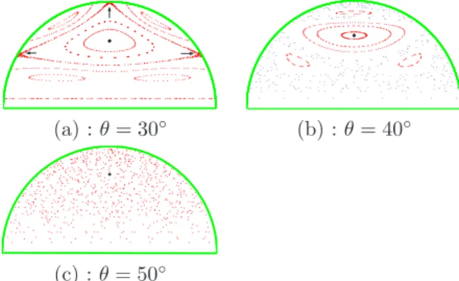
(a) : θ = 30◦ (b) : θ = 40◦
(c) : θ = 50◦
Fig. 3. Phase planes (Vr, |Vn|) for three wedge angle values.
The uncontrolled wedge billiard model we con-sider in this paper leads to stabilization problems of various complexity depending on the value of the angle θ. The variety of dynamical phenom-ena the wedge billiard displays as a function of the angle θ has been first studied by Lehtihet et al. (1986) (see also subsequent studies by Sz-eredi and Goodings (1993), Milner et al. (2001)). The value of the wedge angle determines in-tegrable, KAM (Kolmogorov-Arnold-Mauser, see Ott (1993) for an introduction) and chaotic re-gions in the phase space. Figure 3 depicts three phase planes (Vr, |Vn|) which illustrate the cases
θ < 45◦and θ > 45◦.
For θ < 45◦, the phase plane exhibits stable
and chaotic behavior associated with periodic points. As predicted by the KAM theory, stable fixed points are surrounded by encircling KAM curves forming near integrable regions called
is-land chains. Between these regions is a simply
connected domain of global chaos corresponding to collisions at the wedge vertex (Figure 3, (b)). An exception occurs at θ = 30◦ (Figure 3, (a))
where a structure of confined chaos (pointed by the arrows in (a)) is observed instead of global chaos. This local chaos originates from KAM be-havior rather than collisions at the vertex. For θ > 45◦, all the periodic fixed points turn out
that is all the phase plane is explored by the system state (Figure 3, (c)).
The configuration where θ > 45◦ is a
typi-cal example of chaotic billiard. In the last three decades, investigations of chaotic billiards became a popular research area in statistical mechanics. Wojtkowski (1998) proved that the uncontrolled elastic wedge billiard is hyperbolic. By hyperbolic behavior we mean the property of exponential di-vergence of nearby orbits. This property is closely tight to the ergodicity property according to which any trajectory will eventually come arbitrarily close to any periodic orbits of any desired period.
Period-one orbits
In the sequel, we focus on the stabilization of period-one orbits. Period-one orbits of the uncon-trolled wedge billiard are fixed points of the map
B (equation (7)) with µ = ˙µ = 0.
Fixed points are of the form ¡ ¯ Vr, | ¯Vn| ¢ = (0,1 + α2 α s 2 ¯E α2+ 3)
They characterize a one-parameter family of pe-riodic orbits, parametrized by their total energy
¯
E. These orbits exist for all wedge angle values.
They are represented by the + symbol in the phase planes of Figure 3. An illustration of the trace of a period-one orbit is given in Figure 4. Considering the eigenvalues λi, i = 1, 2 of the
2 ¯E g
√ 1+α2 3+α2
Fig. 4. Period-one orbit of the wedge billiard. linearized mapping of B around the period-one fixed points, we find that the fixed points are
elliptic (λ1 = 1
λ2 = e
±iu) when θ < 45◦ and
hyperbolic unstable (0 < λ1 < 1 < λ2) when
θ > 45◦.
4. LYAPUNOV-BASED CONTROL (θ < 45◦)
As depicted in Figure 3 (a) and (b), when the system is uncontrolled, the period-one fixed point is surrounded by a continuum of closed KAM curves forming an island chain. These curves are invariant, that is when the system initial state is on a curve, it keeps evolving on it according to the uncontrolled dynamics of the wedge billiard. This enforces the (Lyapunov) stability of the period-one fixed point.
The aforementioned KAM curves define the level set of a Lyapunov function.
Based on this observation and the hypothesis of stabilizability of the system at the equilibrium
point, we define a feedback control scheme based on the discrete analog of damping control (also known as as Jurdjevic-Quinn control, see Jurdje-vic and Quinn (1978)). Damping control assimi-lates the Lyapunov function to a ”system energy” and control is used to dissipate this energy, with the objective of rendering the equilibrium point asymptotically stable.
The closed KAM curves under consideration are obtained using numerical simulations. To set up the Lyapunov-based control design, we need an analytical parametrization of these curves. We approximate them with the level surfaces of an analytical Lyapunov function which is defined w.r.t. the linearized system around the period-one fixed point (see Appendix for details). Alternative methods (e.g. curve fitting) can be exploited to design analytical parametrizations of curves nu-merically defined.
The function expresses as follows :
V(Vr, Vn, E) = γVr2+(1−γ)(|Vn|−| ¯Vn|)2+(E− ¯E)2
where 0 < γ = 1−α2
(1+α2)2 < 1.
Figure 5 compares the closed KAM curves of the uncontrolled wedge billiard with the correspond-ing level surfaces of function V for two wedge angle values. In agreement with the small perturbation theory, the approximation quality increases as the system state evolves close to the equilibrium point. KAM curves Level surfaces θ = 30◦ KAM curves Level surfaces θ = 40◦ Fig. 5. Comparison of KAM curves (points) and
level surfaces of V for θ = 30◦, 40◦. Initial conditions are represented by squares (2). The equilibrium characterized by ¯Vr= 0, | ¯Vn| =
1+α2 α
q
2 ¯E
α2+3, E = ¯E3 is made asymptotically
stable using discrete-time damping control (Lee
3 When angular position is used for control, the controlled elastic wedge is conservative, the energy being conserved both during flight and through impacts. Hence equality
and Arapostathis (1988)). The resulting control law writes :
u[k + 2] = −²BT
i P A (x[k] − ¯x) (8)
where ² > 0 is a small control parameter and
i = 1, 2 according to angular position (u = µ) or angular momentum (u = ˙µ) actuation.
(A, P, Bi, i = 1, 2 are defined in the Appendix).
If the angular position is chosen for actuation (u = µ), the control law (8) can be saturated at an arbitrarily small constant magnitude to validate the small angle assumption.
Figure 6 illustrates the evolution of function V, for different wedge angle values, using damping control law (8) (with i = 2). Observe that V is not strictly monotonically decreasing, though sta-bilization of the period-one fixed point is effective.
0 5 10 15 20 25 30 35 40 0 0.2 0.4 0.6 0.8 1 1.2 1.4 V function value θ = 30° θ = 40° θ = 10° Fig. 6. Evolution of V
V(0)using angular momentum damping control. Wedge angles are equal to
θ = 10◦, 30◦, 40◦. The common initial condition is represented by the × symbol on the θ = 40◦ phase plane of Figure 5.
5. TRAPPING CONTROL (θ > 45◦)
Considering any unstable periodic orbit of the wedge billiard with θ > 45◦, the ergodicity
prop-erty ensures that any trajectory will eventually come arbitrarily close to the orbit. This offers the opportunity for controlling chaos : when the chaotic orbit approaches the unstable periodic orbit of interest it can be attracted to and main-tained on the orbit by applying small perturba-tions to the system. Controlling chaos was sug-gested by Ott et al. (1990), giving rise to the OGY method. Since the stabilization issue is based on a linear analysis of the system near a periodic orbit, standard results from linear control theory can be taken over directly.
Borrowing the (physicist) idea of controlling chaos, we first exploit the ergodicity property of the uncontrolled conservative wedge billiard. Sec-ond we design a state feedback controller using a pole placement method. The controller drives the angular position of one edge
µ[k + 2] = −k1(Vr[k] − ¯Vr) − k2(Vn[k] − ¯Vn) (9)
keeping the energy E of the controlled elastic wedge conserved. The closed-loop system is kept conservative.
The linear feedback law (9) achieves local asymp-totic stability of the equilibrium characterized by
¯ Vr= 0, | ¯Vn| =1+α 2 α q 2E α2+3.
Third, the basin of attraction of the linear con-troller is estimated.
The control methodology summarizes as follows. The wedge billiard is left uncontrolled until the trapping region of the linear controller is reached by the chaotic orbit. Applying the control law (9) asymptotically stabilizes the periodic orbit. A valid trapping region is obtained from the level sets of a quadratic Lyapunov function. To validate the small angle assumption, a maximum size for the trapping region is imposed. This saturates the magnitude of the angle deviation |µ|.
6. SIMULATION RESULTS
The control laws of Sections 3 and 4 are now briefly illustrated by simulation results.
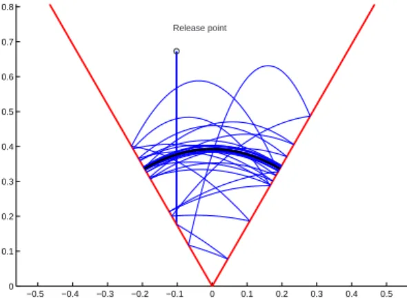
In the case θ < 45◦, we choose to stabilize the
period-one orbit characterized by the energy level ¯
E = 5.5J using angular momentum control ˙µ of
the left edge. The wedge angle is equal to θ = 30◦
and the initial conditions are chosen as |Vn[0]| =
−3.11m/s, Vr[0] = −|Vn[0]|m/s, E[0] = 1.2 ¯E,
which roughly corresponds to an initial drop of the ball. Figure 7 illustrates the trace of the ball trajectories. −0.5 −0.4 −0.3 −0.2 −0.1 0 0.1 0.2 0.3 0.4 0.5 0 0.1 0.2 0.3 0.4 0.5 0.6 0.7 0.8 Release point
Fig. 7. Trace of the trajectories
The case θ > 45◦ (here θ = 70◦) is illustrated
by the (Vr, |Vn|) phaseplane depicted on Figure
8. The system is initially left uncontrolled. Once the system state enters the basin of attraction (approximated by an ellipse) of the linear state feedback controller, the control law achieves sta-bilization of the equilibrium point.
−3 −2 −1 0 1 2 3 −0.5 0 0.5 1 1.5 2 2.5 3 3.5 4 v r |vn | (Vr,|Vn|) Phaseplane Initial condition Fig. 8. Phaseplane (Vr, |Vn|) 7. CONCLUSION
This paper has presented stabilization results for periodic orbits of the controlled wedge billiard, a model we view as an interesting benchmark for impact control stabilization problems. Two config-urations differing in the value range of the wedge angle have been addressed using two different control strategies. One exploits the ergodicity of the open-loop dynamics, the other uses the KAM curves surrounding the fixed point as candidate level set for a Lyapunov function. Both methods lead to simple and robust feedback laws with large basins of attraction.
REFERENCES
M. Buehler, D.E. Koditschek, and P.J. Kindl-mann. Planning and control of robotic juggling and catching tasks. International Journal of
Robotics Research, 13(2):101–118, April 1994.
R. R. Burridge, A. A. Rizzi, and D. E. Koditschek. Sequential composition of dynamically dexter-ous robot behaviors. International Journal of
Robotics Research, 18(6):534–555, June 1999.
V. Jurdjevic and J. Quinn. Controllability and stability. Journal of Differential Equations, 28: 381–389, 1978.
K. Lee and A. Arapostathis. Remarks on smooth feedback stabilization of nonlinear systems.
Systems and Control Letters, 10:41–44, 1988.
Lehtihet, H. E. Miller, and B. N. Numerical study of a billiard in a gravitational field. Physica, 21D:93–104, 1986.
K.M. Lynch and C.K. Black. Recurrence, con-trollability, and stabilization of juggling. IEEE
Trans. on Robotics and Automation, 17(2):113–
124, April 2001.
V. Milner, J.L. Hanssen, W.C. Campbell, and M.G. Raizen. Optical billiards for atoms.
Phys-ical Review Letters, 86:1514–1517, 2001.
E. Ott, C. Grebogi, and J.A. Yorke. Control-ling chaos. Phys. Rev. Lett., 64(11):1196–1199, 1990.
Edward Ott. Chaos in Dynamical Systems. Cam-bridge University Press, 1993.
A. A. Rizzi and D. E. Koditschek. Progress in spatial robot juggling. In IEEE International
Conference on Robotics and Automation, pages
775–780, Nice, France, 1992.
A. A. Rizzi and D. E. Koditschek. Further progress in robot juggling: The spatial two-juggle. In IEEE International Conference on
Robotics and Automation, pages 3:919–924,
At-lanta, GA, 1993.
R. Sepulchre and M. Gerard. Stabilization of periodic orbits in a wedge billiard. In IEEE
42nd Conf. on Decision and Control, pages
1568–1573, Maui, Hawaii-USA, 2003.
T. Szeredi and D.A. Goodings. Classical and quantum chaos of the wedge billiard. i. classical mechanics. Physical Review E, 48(5):3518–
3528, 1993.
Maciej P. Wojtkowski. Hamiltonian systems with linear potential and elastic constraints.
Funda-menta Mathematicae, 157:305–341, 1998.
A. Zavala-Rio and B. Brogliato. On the control of a one degree-of-freedom juggling robot.
Dy-namics and Control, 9:67–90, 1999.
APPENDIX
Linearized system
Considering the Jacobian linearization around the period-one fixed point
( ¯Vr, | ¯Vn|, ¯E) = (0, 1 + α2 α s 2 ¯E α2+ 3, ¯E)
of the controlled Poincar´e map B2on the actuated
wedge, we obtain : δx[k + 2] = Aδx[k] + B1µ[k + 2] + B2˙µ[k + 2] (10) where δx[k]= Ã Vr[k]− ¯Vr |Vn[k]|−| ¯Vn| E[k]− ¯E ! , A = Ã (8γ2−8γ +1) 4(1−γ)(2γ −1) 0 4γ(1−2γ) (8γ2−8γ + 1) 0 0 0 1 ! B1= Ã −2α ¯Vn 0 0 ! , B2= 2 ¯R 0 α sign( ¯Vn) 2α ¯R 1+α2V¯n α = tan θ, γ = 1−α2 (1+α2)2, ¯R = 2g1 ¡ 2(1 + α2) ¯E − α2V¯2 n ¢ The pair (A, B1) is controllable except when γ = 0
(square wedge billiard and θ = 90◦) and γ = 1/2
(θ ≈ 25.91◦).
The pair (A, B2) is controllable except when γ = 1
(⇔ θ = 0) and γ = 1/2 (θ ≈ 25.91◦).
Lyapunov Function
The quantityV(δx) = δxTP δx with P =
à γ 0 0 0 (1 − γ) 0 0 0 1 ! is a Lyapunov function for the system (10) because
P is a solution of the Lyapunov equation ATP A = P