HAL Id: hal-01867343
https://hal-ensta-bretagne.archives-ouvertes.fr/hal-01867343
Submitted on 4 Sep 2018
HAL is a multi-disciplinary open access
archive for the deposit and dissemination of
sci-entific research documents, whether they are
pub-lished or not. The documents may come from
teaching and research institutions in France or
abroad, or from public or private research centers.
L’archive ouverte pluridisciplinaire HAL, est
destinée au dépôt et à la diffusion de documents
scientifiques de niveau recherche, publiés ou non,
émanant des établissements d’enseignement et de
recherche français ou étrangers, des laboratoires
publics ou privés.
Radar Cross Section of Modified Target using Gaussian
Beam Methods: Experimental Validation
Ghanmi Helmi, Ali Khenchaf, Philippe Pouliguen
To cite this version:
Ghanmi Helmi, Ali Khenchaf, Philippe Pouliguen. Radar Cross Section of Modified Target using
Gaussian Beam Methods: Experimental Validation. International conference on Radar 2018, Aug
2018, Brisbane, Australia. �hal-01867343�
Radar Cross Section of Modified Target using
Gaussian Beam Methods: Experimental Validation
H. Ghanmi, A. Khenchaf
Lab-STICC UMR CNRS 6285, ENSTA Bretagne 29806, Brest, France
[email protected] & [email protected]
P. Pouliguen
French General Directorate for Armament (DGA) 75509, Paris, France
Abstract—The aim of this paper is to study the Radar Cross
Section (RCS) of modified radar targets (plate with notch) using Gaussian Beam techniques. The Gaussian methods used in this work are Gaussian Beam Summation (GBS) and Gaussian Beam Launching (GBL). We establish the theoretical formulation of the GBS and GBL techniques and analyze the influence of the main Gaussian beam parameters on the variation of the scattered field. Then, we present the simulations of RCS. The numerical results are compared with PO, MoM methods, and also with experimental measurements performed in the anechoic chamber at Lab-STICC (ENSTA Bretagne).
Keywords—Radar Cross Section (RCS); Gaussian Beam Summation (GBS); Gaussian Beam Launching(GBL); Physical Optic (PO); Method of Moment (MoM); Physical Theory of Diffraction (PTD)
I. INTRODUCTION
The RCS can be simulated using rigorous methods such as Method of Moment (MoM), Finite Difference Time Domain (FDTD) or asymptotic models including Geometrical Optics (GO), Physical Optic (PO), Physical Theory of Diffraction (PTD), and Geometrical Theory of Diffraction (GTD). The rigorous methods like MoM are based on an integral formulation, and they are served to validate the new asymptotic approach. The asymptotic approach reduces the operation number of solving of high-frequency equations for large objects [1], [9], [10]. The asymptotic methods using the hypothesis of locally plane wave and high-frequency approximation are based on the principle of rays. The application of the type of these methods in a complex propagation scenario is regularly limited by the transaction between highlighted and shadowed region and the caustic problem (except the PO method). The visibility of these limitations depends on the complexity of the radar target and the geometric observation configuration. For these reasons we chose to apply two asymptotic techniques based on Gaussian beams called Gaussian Beam summation (GBS) and Gaussian Beam Launching (GBL), and we study the RCS variation of different radar targets. In the GBL technique, when a radar target is illuminated by a Gaussian Beam, the field radiated is decomposed into a plane wave spectrum then summing the contribution of the radiations of all the beams interacting with the target [11]. The Gaussian Beam summation as an asymptotic approach for computing high-frequency wave fields was developed by V. Cerveny and M.M. Popov [2]-[5]. The
summation of Gaussian beams allows solving some critical points of the asymptotic ray methods such as the problems related to the evaluation of wave field in singular areas. In addition, the Gaussian beams summation method offers a solution to overcome the caustics problem [3], [4], [13]-[15].
In this context, the objective of this work is to investigate the different mechanisms of electromagnetic wave scattering by a modified radar targets (plate with notch) using GBS and GBL methods and validate the numerical simulation results by experimental measurements.
II. FORMULATION
A. GBS method: formulation
The Gaussian Beam method used for the estimation of a wave field in high-frequency approximation has been developed by V. Cerveny [4], [8] and M.M. Popov [6]. The approach is based on the summation of Gaussian beams. This physical principle of Gaussian Beam approach consists in a compatible step assembly. Consider a homogeneous and isotropic medium and an electromagnetic wave propagating in this medium which is acting excited by a point source. In the GBS method, the total field at the receiver is a sum of the contributions of all the beams passing in the vicinity of the receiver (which is the same case for each observation point). For each considered ray, we determine a Gaussian beam propagating along the ray. Then we sum the contribution of each Gaussian beam to the receiver overall rays [8], [9].
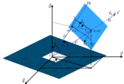
Fig. 1. Geometric configuration and coordinate parameters for Gaussian Beam Summation (GBS) formulation. Plate with a rectangular aperture (notch).
Fig. 1 presents the ray-centered coordinate system (s, q1, q2)
amplitude u(s, q1, q2, t). This coordinate system is connected to
any selected Ω radius. In addition to the geometric parameters, assumptions are also used to establish the theoretical equation of GBS. In fact, we start by considering a homogeneous and isotropic medium an electromagnetic wave propagating (with a propagation velocity v) in this medium which is being excited by a point source. Then, we suppose that some wave process is described by the Helmholtz’s wave equation and the point source is positioned in the origin. After, we solve the Helmholtz’s equation in the neighborhood of rays. Using the local coordinates and at the receiver point, the solution of the Helmholtz equation as a solitary Gaussian beam is given by (1) [2], [3]: ( ) [ ] ( )
(
)
( ) 1 2 1 1 2 1 , , , exp det 2 T s v u s q q t j t s q P Q q Q ds s v ω τ τ − = ⋅ − − − ⋅ ⋅ ⋅ =
(1)In (1), v represents the propagation velocity; qT is the transpose of the vector; the travel time from the source along the designated ray is represented by τ(s), and the other parameters are cited in the previous paragraph. The parameters Q and P (which depend on s) are two-by-two matrix named “dynamic quantities” [3], [12] which are related by the “Dynamic Ray Tracing” (DRT) (2).
= . ; =0 ds dP and P c ds dQ (2)
The system of differential equations (2), is solved by introducing initial conditions specified at an arbitrary point (s = s0) on the central ray. The initial conditions are also related to a
three others conditions along the whole rays [6] which are: even though P and Q are not symmetrical the (P×Q-1) must be
symmetric matrix; Im(P×Q-1) is a positive-definite matrix and
(det[Q]≠ 0).
The initial values of Q and P can be established by using Hill’s initial data for the Green’s function [6], [7]:
0 2 0 . ; . ; . I and s s c j P I c Q=ωrω = = (3)
In (3) ω0 denotes the beginning half beam width at a
frequency f = ωr/2π. I is the identity matrix (2×2). Using the
initial conditions in (3), we can find the general solution of (2), and can be written as follows:
(
)
I c j P and I s s j c Q r. . . . ; . 0 2 0 = − + = ω ω (4) In the case of homogeneous media, by using (4) in (1), wereturn to the representation of the amplitude u of the Gaussian beam in 3D: ( ) ( ) ( ) ( ) ( ) − + − + + − + = 0 2 0 2 2 2 1 0 2 0 2 3 2 1 . . . 2 1 exp . . . , , s s c j c q q s j s s j c q q s u ω ω τ ω ω ω (5)
Using the geometrical configuration illustrated in Fig. 1, and introducing the spherical coordination system (r, θ, φ), we
can deduce the following factor (in 6) as function of the distance (r) from the transmitter to the receiver:
.sin
( )
ϕ; 0 .cos( )
ϕ 2 2 2 1 q r and s s r q + = − = (6)Finally, to calculate the full amplitude (uGBS) at the receiver
we must use an integral formulation as shown in equation (7). This integral will be calculated on all Gaussian beams described by their characteristic angle (called takeoff angle φ) from the source:
(
)
. , 1, 2 . G B S s q q d u ϕu γ ϕ γ =Φ(7)
In (7) the integral function is the product of three terms. The first term denoted Φϕ is the complex weight function
which may differ from ray to ray, however, remains constant in each considered ray. The second term is the function uφ(s, q1,
q2) is the Gaussian beam related to the ray given by (5).
Finally, the third term dγ is expressed according to angle φ by the equation (2π .sin(φ).dφ). The choice of the integration domain γ is related to the function of the Gaussian beam uφ(s,
q1, q2) and to the central ray. In fact, the domain γ is fixed on
the central ray and delimits the Gaussian beams propagating in the neighbor of the central ray. On the other hand, the contribution of the Gaussian beams uφ(s, q1, q2) is conditioned
by the fact that outside the γ domain do not contribute effectively to the wave field.
For a homogeneous medium, the ray asymptotic solution of the Helmholtz equation is given by the following equation:
( )
1 exp 4 u r j r r c ω π = ⋅ ⋅ (8) The GBS integral, in (7), may be evaluated asymptotically using the saddle-point method. Therefore, this result must match with the ray asymptotic solution (8) in the regular area. The calculation of the complex weight functionΦϕ is performed by matching the asymptotic solution of (7) and (8). This integral of GBS is evaluated and simulated numerically and quadratically by a regular increment denoted Δφk.N
( )
k k k k k GBS u u = π
Φϕ ϕ ϕ Δϕ = . sin . . . . 2 1 (9) The formulation in (9) will be used to compute the scattered field, then the RCS using GBS method.After the formulation of the scattered filed using GBS method ((7) and (9)), we examine the effect of the main parameters of the Gaussian beam on the variation on the field amplitude. Then, we compare the solution based on Gaussian beam with the analytical solution given by (8). The principal influencing parameters in GBS method in (7) are the number (N) of beams and their width value (ω0). To verify the validity
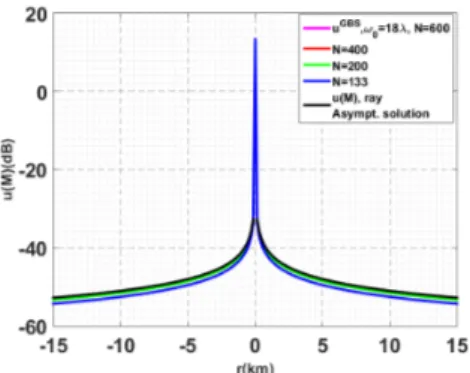
of the proposed method, we analyze the behavior of GBS solution for different value of beam width and beam number. Fig. 2 compares the amplitude of field calculated ray asymptotic solution of the Helmholtz equation and GBS method, for a frequency equal to 10GHz, a beam width (ω0)
equal to 18λ (where λ is the wavelength) and for various beams number (N){133, 200, 400 and 600}. This simulation (Fig. 2) has been realized as a function of the distance (r in km) from
the source to the receiver. We can observe, when the number of beams is more than 200, the GBS and the ray asymptotic are in are almost identical. Thus, a high beam number is necessary for high precision, which is the same case of the classical ray tracing methods.
Fig. 2. Comparison between the ray asymptotic solution and the Gaussian beam summation method for N=133, 200, 400, 600 the beam width is 18λ.
Fig. 3. Variation of percentage error between GBS method and ray asymptotic solution as function (r) and for several beam number.
Fig. 3 illustrates the variation of percentage error between GBS method and ray solution for different beam density. We can see that for sufficient beam density, N=600, the relative error remains below 3% even at 15 km from the source. In addition, one should note that in r=0 the simulation based on GBS method do not have singularities, which is contrary to the ray asymptotic method. This result confirms that by using the GBS method we can overcome some limitation of the ray asymptotic models.
B. GBL method: formulation
The Gaussian Beam Launching (GBL) technique has been introduced and applied in the research published by H. T. Chou [11]. Consider a target (plate, disc, cylinder,…) illuminated by a Gaussian beam, the GBL method is applied to calculate the radiation integral of the target scattered fields. For the considered Gaussian beam, the incident magnetic field is given by the following form [11], [14]:
( ) ( )0 i i exp 2i i2 i i i i i i i i i i jb x y H H jk z z jb z jb ρ ρ = +ρ++ − + +ρ++ (10)
In (10), the distance between a point on the illuminated surface and the waist the incident Gaussian beam is denoted by
ρi, the position vector in the Gaussian beam is defined by and
bi =k.ω02/2, and k, ω0 are the wave number and the half
beam-width respectively.
The electric fields scattered from the target surface (Σ) illuminated by the incident beam is given by the integration of the incident Gaussian beam on the reflector surface (PO integral). This integral is written by (11):
( ) . 0 .
(
( ))
exp( . . ). 4. i z i i r j k R Z j k E r R R e H r ds R π Σ ε − = × × ×
(11)Finally, by using (10) in (11) and solving the integral, we can compute the scattered field applying GBL formulation as in [11].
In both GBS and GBL method, it’s required to take into account the far field approximation parameters (distance r, target size D and wave length λ). In order that the phases and amplitudes of the waves arriving from different regions of the target do not vary considerably with the distance (r), the far-field region must be far enough away from the source. This region of the far field starts at a distance "r" given by the following equation (Fraunhofer criterion) [16] : r ≥ ((2.D2)/λ).
Fig. 4. Target size as the function of distance for far-field approximation: the Far-field criterion of Fraunhofer.
Fig. 4 shows the minimum far-field range as a function of the target dimensions D, and for different frequencies values. In this work, all simulations and measurements are realized in the frequency equal to10GHz.
III. NUMERICAL AND EXPERIMENTAL RESULTS: VALIDATION AND EVALUATION
A. Measuring devices and considered targets
The validation of the numerical simulation results have been done in the monostatic configuration (where the transmitter and the receiver are in in the same position), which is located in an anechoic chamber (8m × 5m × 5m) at ENSTA Bretagne (see Fig. 5).
(b) (c)
Fig. 5. (a) General description of the experimental setup, (b) flat plate, (c) plate with an aperture.
The characteristics of various components of measurements system are: All walls are covered with absorbent material. A computer controls the Vectorial Network Analyzer (Anritsu 37347D) which operates in the frequency range from 40MHz to 20GHz and the positioning system. An elevation motor for adjusting the height of the target. The NEWPORT positioning system with an angular resolution equal to 0.01° and an angle vary between -90° and 90°.
The dimensions of the metallic plate and it notch are shown in Fig. 6(a), this target will be used for experimental measurements. The size of the plate and its rectangular notch are (30cm × 30cm) and (15cm × 15cm) respectively. The geometry of the considered radar target (plate with notch) meshed with a triangular patch (using CATIA software) is present in Fig. 6(b). In this numerical model of the radar target, each facet is represented by a triangle node (in blue), it centered in red color (bright points) and black cross in the middle of the external edge and also in the notch edge. The RCS of the plate with an aperture includes the surface scattered field and the edge diffracted field (by the notch and the external of the plate). In the GBS method, to consider the edge diffraction contribution, we have chosen to use the physical theory of diffraction (PTD) method which is detailed in [1]. In fact, PTD method is used to compute a diffraction part for each ray that hits the target surface in the vicinity of an edge and is calculated in the complex weight function in the integral (7).
(a) (b)
Fig. 6. (a) Dimensions and (b) mesh of PEC plate with an aperture.
The next part presents the comparison between numerical and experimental RCS results. Firstly the study the RCS of a PEC flat plate is exposed. Then the influences of the presence of the rectangular aperture on the RCS variations are displayed. B. RCS estimation: numerical and experimental results
To validate the simulation results obtained using the Gaussian techniques (GBS, GBL), the variation of the RCS of a squared PEC flat plate (size = 10λ×10λ) in the monostatic case is measured in an anechoic chamber firstly. Then a comparison is also performed with others numerical
approaches. The measurements are performed at a frequency of 10GHz, the numerical simulation parameters are fixed as follows: beam width of ω0 =2λ, beam number equal to 200,
azimuth angle ϕi=0° and an incident angle −80˚ < θi < 80˚.
Fig. 7. Comparison between GBS+PTD, GBL, PO, MoM methods and experimental measurements in vv polarization: PEC flat plate, f =10GHz.
In Fig. 7, we compare the GBS+PTD and GBL+PTD with the experimental measurements and the numerical models (PO, MoM in FEKO software). It is observed that, when the diffraction contributions are accounted, the combined GBS+PTD and GBL+PTD methods give an accurate qualitative representation of the RCS variation for all observation angles. We can also remark that PO is insufficient in computing of edge plate diffraction contributions, although the agreement of GBS+PTD and GBL+PTD with the rigorous MoM solution and measured data are good in the most of scattering angles. These results will serve as a benchmark for analysis of the influence of the presence of the notch in the RCS variations.
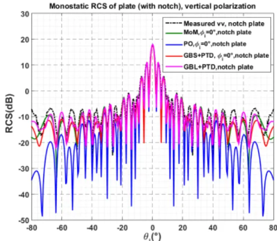
Fig. 8. Comparison between GBS+PTD, GBL+PTD, MoM, PO methods and experimental measurements in vv polarization: PEC plate with notch, f =10GHz, ϕi=0°.
Fig. 8 shows the RCS of a PEC plate with rectangular notch obtained using (GBS+PTD, GBL+PTD, MoM, PO) methods and experimental measurement (same parameters in Fig. 7). It is observed that for the incident between 0° and 20°, the numerical models and experimental results are in good
30cm 30 cm 15cm 15 cm
agreement. However, in the case of the angle close to 80°, a difference appears between the different curves of RCS. Secondly, we can see that for the scattering angle larger than 35°, the RCS curves using GBS+PTD and GBL+PTD are near to those obtained by MoM method and measurement, but higher than the PO model which may be related to the diffraction of the edge of notch and external of the plate.
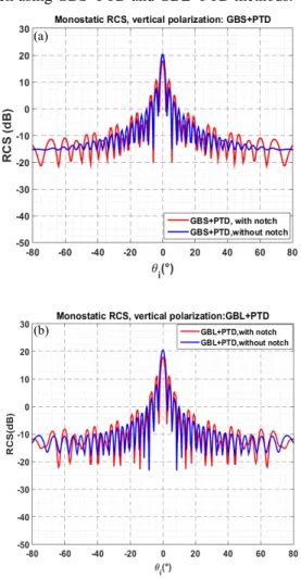
To obtain more information about the impact of the notch of the plate, we compare in the RCS of a PEC with and without notch using GBS+PTD and GBL+PTD methods.
Fig. 9. Comparison between RCS of a flat plate and a plate with notch: f =10GHz, ϕi=0°, (a) GBS+PTD, (b) GBL+PTD.
Fig. 9 shows a comparison between RCS of a flat plate (in blue) and a plate with a notch (in red). It is observed, the effect of the presence of notch on the RCS curve is depending on the value of incident angle. In fact, at θi = 0° the amplitude of RCS
decrease, nonetheless for the others incident angle values the RCS of a flat plate is regularly lower than that of the plate with a notch.
IV. CONCLUSION AND FUTURE WORK
In the present paper, new techniques in the electromagnetic scattering from a modified canonical radar target (flat pale with notch) have been applied. The GBS and GBL methods used in this work are based on the Gaussian beams. In the GBS technique, the total field at the receiver is epitomized by the
integral over all Gaussian beams passing in the vicinity of the receiver. In the GBL method, when a target is illuminated by a Gaussian beam, the radiated field is calculated by decomposing it into a plane wave spectrum and then summing the contributions of the radiations of all beams interacting with the target. In addition, to take into account the edge diffraction of the aperture and the external part of the plate, GBS and GBL methods have been combined with the Physical Theory of Diffraction (PTD). The numerical and experimental results show that the two methods GBS and GBL model well the variation of the field radiated by a modified canonical target (plate with an aperture). To extend the applications of the GBS and GBL, one of the perspectives of the presented work is to study the RCS of dielectric targets by using the GBS/GBL methods.
ACKNOWLEDGMENT
The authors wish to thank the DGA (Direction Générale de l’Armement, France)-MRIS for its support of the SOFAGEMM project, where this work is in Progress.
REFERENCES
[1] F.Weinmann, “Ray tracing with PO/PTD for RCS modeling of large complex objects,” IEEE Ant Prop, vol. 54, no. 6, pp. 1797–1806, 2006. [2] V. Červený, “Summation of paraxial Gaussian beams and of paraxial ray
approximations in inhomogeneous anisotropic layered structures,” In Seismic waves in Complex 3-D Structures, no. 10, pp. 121–159, 2000. [3] M. M. Popov, “A new method of computation of wave fields using
Gaussian beams,” Wave Motion., vol. 4, pp. 85-97, 1982.
[4] V. Červený, “Expansion of a Plane Wave into Gaussian Beams,” Stidia geoph. And geod., vol. 26, pp. 120 - 131, 1982.
[5] V. Červený, “Seismic Ray Theory,” Cambridge: Cambridge Press, 2001. [6] V. Červený, “Computation of wave field in homogeneous media,”
Geophys. J. R. astr. Soc., vol. 70, pp. 109-128, 1982.
[7] N. R. Hill, “Gaussian beam migration,” Geophysics, vol. 55, no.11, pp. 1416-1428, 1990.
[8] B. S. White, A. Norris, A. Bayliss and R. Burridge, “Some remarks on the Gaussian beam summation method,” Geophysical Journal of the Royal Astronomical Society, vol. 89, pp. 579-636 , 1987.
[9] H. T. Chou and P. H. Pathak, “Uniform asymptotic solution for electromagnetic reflection and diffraction of an arbitrary Gaussian beam by a smooth surface with an edge,” Radio Science, vol. 32, no.14, pp. 1319-1336, 1997.
[10] P. Pouliguen, L. Lucas, F. Muller, S. Quete and C. Terret, “Calculation and analysis of electromagnetic scattering by helicopter rotating blades,” IEEE Trans. Ant. Prop, vol. 50, no. 10, pp. 1396-1408, 2002.
[11] H. T. Chou, P. Pathak et R. J. Burkholder, “Novel Gaussian Beam Method for the Rapid Analysis of Large Reflector Antennas,” IEEE Trans Antennas and Propagation, vol. 49, n° 16, pp. 880-893, 2001. [12] B. Bleistein, “Mathematics of Modeling, Migration and Inversion with
Gaussian Beams,” Colorado, USA, 2008.
[13] M. Katsav and E. Heyman, “Gaussian Beam Summation Representation of Beam Diffraction by an Impedance Wedge: A 3D Electromagnetic Formulation Within the Physical Optics Approximation,” IEEE Trans. Antennas Propagation, vol. 60, no. 12, pp. 5843-5858, 2012.
[14] P.O. Leye, A. Khenchaf, and P. Pouliguen, “The Gaussian Beam Summation and the Gaussian Launching Methods in Scattering Problem,” J. Elect. Analysis and Applications, vol. 8, pp.219-225, 2016. [15] H. Ghanmi, A. Khenchaf, P. Pouliguen and P. O. Leye, “Study of RCS
of complex target: Experimental measurements and Gaussian beam summation method,” IEEE CAMA conference, pp. 196-199, 2017. [16] Warren L. Stutzman, Gary A. Thiele. “Antenna Theory and Design”.
John Wileys & Sons, Inc., 1997. (a)