L'ÉTUDE DES CHANGEMENTS APPRÉHENDÉS DES PRÉCIPITATIONS EXTRÊMES SUR LA PROVINCE DU QUÉBEC EN UTILISANT UN
ENSEMBLE DE MULTI-MRC
MÉMOIRE PRÉSENTÉ COMME EXIGENCE PARTIELLE
DE LA MAÎTRISE EN SCIENCES DE L'ATMOSPHÈRE
PAR
ANDRÉ MONETTE
Avertissement
La diffusion de ce mémoire se fait dans le' respect des droits de son auteur, qui a signé le formulaire
Autorisation de reproduire.
et de diffùser un travail de recherche de.
cycles
supérieurs (SDU-522- Rév
.01-2006). Cette autorisation stipule que «conformément·à l'article 11 du Règlement no 8 des études de cycles supérieurs, [l'auteur] concède à l'Université du Québecà
Montréal une lic~nce non exclusive d'utilisation et de . publication oe la totalité ou d'une partie importante de [son] travail de recherche pour des fins pédagogiques et non commerciales. Plus précisément, [l'auteur] autorise l'Université du Québec à Montréal à reproduire, diffuser, prêter, distribuer ou vendre des .· copies de. [son] travail de rechercheà
des fins non commerciales sur quelque support que ce soit, y compris l'Internet. Cette licence et cette autorisation n'entraînent pas une renonciation de [la] part [de l'auteur]à
[ses] droits moraux ni à [ses] droits de propriété intellectuelle. Sauf entente contraire, [l'auteur] conserve la liberté de diffuser et de commercialiser ou non ce travail dont [ill possède un exemplaire .. »dévouement et son encadrement durant ce projet. Je voudrais aussi souligner la contribution substantielle de mon co-directeur de recherche, Naveed Khaliq, pour sa précieuse expertise sur la méthode statistique de ce projet. Évidemment, sans l'appui financier du projet RDC, du CRSNG, d'Hydro-Québec et d'OURANOS, et des simulations du projet NARCCAP, ce projet n'aurait pu existé. Finalement, je voudrais remercier mes collègues à l'UQÀM pour leur aide et support, particulièrement Bratislav Mladjic et Debasish Pai Mazumder.
LISTE DES FIGURES ... vii
LISTE DES TABLEAUX ... vii
LISTE DES ACRONYMES ... xv
LISTE DES SYMBOLES ... x
RÉSUMÉ ... xi
CHAPITRE! INTRODUCTION ... 1
CHAPITRE II PROJECTED CHANGES TO PRECIPITA TI ON EXTREMES FOR NORTHEAST CANADIAN WATERSHEDS USING A MULTI-RCM ENSEMBLE ... l l Abstract ... 12
2.1. Introduction ... 13 2.2. Simulations and observations ... 15
2.2.1. NARCCAP simulations ... 15
2.2.2 Observed data ... 16
2.3. Methodology ... 17
2.3.1. Reference grid ... 17 2.3.2. Precipitation characteristics and their estimation ... 17
2.3.3. Performance and lateral boundary forcing errors ... 19
2.3.4. Structural and AOGCM related uncertainties ... 19
2.4. Results ... 21
2.4.1. Statistical homogeneity analysis ... 21
2.4.2. Performance and boundary forcing errors ... 22
2.4.3. RCMs structural and AOGCM related uncertainties ... 24
2.4.4. Projected changes ... 25
2.5. Summary and conclusions ... 27
Acknowledgements ... 29 FIGURES ... 30 TABLEAUX ... 43 CHAPITRE III CONCLUSION ... 47 ANNEXE A FIGURES SUPPLÉMENTAIRES N'AYANT PAS ÉTÉ PRÉSENTÉES DANS L'ARTICLE, MAIS DISCUTÉES DIRECTEMENT OU INDIRECTEMENT ... 53
ANNEXEE TABLEAUX SUPPLÉMENTAIRES N'AYANT PAS ÉTÉ PRÉSENTÉS DANS L'ARTICLE, MAIS DISCUTÉS DIRECTEMENT OU INDIRECTEMENT ... 67
LISTE DES FIGURES
Figure Page
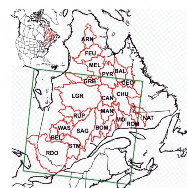
2.1 Study region with its 21 watersheds (see Table 2 for details) overlaid with the reference grid. The domain of gridded observed daily precipitation data is shown in green. The inset shows the location of the study region in North
America ... 31
2.2 Observed regional return levels (in mm) of 10-, 30- and 50-yr return period for 1-, 3- and 7-day precipitation extremes for the reference 1980-2000 period for 14 ofthe 21 watersheds ... 32
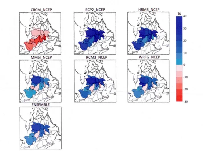
2.3 Relative difference between Q(I,IO) derived from NCEP-driven RCM simulations and observed dataset for 14 of the 21 watersheds for the reference 1980-2000
period. Ensemble averaged differences are also shown ... 33
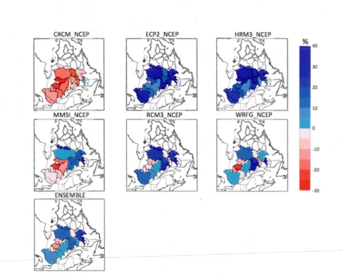
2.4 Relative difference between Q(7,50) derived from NCEP-driven RCM simulations and observed dataset for 14 of the 21 watersheds for the reference 1980-2000 period. Ensemble averaged differences are also shown ... 34
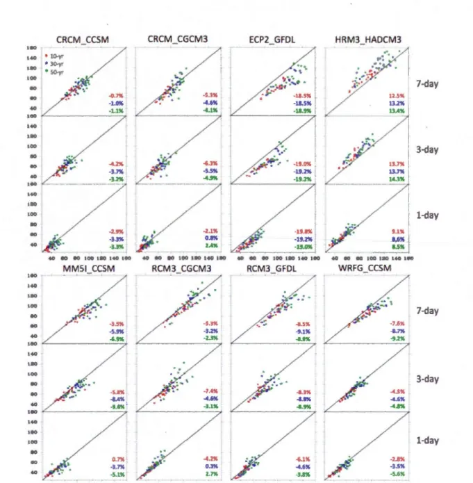
2.5 Scatter plots of 10-(red), 30-(blue) and 50-yr (green) return levels (in mm) of 1-, 3- and 7-day precipitation extremes for the 1980-2000 period. X-axis corresponds to NCEP driven RCM simulation, white y-axis corresponds to AOGCM driven simulation. Numbers in each panel represent average
percentage difference between NCEP and AOGCM driven simulations ... 35
2.6 Coefficient ofvariation ofNCEP-driven RCM simulations for 10-, 30- and 50-yr regional return levels ofl-, 3- and 7-day precipitation extremes ... 36
2.7 Ensemble averaged projected changes (in%) to 10-, 30-and 50-yr regional return levels of 1-,3-and 7-day precipitation extremes for future 2041-2070
period with respect to the current 1971-2000 period ... 3 7
2.8 Projected changes (in%) to 10-, 30- and 50-yr regional return levels of 1-, 3 -and 7-day precipitation extremes for future 2041-2070 period with respect to
the current 1971-2000 period for CRCM_CCSM ... 38
2.9 Projected changes (in%) to 10-, 30- and 50-yr regional return levels of 1-, 3 -and 7-day precipitation extremes for future 2041-2070 period with respect to
the current 1971-2000 period for CRCM_CGCM3 ... 39
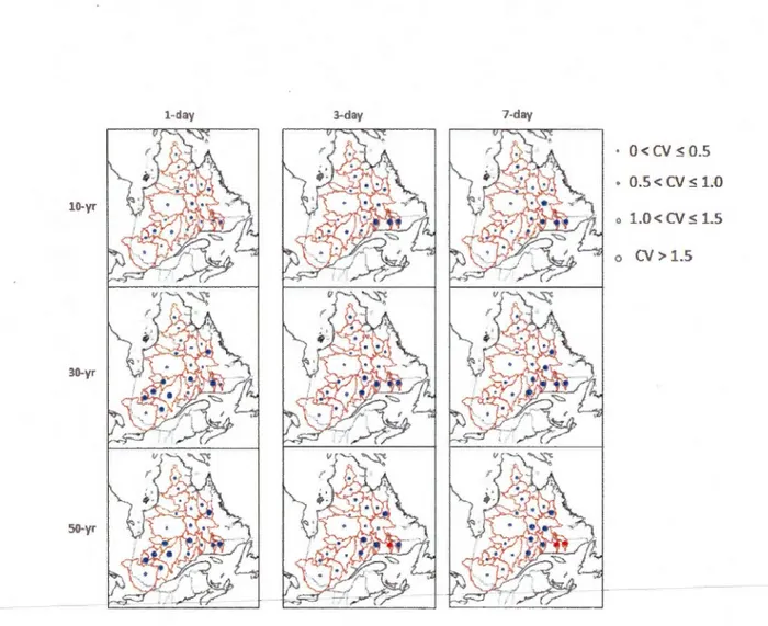
2.10 Coefficient of variation of projected changes to 10-, 30- and 50-yr regional return levels of 1-, 3- and 7-day precipitation extremes based on the multi-RCM ensemble. Blue (red) dots are used for watersheds with positive (negative)
projected ensemble averaged changes ... .40
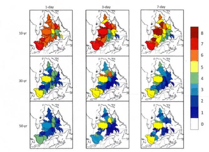
2.11 Number of AOGCM/RCM simulation pairs (out of eight) that predict a
significant change (at 5% leve!) for 10-, 30- and 50-yr regional return levels of 1-, 3-and 7-day precipitation extremes ... .41
2.12 Number of AOGCM/RCM simulation pairs (out of eight) that predict a
significant change (at 10% leve!) for 10-, 30-and 50-yr regional return levels of 1-, 3-and 7-day precipitation extremes ... .42
A.1 Number of extreme precipitation duration cases, out of six
(i.e. 1-, 2-, 3-, 5-, 7-, and 10-day precipitation extremes), for which a basin
is found homogeneous using the observed data. Same information for the case of six RCM NCEP simulations is shown in brackets ... 54
A.2 Observed regional return levels (in mm) of lü-, 3ü-and 5ü-yr return period for 2-, 5-and lü-day precipitation extremes for the reference 198ü-2üüü period
for 14 of the 21 watersheds ... , ... 55
A.3 Relative difference between Qc2,Io) derived from NCEP-driven RCM simulations and observed dataset for 14 ofthe 21 watersheds for the reference 198ü-2üüü
period. Ensemble averaged differences are also shown ... 56
A.4 Relative difference between Q(Io,so) derived from NCEP-driven RCM simulations and observed dataset for 14 of the 21 watersheds for the reference 198ü-2üüü
period. Ensemble averaged differences are also shown ... 57
A.5 Scatter plots of lü-(red), 3ü- (blue) and 5ü-yr (green) return levels (in mm) of2-, 5-and lü-day precipitation extremes for the 198ü-2üüü period. X-axis
corresponds to NCEP driven RCM simulation, while y-axis corresponds to AOGCM driven simulation. Numbers in each panel represent average percentage difference between NCEP and AOGCM driven simulations ... 58
A.6 Coefficient of variation ofNCEP-driven RCM simulations for lü-, 3ü- and 5ü-yr regional retum levels of2-, 5- and lü-day precipitation extremes ... 59
A.7 Ensemble averaged projected changes (in%) to 10-, 3ü- and 5ü-yr regional return levels of2-, 5- and lü-day precipitation extremes for future 2ü41-2ü7ü period with respect to the current 1971-2üüü period ... 6ü
A.8 Projected changes (in%) to lü-, 3ü- and 5ü-yr regional retum levels of2-, 5-and lü-day precipitation extremes for future 2ü41-2ü7ü period with respect to the current 1971-2üüü period for CRCM_CCSM ... 61
-A.9 Projected changes (in%) to 10-, 30-and 50-yr regional return levels of 2-, 5-and 10-day precipitation extremes for future 2041-2070 period with respect to the
current 1971-2000 period for CRCM_CGCM3 ... 62
A.1 0 Coefficient of variation of projected changes to 10-, 30- and 50-yr regional return levels of2-, 5-and 10-day precipitation extremes based on the multi-RCM ensemble. Blue (red) dots are used for watersheds with positive (negative)
projected ensemble averaged changes ... 63
A.11 Number of AOGCM/RCM simulation pairs (out of eight) that predict a significant change (at 5% level) for 10-, 30- and 50-yr regional return levels
of2-, 5-and Lü-day precipitation extremes ... 64
A.12 Number of AOGCM/RCM simulation pairs (out of eight) that predict a significant change (at 10% level) for 10-, 30-and 50-yr regional return levels
RCM simulations considered in this study ... 44
2.2 Description ofthe 21 watersheds used in the study ... 45
2.3 Percentage of stastically significant changes for 10-, 30-and 50-yr regional retum levels of 1-, 3-, and 7-day precipitation extremes at the 95% leve! (90%
leve! in parenthesis) ... 46
CRCM CGCM3
co2
cv
ECP2 GCM GEV GFDL GIEC GLO GNO GPA HadCM3 HRM3 IPCC MCG MMSI MRC NCEPCanadian Regional Climate Mode!
Canadian Global Climate Mode! version 3
Dioxyde de Carbone
Coefficient de Variation 1 Coefficient ofVariation
Experimental Climate Prediction centre regional mode! 2
Global Climate Model
Generalized Extreme Value
Geophysical Fluid Dynamics Laboratory
Groupe d'experts Intergouvernemental sur l'Évolution du Climat
Generalized Logistic
Generalized Normal
Generalized Pareto
Hadley Centre Coupled Mode!, version 3 Hadley Regional Mode! 3
Intergovernemental Panel on Climate Change
Modèle de Circulation Générale
MM5 - PSU/NCAR Mesoscale Mode!
Modèle Régional du Climat
NARCCAP NCAR PE3 RFA RCM RCM3
SRES
UQAM WRFGNorth American Regional Climate Change Assessment Program National Center for Atmospheric Research
Pearson Type 3
Regional Frequency Analysis Regional Climate Mode!
Regional Climate Mode! version 3 Special Report on Emissions Scenarios Université du Québec à Montréal Weather Research & Forecasting mode!
Q
z
T
d
Quanti le
Z goodness-of-fit test statistic
Période de retour (années)
période de référence (1971-2000). Pour ce faire, un ensemble de multi-modèles régionaux du climat (MRC) provenant du North American Regional Climate Change Assessment Program est utilisé. Le projet comprend six MRC piloté par les ré-analyses II NCEP couvrant la période 1980-2004 et piloté par quatre modèles de circulation générale de l'atmosphère (MCGA) couvrant une période de référence (1971-2000) et future (2041-2070). L'analyse fréquentielle régionale est choisie comme méthode pour développer les niveaux de retour des précipitations extrêmes pour des périodes de retour de 10, 30 et 50 années.
L'étude comporte une évaluation de la performance des six différents MRC liée aux différences dans leurs composantes physiques et dynamiques ainsi qu'une évaluation de l'effet du choix des conditions aux frontières de type ré-analyses par rapport à de type MCGA. Les résultats suggèrent que les différences liées aux composantes internes des MRC sont plus importantes que celles liées au choix des conditions aux frontières. D'autre part, par l'utilisation d'un ensemble de multi-MRC et du coefficient de variation, une quantification des incertitudes liées à la structure interne du MRC et du choix MGCA comme pilote est possible. En général, les incertitudes liées à la structure interne des MRC sont plus importantes que celles liées au choix du MGCA pour les bassins versants et les variables de cette étude.
L'analyse des changements appréhendés dans les niveaux de retours des précipitations extrêmes suggère une augmentation pour la majorité des bassins et des combinaisons à l'étude (durée et période de retour). Les plus petites augmentations ainsi que les plus grandes incertitudes se retrouvent dans les bassins au sud-est du Québec. Au contraire, les plus grandes augmentations et les plus faibles incertitudes se retrouvent dans les bassins nordiques.
Une augmentation dans les niveaux de retour des précipitations extrêmes a des conséquences importantes sur la gestion et la conception des infrastructures existantes et futures, spécialement pour cette région du Canada où la production d'énergie hydro-électrique est omniprésente.
Les changements climatiques font maintenant consensus dans la communauté scientifiques. Conséquemment, des changements notables sont à prévoir dans l'atmosphère régissant notre climat. Une hausse des températures, prévue dans le quatrième rapport d'évaluation du Groupe d'Experts Intergouvernemental sur l'Évolution du Climat (GIEC/IPCC) (Ailey et al., 2007), affectera entre autres le cycle hydrologique. En effet, à des températures plus élevées, l'air peut contenir plus de vapeur d'eau et l'évaporation y est accrue, ayant pour conséquence une augmentation de facto des quantités de précipitations afin de rééquilibrer le cycle hydrologique. Plus spécifiquement, cela suggère donc une augmentation dans l'intensité, la fréquence et la durée des précipitations (Fowler et Hennessy, 1995). Des répercussions, surtout celles provenant des évènements dits extrêmes, sont donc à
prévoir sur de nombreux secteurs tant au niveau économique, social qu'environnemental. Des évènements extrêmes peuvent survenir sous forme de sècheresses, de vagues de chaleur et de tempêtes de vent et de verglas, mais aussi sous forme de précipitations extrêmes.
Les changements dans les évènements de précipitations extrêmes ont des conséquences beaucoup plus néfastes sur la société et l'environnement qu'un changement dans les précipitations moyennes. Ceci est lié à la capacité et prédisposition des installations et de l'environnement à s'adapter aux changements se produisant sur une plus longue période de temps. Au cours du XXIeme siècle, de grands bouleversements sont donc à prévoir partout dans le monde. Il sera donc important pour les sociétés et gouvernements de développer de nouvelles infrastructures capables de s'adapter aux nouvelles réalités. Le printemps 2011 a été un bon exemple de l'incapacité des infrastructures à soutenir les véhémences du temps. Les inondations dans le sud du Québec, le Manitoba et le Mississipi, par exemple, ont créé de nombreux dégâts entraînant des couts exorbitants à la société. Lors de la conception de
nouvelles infrastructures, de nouveaux lots d'habitation, barrages hydro-électrique et systèmes d'égouts, il sera important d'avoir une bonne vision de la climatologie actuelle et des années futures afin de minimiser le plus possible les conséquences des catastrophes naturelles (inondations, glissements de terrain, refoulement d'égouts, etc.). Au Québec, cette réalité est omniprésente du fait que l'hydro-électricité occupe une place substantielle (91 %) de la production d'énergie totale de la province.
Le changement dans la réalité climatique actuelle survient en majeure partie à cause de l'activité anthropique croissante depuis le début du XXeme siècle. L'effet de l'homme sur les changements climatiques prend effectivement de plus en plus d'importance. Avec les outils scientifiques s'améliorant sans cesse, il est maintenant possible de quantifier et de prévoir avec une certaine assurance la part du facteur humain dans les changements climatiques prévalant actuellement et dans Je futur. Par exemple, l'année 2010 a établi un record en terme d'émission de C02 avec un total de 30,6 gigatonnes, une hausse de 5% par
rapport au record de 2009 (Agence internationale de l'Énergie, 2011). Lors du sommet de Cancun en 2010, les pays participants ont convenu de ne pas dépasser le seuil de 32 gigatonnes d'émission en
co
2
afin de limiter la hausse prévue de la température moyenne planétaire à 2 degrés Celsius. Avec ce type de données, des scénarios climatiques sont produits par la communauté scientifique comme en 2007 par le GIEC. Entre autres, ceux-ci différent les uns par rapport aux autres par la quantité de gaz à effet de serre qu'émettront les différentes nations du monde au courant du siècle prochain. Plusieurs facteurs entrent en jeu tels que l'accroissement de la population mondiale, le développement économique et les changements technologiques. Sommairement, plus la hausse de température prévue sera grande, plus les répercussions sur le cycle hydrologique seront importantes et, par le fait même, sur les précipitations extrêmes.D'autre part, les effets sur les précipitations de ces changements de température se
font surtout ressentir sur celles dites extrêmes plutôt que moyennes. En effet, dans Je rapport du GIEC de 2007, l'augmentation des précipitations moyennes pour la période 2046-2065 et la période 2081-2100 par rapport à la période 1981-2000 se chiffre à 1,9% et à 3,4% respectivement, alors que l'augmentation des précipitations extrêmes est de 7,7% et 12,3%
pour les mêmes périodes respectives. Ces projections climatiques suivent le scénario A lB et sont confirmées par d'autres auteurs dont Emori et Brown en 2005. Conséquemment, une connaissance substantielle de 1 'évolution des précipitations extrêmes est essentielle afin de minimiser le plus possible les impacts négatifs de ces changements sur l'environnement et la population. Dans ce mémoire, l'étude des précipitations extrêmes est effectuée pour 21 bassins versants de la province du Québec en utilisant un ensemble de multi-modèles régionaux climatiques (MRC) provenant de NARCCAP (North American Regional Climate
Change Assessment Program) (Mearns et al., 2009) pour une période de référence
(1971-2000) et pour une période future (2041-2070).
Les simulations des différents MRC provenant du projet NARCCAP suivent le
scénario A2 du GIEC 2007. Ce scénario se situe dans le haut de peloton des scénarios
d'émissions du SRES (Special Report on Emissions Scenarios) publié par le GIEC avec un
accroissement de la température prévue de 3,4 degrés Celsius (intervalle entre 2 et 5,4 degrés
Celsius) entre les périodes 2090-2099 et 1980-1999. Celui-ci a été choisi du fait qu'il
représente adéquatement la tendance actuelle d'émissions depuis le début de la décennie
1990 et qu'il est le plus utilisé par les autres modèles climatiques et études traitant des variations climatiques du futur. Au total, quatre grandes familles distinctes de scénarios (A 1,
A2, B 1 et B2) ont été produites avec plusieurs sous-caractéristiques uniques à chacune
d'entre-elle, ce qui a permis de développer un ensemble de 40 scénarios tous équiprobables.
Le scénario A2 se distingue par un accroissement continuel de la population et des émissions
de C02 durant le XXIeme siècle. En bref, ce scénario représente la réalité climatique qui
prévaudra si aucun effort n'est fait pour différer de la tendance actuelle.
L'étude d'évènements extrêmes se fait habituellement en calculant un niveau de
retour Q(d,T) d'une durée (d) associé à une période de retour (T). La période de retour
correspond à la probabilité inverse qu'un évènement excède le niveau de retour associé à chacune des années. Par exemple, pour une période de retour de 20 ans, il y a 5 % (1/20) de
chance qu'un évènement d'une durée définie, par exemple 1 jour, dépasse le niveau de retour
calculé à chacune des années. Pour calculer ces différentes valeurs, l'analyse fréquentielle constitue un bon moyen puisqu'elle jumèle fréquence et amplitude de la variable désirée.
L'analyse fréquentielle régionale (ARP) développée par Hosking et Wallis (1997) est une méthode très efficace pour calculer les extrêmes puisqu'elle convertit l'espace en temps. De fait, elle jumèle les données de plusieurs points d'observation! de grille pour former un tout, un grand échantillon. Les points d'observation/de grille qui sont jumelés sont habituellement choisis du fait qu'ils présentent une similarité statistique selon la variable à l'étude. Pour une région donnée dite homogène, il est possible d'affirmer que les différents sites présents dans la région d'étude ont la même fréquence de distribution à un facteur scalaire au site près. La différence entre les moments de 2eme ordre ou d'ordres supérieurs entre les différents sites doit être inférieure à la probabilité que le tout soit attribué au hasard. Des régions dites homogènes sont ainsi formées avec les différents sites. L'ARP a été utilisée dans de nombreuses études jusqu'à présent (Fowler et al., 2005; Mailhot et al., 2012 et Mladjic et al., 2011)
Pour ce projet, 21 bassins versants de la province du Québec sont à l'étude. Celles-ci, ayant été délimitées par Hydro-Québec/Ouranos, forment la plupart des principaux bassins versants du Québec au nord du fleuve Saint-Laurent et à l'ouest du Labrador. Chaque région, ayant chacun un exutoire commun et singulier, présente, théoriquement, des caractéristiques météorologiques similaires sur son domaine. Un test d'homogénéité tel que proposé par Hosking et Wallis (1997) est donc effectué pour chacune des régions afin de valider l'hypothèse d'uniformité et ainsi de pouvoir utiliser l'analyse fréquentielle régionale décrite précédemment. Pour ce faire, des données d'observation provenant des stations météorologiques d'Environnement Canada sont utilisées. Ces mesures prises aux différentes stations ont été ensuite interpolées sur une grille 10km par 10km par Krigeage avec correction du relief, ce procédé étant une méthode d'interpolation géostatique. À cette résolution spatiale, l'estimation effectuée est optimale en fonction de la densité du réseau d'observation. Finalement, les points de grilles obtenus ont été moyennés et agrégés afin de coïncider avec le grillage utilisé par Hydro-Québec/Ouranos de 45km par 45km pour définir les masques des bassins versants. Cette grille couvre la grande majorité de l'Amérique du Nord et sera choisie comme grille de référence pour tous les MRC utilisés. Les données d'observation étant limitées ou inexistantes pour certains bassins nordiques, une partie des 21
bassins n'est peu ou pas couverte par ces observations rendant impossible une interpolation complète sur leur domaine. Ainsi, pour ces sept bassins n'étant pas couverts par les données d'observation, le test d'homogénéité sera effectué avec les simulations des différents MRC de cette étude pilotés par les ré-analyses provenant du National Centers for Environmental Prediction (NCEP).
Les différents MRC provenant de NARCCAP ont tous un grillage différent les uns par rapport aux autres. Ils ont, en effet, la même résolution horizontale à 50km, mais avec des projections différentes. C'est pour cette raison que chacune des simulations sera interpolée sur la grille de référence décrite précédemment. D'autre part, le choix d'utiliser des modèles régionaux au lieu de modèles globaux est significatif et judicieux particulièrement dans le cas d'évènements extrêmes. Effectivement, les précipitations extrêmes sont souvent localisées sur une superficie restreinte, celles-ci ne pourraient pas être conséquemment détectées à cause de la faible résolution des modèles climatiques globaux (MCG) (environ à 300km dans ce cas ci). Pour la période d'étude, mai à octobre, ceci est particulièrement vrai du fait que les précipitations estivales sont pour la plupart de type convectif et donc, de fine échelle. De plus, pour la plupart des bassins versants, une utilisation d'un grillage provenant d'un modèle global signifierait la présence d'un seul point de grille. Par le fait même, l'emploie de l' ARF deviendrait utopique. Ainsi, pour des études à petites échelles comme celle-ci, le modèle régional est le meilleur outil disponible. Ceux-ci sont par contre liés avec un domaine plus restreint q~e les MCG du fait qu'en ayant une haute résolution, il serait beaucoup trop long et onéreux de créer des simulations avec des MRC couvrant tout le globe avec l'équipement informatique disponible actuellement. Ceux-ci doivent donc être pilotés aux conditions frontières par des MCG ou par des ré-analyses (NCEP pour cette étude), rendant possible la création de diverses combinaisons et ainsi la comparaison de la sensibilité d'un MRC au choix des conditions aux frontières, c'est-à-dire un même MRC mais piloté par différents MCG ou ré-analyse. De même, le principe peut être utilisé en imposant le même pilote (MCG ou ré-analyse) à différents MRC.
Le fait d'utiliser un MRC amène toutefois plusieurs sources d'incertitudes auxquelles
paramétrage et les processus utilisés dans le développement des MRC ainsi que leur domaine et résolution sont toutes des incertitudes liées à la structure même des MRC. D'un autre coté, comme mentionné précédemment, le choix et le type des conditions aux frontières sont d'autres importantes sources d'incertitudes liées à l'utilisation d'un MRC. Afin de pouvoir quantifier et évaluer ces incertitudes, 1 'utilisation d'un ensemble de multi-MRC, comme PRUDENCE (Christensen et al., 2007a) et ENSEMBLES (Christensen et al., 2009) pour l'Europe et NARCCAP pour l'Amérique du Nord, est préconisée. Dans ces projets, plusieurs MRC sont pilotés par deux différents types de conditions aux frontières, soit des données de ré-analyses soit des données provenant des MCG. De plus, différents scénarios climatiques et différentes versions de modèles sont utilisés. Il devient donc important d'utiliser un outil statistique permettant la comparaison de plusieurs types d'incertitudes. Pour ce faire, le coefficient de variation (CV) est tout désigné pour souscrire à ce type d'évaluation, celui-ci étant le rapport de l'écart-type sur la moyenne des différents niveaux de retours des simulations dans ce cas-ci. CV est en fait une mesure de la dispersion d'une série de données sans dimension. En d'autres mots, plus la valeur de CV se rapproche de 0, plus la confiance dans les résultats sera grande étant donné que la disparité entre les différentes simulations est petite et vice versa.
Les simulations pilotées par les MCG sont utilisées pour connaitre les changements appréhendés de la variable à 1 'étude. De son coté, celles pilotées par NCEP sont utilisées pour estimer l'incertitude liée à l'application d'un forçage des conditions aux frontières et aux choix de celles-ci. Finalement, les données d'observation sont utilisées pour estimer la performance des différents MRC, tous étant pilotés par les mêmes conditions aux frontières (dans ce cas-ci NCEP). Cette dernière comparaison effectuée lors d'une période de référence (dans cette étude 1971-2000) permet ainsi d'estimer la confiance des résultats obtenus pour les simulations d'une période future (2041-2070). Cependant, l'estimation obtenue ne doit pas être prise comme étant la vérité absolue mais bien à titre indicatif du fait que la capacité d'un MRC à bien simuler une période de référence ne garantit pas nécessairement le même résultat pour une autre période d'étude.
L'utilisation de l'analyse fréquentielle comme méthode impose des hypothèses d'indépendance et de stationnarité. Dans cette étude, on admet l'hypothèse de stationnarité en supposant que le type de distribution des extrêmes de précipitation pour chacune des deux périodes d'analyse respectives (période de référence 1971-2000 et période future 2041-2070) soit la même. Cette hypothèse de stationnarité pour un échantillon de 30 années (une valeur par année pendant 30 ans) est acceptable en raison de la faible taille de l'échantillon. Diverses autres études acceptent l'hypothèse de stationnarité pour des échantillons de même taille (Fowler, 2007 et Mladjic, 2011). En ce qui concerne la dépendance inter-site dans les échantillons, l'utilisation d'intervalle de confiance pour les niveaux de retour calculés permet de s'assurer de l'indépendance des résultats. Ces intervalles de confiance sont calculés par la technique du vecteur bootstrap qui consiste à créer de nouveaux échantillons ( 1000 généralement) par tirage avec remise à partir de l'échantillon initial. La méthode du vecteur bootstrap assure à tous les bassins versants de cette étude d'avoir la même série aléatoire vectorielle pour les 1000 échantillons créés. En calculant l'écart-type (cr) de ces 1000 nouvelles valeurs obtenues grâce à cette méthode, il est possible de créer un intervalle de confiance symétrique autour du niveau de retour initialement calculé ( Q(d,T) ) avec le degré de confiance souhaité, généralement 95%, à l'aide de la formule [Q(d,r) ± 1,96 X cr] en
supposant que l'échantillon suit la distribution d'une loi normale. Cette méthode permet en outre de s'assurer de l'indépendance des influences spatiales de premier ordre liée à l'étude des extrêmes.
Aucune étude n'a encore été faite sur la caractérisation des précipitations extrêmes dans un contexte de changement climatique au Québec particulièrement avec des régions définies à l'échelle des bassins versants. Cependant, Mladjic et al. (2011) ont effectué une caractérisation des précipitations extrêmes similaire à ce projet, mais en utilisant qu'un MRC et pour des régions d'études beaucoup plus grandes couvrant les différentes zones climatiques du Canada. Comme cette recherche ne contenait qu'un MRC, la quantification des incertitudes étaient plus limitée. D'autre part, Mailhot et al. (2012) ont effectué le même type de recherche sur les mêmes régions climatiques du Canada, mais en utilisant une partie de l'ensemble des simulations NARCCAP présentes dans cette recherche. Le projet NARCCAP n'étant toutefois pas encore complété, d'autres simulations se sont ajoutées entre
l'élaboration des deux études. En fait, sur un maximum de 12 simulations, huit d'entre-t-elles étaient disponibles au moment de l'écriture de ce mémoire. En général, les deux études suggèrent une augmentation appréciable des précipitations extrêmes.
En bref, dans cette étude, une analyse des changements dans l'amplitude des précipitations extrêmes saisonnières maximales de 1, 3 et 7 journées de mai à octobre pour 21 bassins versants de la province du Québec est effectuée pour une période de référence (1971-2000) et une période couvrant un climat future (2041-2070) avec un ensemble de multi-MRC. L'approche choisie est l'analyse fréquentielle régionale basée sur les L-moments. Les différents MRC provenant de NARCCAP utilisés dans cette étude sont le CRCM
(OURANOS 1 UQAM), le ECP2 (UC San Diego 1 Scripps), le RCM3 (UC Santa Cruz 1
ITPC), le MM5I (Iowa State University 1 PNNL), le HRM3 (Hadley Centre) et le WRFG (Pacifie Northwest National Lab 1 NCAR). Ceux-ci sont pilotés par différents MCG : le
GFDL (NOAA), le CGCM3 (CCCMA), le HADCM3 (Hadley Centre) et le CCSM3 (NCAR)
pour les projections du climat futur et par les ré-analyses NCEP pour la validation. Un total de 8 combinaisons provenant des MRC et MCG est utilisé pour les projections climatiques. Une comparaison est aussi effectuée avec des données d'observation recueillies à des stations météorologiques et interpolées à l'état de point de grille. Toutes les simulations et données d'observation sont interpolées pour qu'elles aient toutes le même grillage, la même résolution et projection, c'est-à-dire à la grille de référence à 45 KM de résolution vraie à 60 N.
Objectifs principaux de cette étude :
1) Effectuer l'analyse statistique de l'homogénéité des vingt-un bassins versants
présents dans cette étude à l'aide des observations et des 6 simulations de validation (MRC piloté par NCEP).
2) Identifier la meilleure distribution régionale à 3 paramètres parmi 5 possibilités (GEV, GLO, GNO, PGA, PE3) afin de simuler les niveaux de retours des précipitations extrêmes.
3) Analyser la performance des MRC pilotés par NCEP en comparant leurs niveaux de retour avec celles provenant des données d'observation.
4) Analyser l'effet du choix du pilotage sur les niveaux de retour des précipitations
extrêmes en comparant les simulations pilotées par les données de ré-analayse avec celles pilotés par des données de MCG et en évaluer l'incertitude à l'aide de l'outil
statistique CV.
5) Estimer les changements appréhendés des niveaux de retour des précipitations
extrêmes entre 2041-2070 (période future) et 1971-2000 (période de référence) en
utilisant les simulations des MRC pilotés par les MCG.
6) Évaluer 1 'incertitude et la confiance dans les changements appréhendés à 1 'aide de la méthode du vecteur bootstrap et de l'outil statistique CV.
7) Analyser et discuter des conséquences assujetties aux résultats obtenus.
Organisation du mémoire :
À la suite de l'introduction présentée ci-haut, un article rédigé en anglais fera office
de chapitre II pour ce mémoire et remplacera donc les chapitres II (méthodologie) et III (résultat) présents normalement dans un mémoire. Cet article comprends les sections suivantes: (1) l'introduction comprenant la revue littéraire et le contexte de l'étude, (2) la description des modèles et du domaine, (3) la méthodologie, ( 4) la présentation des résultats
et (5) finalement une partie discussion et conclusion. Finalement, le chapitre III présentera les
résultats de cette étude sous forme de discussion. Pour clore ce mémoire, des figures et tableaux supplémentaires n'ayant pas présentés dans l'article sont fournis dans les annexes A et B, portant entre autres sur les résultats obtenus pour les précipitations extrêmes d'une durée de 2, 5 et 10 journées.
CANADIAN WATERSHEDS USING A MULTI-RCM ENSEMBLE A. Monette1,
L.
Sushama1, M.N. Khaliq1'2, R. Laprise1 and R. Roy1'3'41
Centre ESCER (Étude et Simulation du Climat à l'Échelle Régionale), University ofQuebec at Montreal, 201-President-Kennedy, Montreal, Quebec, Canada H3C 3P8
2
Global Institute for Water Security, University of Saskatchewan, 11 Innovation Boulevard, Saskatoon, Saskatchewan S7N 3H5, Canada
3
0uranos, 550 Sherbrooke Street West, 19th Floor, West Tower, Montreal, Quebec H3A 1B9, Canada
4
Hydro-Quebec, 1800 Lionel-Boulet Boulevard, Varennes, Quebec J3X lSl, Canada
Abstract
This study focuses on projected changes to seasonal (May-October) single- and
multi-day (i.e. 1-, 2-, 3-, 5-, 7-, and lü-day) precipitation extremes for 21 Northeast Canadian
watersheds for the 2041-70 future period with respect to the 1971-2000 current period using
a multi-Regional Climate Madel (RCM) ensemble available through the North American
Regional Climate Change Assessment Program (NARCCAP). The set of simulations
considered in this study includes simulations performed by the six NARCCAP RCMs for the
1980-2004 period driven by NCEP reanalysis II and those driven by four Atmosphere-Ocean
General Circulation Models (AOGCMs) for the current 1971-2000 and future 2041-2070
periods. Regional frequency analysis approach is used to develop projected changes to
selected return levels of precipitation extremes, i.e. 10-, 30- and 50-yr return levels of
single-and multi-day precipitation extremes. The performance errors due to internai dynamics and
physics of each of the six participating RCMs and the lateral boundary forcing errors due to the errors in the lateral boundary forcing data are studied. Results in general suggest that the performance errors are larger than the lateral boundary forcing errors for the majority of the
precipitation characteristics and watersheds considered. The use of a multi-RCM ensemble
enabled simple quantification of RCMs' structural and AOGCM related uncertainties in
terms of the coefficient of variation. ln general, the structural uncertainty appears to be larger than that associated with the choice of the driving AOGCM based on the set of simulations
analysed in this study. Analyses of ensemble-averaged projected changes to various return
levels show an increase for majority of the watersheds, with south-easternmost watersheds
associated with smaller changes and higher uncertainties compared to rest of the watersheds.
lt is expected that increases in return levels of short and longer duration precipitation
extremes will have important implications for various water resources rclatcd development
and management activities such as hydropower generation in this region of Canada.
Keywords: Climate change; Extreme precipitation; Regional Climate Models; Regional
2.1. Introduction
In a warmer projected climate, the water-holding capacity of the atmosphere, and
hence the evapotranspiration and the precipitation potential, is expected to increase and this
favors increased climate variability, with more intense precipitation (Trenberth et al., 2003).
Such changes to the intensity and frequency of precipitation extremes can in turn lead to
enormous environmental, social and political repercussions (Emori and Brown, 2005; Tebaldi
et al., 2006). It, therefore, becomes necessary to assess changes to extremes and associated
uncertainties in the context of a changing climate, to support proper management and
adaptation strategies.
The primary tools to study anticipated climate changes are the coupled global and
regional nested models and the transient climate-change projections obtained when those
models are run with projected anthropogenic forcing (Ailey et al., 2007). Global Climate
Models (GCMs), because of their still relatively coarse resolution, have difficulties in
simulating extreme weather events with the intensity and frequency comparable to what is
observed, particularly precipitation extremes. Regional Climate Models (RCMs), with their
higher spatial resolution, compared to that of the GCMs, allow for greater topographie
realism and finer-scale atmospheric dynamics to be simulated and thereby better represent
precipitation extremes as demonstrated in a number of recent studies (Feser, 2006; Seth et al.,
2007; Prommel et al., 2010; De sales and Xue, 2010; Di Luca et al., 2011). This improved
representation of severe weather phenomena in RCMs has motivated various studies on
projected changes to heavy precipitation on the basis of RCM simulations for different parts
of the world (Christensen and Christensen, 2003; Fowler et ill., 2005; Beniston et al., 2007;
May, 2008; Nikulin et al., 2011; Mladjic et al., 2011). While sorne of these studies used a
single RCM in their analysis, the use of multi-RCM ensembles is highly recommended.
RCMs are associated with various sources of uncertainties (de Elia et al., 2008), which
include (a) structural uncertainty associated with mode! formulation (e.g., domain size and location, relaxation technique, nesting configuration, driving imperfections, processes and parameterization), (b) internai variability (triggered by differences in the initial conditions),
and ( c) dependence on boundary forcing (i.e. type of Atmosphere Ocean General Circulation Mode! (AOGCM)). Multi-RCM ensemble as in PRUDENCE (Christensen et al., 1997) and ENSEMBLES (Christensen et al., 2009) projects over Europe is essential to better quanti:ty
various uncertainties. The North American Regional Climate Change Assessment Program (NARCCAP; Mearns et al., 2009) is such a multi-RCM ensemble project over North America.
This study focuses on the evaluation and assessment of future changes to selected return levels of seasonal single- and multi-day (i.e. 1-, 2-, 3-, 5-, 7-and 1 0-day) precipitation
extremes over 21 selected north-east Canadian watersheds spread mainly across the province of Quebec and extending through sorne parts of Ontario and Newfoundland and Labrador
provinces, using the above mentioned NARCCAP multi-RCM ensemble and Regional
Frequency Analysis (RF A) approach (Hosking and Wallis, 1997). These watersheds are very important to hydroelectric power generation and therefore information on projected changes
to extreme precipitation is important for better management and adaptation of reservoirs in the region. In fact, 96% of total energy produced in the province of Quebec is hydro-based and is thus very important to the economy of the province (Ministère de Ressources
naturelles et de la Faune du Québec, 2009; https://www.mm.gouv.qc.ca). In addition, 'Plan Nord' (http://plannord.gouv.qc.ca) launched recently by the province, is planning to generate additional hydroelectricity from the same region in the coming years. No similar comprehensive study of extreme precipitation characteristics has been undertaken so far for
the region, particularly at the watershed scale. A recent study by Mladjic et al. (2011) looked
at projected changes to single-and multi-day preCipitation extremes, but for various climatic zones in Canada, using the RF A approach and an ensemble of Canadian RCM (CRCM) simulations. Their results suggest significant increases in regional return levels for both single- and multi-day precipitation extremes, for the climatic regions considered in their
study. Since the study was based on a single-mode! ensemble, it was possible only to address uncertainty associated with the internai variability of the RCM and natural variability of the driving AOGCM. Following this, Maillhot et al. (2012) analyzed precipitation extremes for
the same climatic regions over Canada considered in Mladjic et al. (2011), but using NARCCAP simulations. Their findings agree in general to those of Mladjic et al. (2011)
The paper is organized as follows. A brief description of the NARCCAP simulations and the observed data used in this study are given in section 2. The methodology used is
described in section 3. Section 4 presents results related to the assessment of various errors
and uncertainties in the precipitation characteristics considered based on NARCCAP
simulations followed by projected changes to these characteristics. Discussion and main conclusions ofthe study are provided in section 5.
2.2. Simulations and observations
2.2.1. NARCCAP simulations
The precipitation extremes analysed in this study are derived from the multi-RCM
ensemble available from NARCCAP (www.narccap.ucar.edu). The six RCMs participating in
the NARCCAP program are run over similar North American domains covering Canada, USA and most of Mexico; the acronyms and full nam es of the participating RCMs are given
in Table 1. Further details of individual models are available from NARCCAP (www.narccap.ucar.edu/data/rcm-characteristics.html) and Mearns et al. (2009). It should be noted that ali RCMs use same horizontal resolution of 50 km, but different projections.
The protocol of NARCCAP demands that each participating RCM will be driven by
the National Center for Environmental Prediction (NCEP) reanalysis and by two distinct
AOGCMs for the SRES (Special Report on Emissions Scenarios) A2 scenario (Mearns et al.,
2009). At the time of this study, ali six RCMs (CRCM, RCM3, MMSI, ECP2, WRFG and HRM3) have had performed simulations driven by both NCEP and at !east one AOGCM. The four AOGCMs used to drive the RCMs are CGCM3, CCSM3, HadCM3 and GFDL (see Table 1). Eight RCM-AOGCM pairs were available at the time of the study: two RCMs (CRCM and RCM3) had been driven by two AOGCMs each and the other four RCMs (WRFG, ECP2, MM51 and HRM3) had been driven by one AOGCM.
The NCEP-driven simulations are available for the 1980-2004 period, while the
AOGCM-driven simulations are available for the current 1971-2000 and future 2041-70
periods. The NCEP-driven simulations are used to verify simulated precipitation
characteristics of individual NARCCAP RCMs, while the AOGCM-driven current and future
simulations are used in the assessment of projected changes to studied precipitation
characteristics. This is discussed in detail in the section on methodology. Throughout this
article, the different N ARCCAP RCM simulations will be referred to as 'RCM _ LBC ', where
RCM stands for the acronym of the respective RCM and LBC for the lateral boundary
condition, i.e. NCEP or the AOGCM driving the regional mode! at its boundaries. For
example, CRCM simulation driven by CGCM3 will be referred to as CRCM_CGCM3.
Though the simulation domains of the RCMs cover most of North America, this
study focuses on the north-east part of the domain, which consists of 21 watersheds located
mainly in the Quebec province of Canada. The watersheds are shown in Fig. 1 and further details are given in Table 2.
2.2.2 Observed data
The observed precipitation extremes used in this study are derived from a gridded
daily precipitation dataset at 10 km resolution developed by Hydro-Quebec (Tapsoba, 2010), for the province of Que bec and parts of the adjoining provinces, using meteorological station
dataset from Environrnent Canada, Quebec provincial government and private agencies; it must be noted that the station density underlying this griided dataset decreases from south to north. This gridded dataset, developed using kriging with an external drift approach (Tapsoba
et al., 2005; Haberlandt, 2007), spans the 1971-2000 period and covers part of the study area
(see Fig. 1), i.e. 14 central and southern watersheds out of the total 21, and has been used in a number of recent studies ( e.g. Brown, 201 0). The precipitation extremes derived from this
dataset are used for verifying statistical homogeneity of watersheds for the current climate
time window and for selecting the most appropriate regional distribution for modelling
precipitation extremes ( discussed in detail in the methodology section), and in the assessment of performance errors associated with the individual NARCCAP-RCMs.
2.3. Methodology
2.3.1. Reference grid
Due to the different grid projections of different RCMs, a reference grid with a
horizontal resolution of 45km and polar-stereographie projection is used; this grid was selected since ail watershed masks were already defined for this grid and it has been used in a
number of previous studies. Ali model simulated data were interpolated to this reference grid
using the inverse distance squared method (http://www.ncl.ucar.edu/) before performing any analysis, while the observed data were aggregated to the reference grid.
2.3.2. Precipitation characteristics and their estimation
The precipitation characteristics considered in this study are 10-, 30- and 50-yr return levels of seasonal (May-October) single- and multi-day (1-, 2-, 3-, 5-, 7- and 1 0-day) maximum precipitation amounts; for the multi-day cases, running window approach was used.
May-October period is selected to avoid mixing of snow and rainfall related extremes.
As mentioned earlier, RF A framework based on L-moments (Hosking and Wallis,
1997) is used in the study of precipitation characteristics. In general, there are two main steps involved in the RF A approach: (1) identification of statistical homogeneous regions and (2) selection of an appropriate regional distribution to generate regional growth curves, where a
regional growth curve represents a dimensionless relationship between frequency and
magnitude of extreme values. In implementing these two steps, each watersheds is considered a region and precipitation extremes derived from observed dataset and NCEP-driven simulations are used.
The statistical homogeneity of ali watersheds is verified using regional homogeneity tests based on L-moment ratios, as devised by Hosking and Wallis (1997). Accordingly
standard deviation of (i) L-coefficient of variation, (ii) L-skewness and (iii) L-kurtosis,
respectively. These measures are derived using Monte Carlo simulations. A region may be
regarded as "acceptably" homogenous for H values below 1, "possibly" heterogeneous for H values between 1 and 2, and "definitely" heterogeneous for H values equal and above 2. Precipitation extremes derived from both observed datasets and NCEP-driven simulations are used to evaluate homogeneity measures for 14 of the 21 watersheds, while for the remaining seven watersehds with no observational data, the homogeneity tests are based only on
NCEP-driven simulations.
After verifying statiscal homogeneity of watersheds, the next step is the selection of an appropriate regional distribution for each watershed from amongst sorne candidate distributions for developing regional growth curves, where a regional growth curve represents a dimensionless relationship between frequency and magnitude of extreme values. The five candidate distributions considered in this study include Generalized Extreme Value (GEV), Generalized Pareto (GPA), Generalized Logistic (GLO), Pearson Type-3 (PE3) and Generalized Normal (GNO). These distributions are commonly used for frequency analysis of hydrometeorological extremes. The cumulative distribution functions and L-moment relationships for these distributions can be found in Hosking and Wallis (1997).
The Z test developed by Hosking and Wallis (1997) is used to pick the most appropriate regional distribution from among the five candidate distributions GEV, GPA,
GLO, PE3 and GNO. The distribution with the smallest value of the Z test-statistic is chosen as the potential best candidate distribution for each statistical homogeneous region and
duration (i.e., 1-, 2~, 3-, 5-, 7- and lü-day) of maximum observed precipitation. The overall
best fitting distribution is then identified and adopted for ali homogeneous regions.
The simulated regional return levels of single-and multi-day precipitation extremes for each homogeneous region are computed by multiplying regional growth factors, derived from
respective regional growth curve, with the regionally averaged grid-cell mean values of precipitation extremes. The same procedure is used for deriving observed return Jevels but by
regional retum levels of single- and multi-day precipitation extremes are computed through
simple averaging, i.e. by assigning equal weight to regional retum levels of each individual
simulation. Retum levels associated with various combinations of retum periods (10-,
30-and 50-yr) and precipitation durations (1-, 2-, 3-, 5-, 7- and lü-day) will be referred to as
Q(d,T) in this article, where d re fers to the duration and T the retum period.
2.3.3. Performance and lateral boundary forcing errors
The characteristics of single- and multi-day precipitation extremes from the six NCEP-driven RCM simulations are compared to those observed for the 14 southem watersheds, to assess the performance error, i.e. errors due to the internai dynamics and
physics of the mode!, of each RCM. The lateral boundary forcing errors are assessed by
comparing precipitation characteristics derived from AOGCM-driven RCM simulations for
the current 1980-2000 period to those derived from NCEP-driven RCM simulations for the
same time period for ali 21 watersheds.
2.3.4. Structural and AOGCM related uncertainties
As discussed earlier, the structural uncertainty is associated with mode! formulation
including choice of the domain size and configuration, process representation and
parameterization among others. Though difficult to assess each of these uncertainties
separately based on the simulations available, an attempt is made to quantify the combined
structural uncertainty. The spread among the various NCEP-driven RCM simulations, expressed in terms of the coefficient of variation (CV) - defined as the ratio of the standard
deviation to mean value of retum levels - is used to quantify the structural uncertainty. This
measure has recently been used by Poitras et al. (2011), Henrich and Gobiet (2011), Mailhot et al. (20 12) and Crétat and Po hl (20 11) to study uncertainty in various contexts.
Similar to the structural uncertainty, RCM uncertainty associated with the choice of
same RCM driven by different AOGCMs. In the ensemble considered in this study, as
already discussed, two RCMs (CRCM and RCM3) have been driven with two AOGCMs
each; th us, the spread in terms of CV is computed for the two mo dels separately.
The RCM uncertainty associated with the choice of the AOGCM is compared with
the structural uncertainty for the various precipitation characteristics considered in this study.
The use of CV makes this comparison possible.
2.3.5. Projected changes
Projected changes to return levels of single-and multi-day precipitation extremes are
assessed by comparing current and future period integrations of 8 RCM_AOGCM pairs. The
leve! of confidence in projected changes to return levels for various watersheds is evaluated
using CV, defined as the ratio of the standard deviation to the ensemble-mean projected
change based on the eight pairs of RCM_AOGCM current and future simulations. Small
(large) values of CV are suggestive of high (low) leve! of confidence associated with the
projections.
Significance of projected changes to return levels of single- and multi-day precipitation
extremes for each of the RCM_AOGCM pairs are also assessed as discussed below.
Confidence intervals are developed for both current and future return levels for ali
RCM_AOGCM pairs using the nonparametric vector bootstrap resampling method (Efron
and Tibshirani, 1993; GREHYS, 1996; Davison and Hinkley, 1997; Khaliq et al., 2009;
Mladjic et al., 2011 ). Though the nonparametric bootstrap method provides narrow
confidence intervals compared to the parametrit bootstrap, the advantage of the former
method is that it takes care of the influence of first-order spatial correlations on estimates of
confidence intervals. For each RCM_AOGCM pair and homogeneous region, one thousand resamples are used to develop confidence intervals assuming 5% significance leve! and
normality of growth factors corresponding to selected return periods. By multiplying upper
and lower limits of the above confidence intervals with the original regional mean value of
extremes provide the required intervals for Q(d,T) values. It should be noted that this method
results in symmetric intervals. If for a given AOGCM-driven RCM current and future simulation pair such confidence intervals for a specifie Q(d.T) value do not overlap, the
projected change between future and reference simulations is considered statistically significant.
2.4. Results
Sin ce statistical homogeneity is a pre-requisite for the RF A approach, results from
this analysis are presented first, followed by evaluation of RCM simulated precipitation
characteristics and their projected changes. Though complete analyses are performed for 1-,
'
2-, 3-, 5-, 7- and lü-day precipitation extremes, detailed results are presented only for 1-, 3-and 7-day extremes. Where appropriate, results for the remaining (i.e. 2-, 5- and lü-day) extremes are also discussed.
2.4.1. Statistical homogeneity analysis
Statistical homogeneity of ali 21 watersheds is examined using May-October single -and multi-day precipitation extremes. For watersheds with no observatonal data (ARN, BAL, FEU, GEO, MEL, NAT and PYR), extremes derived from NCEP-driven RCM simulations are used for this analysis. A watershed is classified as homogeneous if the homogeneity
cri teri on, described earlier in the methodology section, is satisfied. Out of the 14 watersheds,
for which observational records are available, 11 watersheds (BEL, BOM, CAN, GRB, MAN, MOI, RDO, ROM, RUP, SAG and WAS) satisfy homogeneity criteria with H values smaller
than 1 for precipitation extremes of ali durations; two other watersheds (CHU and LGR) satisfy the homogeneity criteria for majority of the cases (i.e. durations of precipitation
extremes) considered, while the STM watershed marginally satisfy homogeneity requirements. In general, the results of homogeneity analysis based on extremes derived from NCEP-driven RCM simulations agree with those based on observed data for these southem watersheds.
The remaining seven watersheds (ARN, BAL, FEU, GEO, MEL, NAT and PYR), for which no observational records were available and extremes from NCEP-driven RCM simulations were employed, also satisfy the homogeneity criteria. Thus, all21 watersheds are assumed homogeneous for RF A of single- and multi-day seasonal precipitation extremes. After performing tests of homogeneity, the best fitting distributions from among the GEV,
GLO, GNO, GPA and PE3 candidate distributions were identified for each of the
homogeneous regions (i.e. watersheds). A systematic analysis using the Z goodness-of-fit test suggests that the GEV distribution is the overall best-fit distribution followed by GNO, GLO, PE3 and GP A. Therefore, the GEV distribution is used for further analysis in this study for
ail 21 watersheds.
2.4.2. Performance and boundary forcing errors
The spatial distribution of observed regional return levels associated with 10-, 30-and 50-yr return period for 1-, 3- and 7-day precipitation durations for 14 watersheds are
presented in Fig. 2. In general, the return levels decrease from south to north for ail combinations of precipitation durations and return periods presented in the figure. It should be noted that observed 1 0-yr return levels of seasonal 1-day maximum precipitation ( Q(l,lO) )
vary from 35 mm for CANto 50 mm for STM while the 50-yr return levels of 7-day seasonal maximum precipitation ( Q(?,SO)) range from 88 mm for GRB to 125 mm for W AS.
The performance errors are assessed by comparing simulated return levels derived
from NCEP-driven RCM simulations to those observed. Figs. 3 and 4 show results for Q(l,lO)
and Q(?,SO), respectively. Observations being available only for 14 out of 21 watersheds,
assessment of performance errors are limited to these 14 watersheds. Large variation can be
noticed among NARCCAP RCMs, with CRCM underestimating Q(l,JO) while HRM3 and
ECP2 overestimate. The other three models, MMSI, RCM3 and WRFG overestimate over the
northern watersheds while both under- and over-estimation can be noticed for the southern watersheds; the magnitude of under/overestimation is generally smaller than that for CRCM,
HRM3 and ECP2. For return levels associated with higher return period and longer duration
of precipitation extremes ( e.g. QC?.so) ), the results are similar to that of Qct,IO) except that there are more watersheds where the values are underestimated. The physical reasoning behind the under/overestimation by individual RCMs require more in-depth analysis and
understanding of mode! formulations in detail, and is therefore not explored in this article.
One should also be aware of the influence of sparseness of station density underlying the
observed gridded dataset on observed precipitation extremes, particularly for the northern
basins covered by the dataset, and therefore on the quantification of performance errors of
RCMs as pointed out by Hofstra et al. (2010).
Using a multi-RCM ensemble gives the possibility of averaging results of different
models, thereby reducing the uncertainty associated with a single mode!. In this study,
ensemble average is calculated with equal weights for each member of the ensemble. The
difference between the ensemble average of return levels for the NCEP-driven RCM
simulations and those observed are also shown in Figs. 3 and 4 for Qcuo) and QC?.SOJ ,
respectively. In general the differences are sm aller th an tho se obtained for most of the individual models.
The lateral boundary forcing errors are assessed by comparing NCEP-driven vs.
AOGCM-driven simulations for the 1980-2000 period and are illustrated in Fig. 5 for 1-,
3-and 7-day precipitation extremes for ali studied watersheds. As discussed earlier, four of the
six RCMs have been driven by one AOGCM, while the other two RCMs have been driven by
two distinct AOGCMs, leading to the eight sets of scatter plots shown in Fig. 5. Overall,
results suggest that for the majority of the cases (57% of the total cases presented in Fig. 5),
the difference between AOGCM- and NCEP-driven RCM simulated return levels is smaller
than 10%. Larger differences are associated with longer return periods in general.
It should be noted that for ECP2, return values for AOGCM-driven simulations are
smaller than those for NCEP-driven simulations for ali watershed (except ROM) and for most
of the return period and precipitation duration combinations. On the contrary, for HRM3,
than those of NCEP-driven simulation for aU precipitation duration and return period
combinations. Large differences are associated with northern watersheds, especially for
longer duration (7-day) cases. The lateral boundary forcing errors are relatively larger for HRM3 and ECP2 compared to other models.
Comparison of performance errors and lateral boundary forcing errors suggest that performance errors, in general, are larger than the boundary forcing errors for most of the cases (i.e. return period - precipitation duration combinations) analysed, including those
corresponding to 2-, 5- and 10-day precipitation durations.
2.4.3. RCMs structural and AOGCM related uncertainties
Figure 6 shows the spread, in terms of CV, among the NCEP-driven RCM simulations, which is a simple quantification of structural uncertainty. Though the CV values are small for majority of the watersheds, they generally increase with return period. For all precipitation duration-return period combinations considered, the southernmost and easternmost watersheds are associated with relatively larger values of CV suggesting larger structural uncertainty for these watersheds compared to northern ones.
To assess the uncertainty associated with the driving AOGCM, we now turn to the
two RCMs that have been driven by two distinct AOGCMs. It is difficult to adequately quantify the uncertainty associated with the driving AOGCM since only two AOGCMs are
used to drive the same RCM. Nevertheless, CV for both RCM3 and CRCM (figure not
shown) provides a rough estimate of this uncertainty. The results suggest that compared to structural uncertainty, the uncertainty associated with the driving AOGCM is relatively small.
A better quantification of this uncertainty can only be achieved when more AOGCMs are
used to drive the same RCM. In sorne similar studies conducted within the ENSEMBLES
project (Christensen et al., 2009) over Europe, it was found that the uncertainty associated
2.4.4. Projected changes
In the present article, projected changes to precipitation extremes are studied at the watershed/regional scale by comparing the selected return levels derived from
AOGCM-driven simulations for future 2041-70 period with those for the current 1971-2000 period,
for the eight AOGCM/RCM pairs. It is assumed here that the frequency distribution remains
stationary for the current and future periods. The spatial patterns of current-period
AOGCM-driven RCM simulated return levels (figure not shown) is very similar to that of
NCEP-driven RCM simulations and observations, with return levels decrease from south to north.
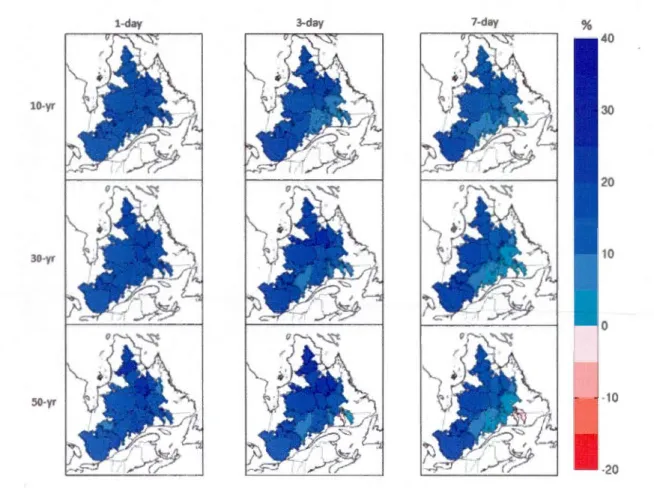
Figure 7 shows ensemble-averaged projected changes to 10-, 30- and 50-yr return levels of 1-,
3- and 7-day precipitation extremes for the future 2041-70 period with respect to the current
1971-2000 period. An increase in return levels in future climate is projected for nearly ail
watersheds, with relatively smaller (positive/negative) changes for sorne of the south-eastemmost watersheds. One- and 3-day return levels are associated with larger increases
compared to 7-day cases. Average change for ali watersheds, return periods and precipitation durations is of the order of 13%, with minimum changes in the 5 to 9% range for the south-eastern watersheds ROM, NAT, CHU and MOI, while maximum changes of the order of 16 to 18% is noted for the northern watersheds (ARN, BAL, FEU, PYR and MEL).
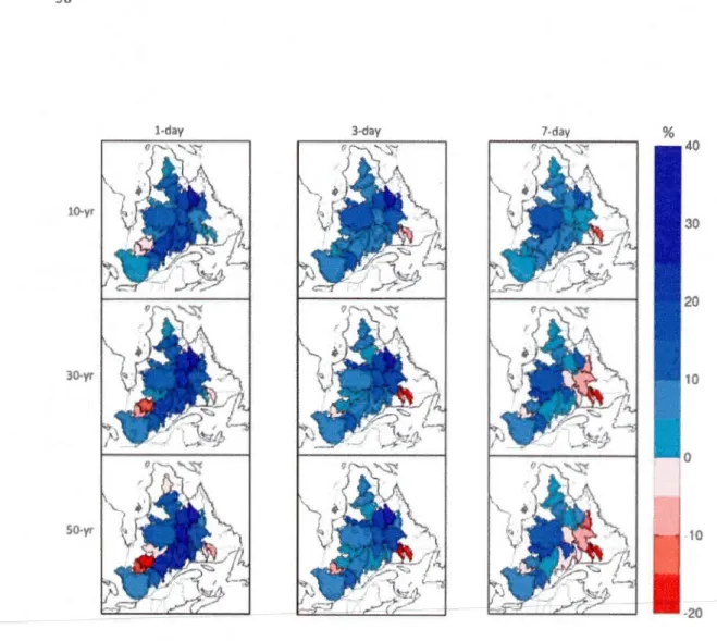
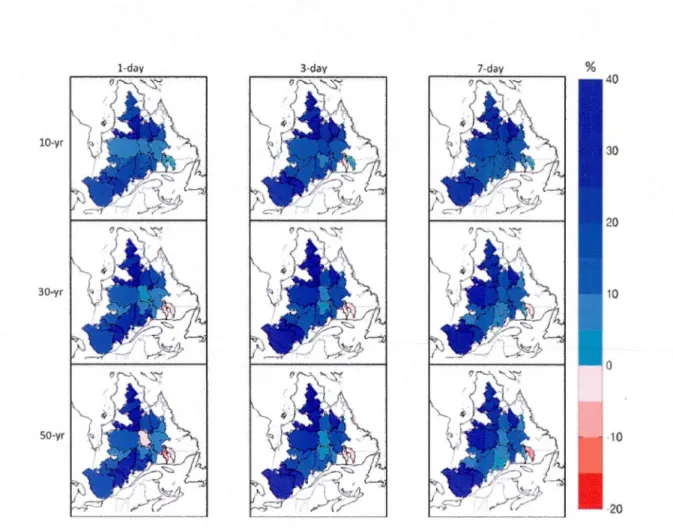
Figures 8 and 9 show CRCM projected changes, when driven by CCSM and CGCM3,
respectively. While the mean changes for ali watersheds lie in the 7% range for CRCM_CCSM, it is around 18% for CRCM_CGCM3. Nevertheless, for both, highest increases in return values are found for short-duration precipitation extremes compared to
longer duration extremes. Wh ile CRCM _ CCSM suggests decreases in return values for the south-eastern watersheds, it is not as widespread for CRCM _ CGCM3. The largest increases are found for the three northernmost watersheds, ARN, FEU and MEL with CRCM_CGCM3 for most of the return levels presented in Fig. 9, while it varies with the duration of
precipitation for CRCM _ CCSM. Thus, though the climate change signal appears to be consistent for most of the watersheds (with the exception of sorne eastern and south-western watersheds), important differences in magnitude can be noted between CRCM_CGCM3 and CRCM _ CCSM projections. Similar to the case of CRCM, noticeable difference is found in
the magnitude of projections for the two RCM3 simulations with average projected increase
of9% for RCM3_CGCM3 and 16% for RCM3_GFDL. The above comparison highlights the
need to use severa! AOGCMs at the boundaries to assess the uncertainty associated with the driving AOGCM.
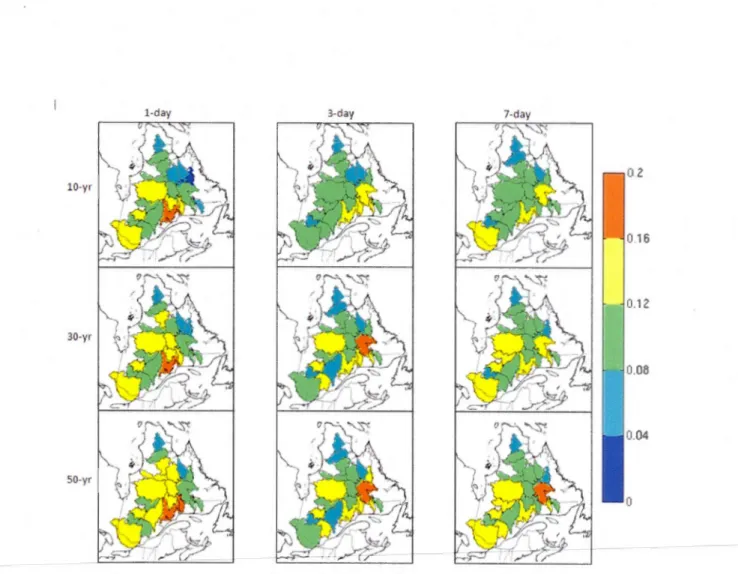
Figure 10 shows the CV (defined in the methodology section) associated with
projected changes to regional return levels for the multi-RCM ensemble. Coefficient of
variation is a useful measure in associating a leve! of confidence with projected changes for
the studied watersheds. The value of CV for projected changes to
Q(l,lû)
is Jess than 1.0 for ail watersheds, suggesting relatively high confidence in the projections for this return leve!for ail watersheds. In ail cases, larger CVs are noted for eastern watersheds (CHU, GEO,
MOI, NAT and ROM), particularly for higher return periods and precipitation durations,
suggesting low leve! of confidence in the projections for these watersheds.
The statistical significance ofprojected changes to single- and multi-day precipitation
extremes from current to future climate is assessed at 5 and 10% significance levels (see Figs.
11 and 12, respectively) using the nonparametric vector bootstrap approach described in the
methodology section. These figures show the number of RCM_AOGCM pairs that suggest statistically significant changes. These results are also summarized in Table 3 for each return period and precipitation duration combination. Majority of the 8 RCM_AOGCM pairs
suggest significant increases in 10-yr return levels of single- and multi-day extremes. The
number of RCM_AOGCM pairs that suggest significant changes is generally limited to 3-5 range for the south-eastern watersheds. With increasing return period, a drop in the number
of pairs that suggest significant changes is obvious in Figs. 11 and 12. Clearly, more number of RCM_AOGCM pairs suggests significant changes at 10% significance leve! for ail cases
shown in these figure . It should be noted that negative changes to selected return levels are
not found statistically significant for any of the watershed.
Finally, it is important to mention that projected changes to precipitation extremes were studied earlier by Mladjic et al. (2011) and Mailhot et al. (2012) for large Canadian climatic regions. Though the results of the present study agree in general with th ose of the