Retrieving spectra from a moving imaging Fourier transform spectrometer

(1)

RETRIEVING SPECTRA FROM A MOVING IMAGING

FOURIER TRANSFORM SPECTROMETER

AHMED MAHGOUB

Doctorat en génie électrique

Québec, Canada

(2)

(3)

Résumé

Afin d’obtenir un spectre de haute résolution avec un spectromètre-imageur par transformation de Fourier (IFTS), il est nécessaire que la scène demeure statique pendant l’acquisition. Dans de nombreux cas, cette hypothèse ne peut pas être respecter simplement à cause de la présente d’un mouvement relatif entre la scène et l’instrument pendant l’acquisition. À cause de ce mouvement relatif, les échantillons obtenus à un pixel capturent différentes régions de la scène observée. Dans le meilleurs des cas, le spectre obtenu de ces échantillons sera peu précis et aura une faible résolution.

Après une brève description des IFTS, nous présentons des algorithmes de d’estimation du mouvement pour recaler les trames des cubes de données acquises avec un IFTS, et desquelles il sera ensuite possible d’obtenir des spectres avec une précision et une résolution élevées. Nous utilisons des algorithmes d’estimation du mouvement qui sont robustes aux variations d’illumination, ce qui les rend appropriés pour traiter des interferogrammes. Deux scénarios sont étudiés. Pour le premier, nous observons un mouvement relatif unique entre la scène qui est imagée et l’instrument. Pour le second, plusieurs cibles d’intérêts se déplacent dans des directions différentes à l’intérieur de la scène imagée.

Après le recalage des trames, nous devons ensuite résoudre un nouveau problème lié à la correction de l’effet hors-axe. Les échantillons qui sont associés à un interférogramme ont été acquis par différents pixels du senseur et leurs paramètres hors-axe sont donc différents. Nous proposons un algorithme de rééchantillonnage qui tient compte de la variation des paramètres de l’effet hors-axe.

Finalement, la calibration des données obtenues avec un IFTS lorsque la scène imagée varie dans le temps est traitée dans la dernière partie de la thèse. Nous y proposons un algorithme de calibration apropriée des trames, qui précède le recalage des trames et la correction de l’effet hors-axe. Cette chaine de traitement nous permet d’obtenir des spectres avec une résolution élevée.

Les algorithmes proposés ont été testés sur des données expérimentales et d’autres provenant d’un simulateur. La comparaison des résultats obtenus avec la réalité-terrain démontre la valeur de nos algorithmes: nous pouvons obtenir des spectres avec une résolution comparable

(4)

à celle qui peut être obtenue lorsqu’il n’y aucun mouvement entre l’instrument (IFTS) et la scène qui est imagée.

(5)

Abstract

To obtain a useful or high resolution spectrum from an Imaging Fourier Transform Spectrome-ter (IFTS), the scene must be stationary for the duration of the scan. This condition is hard to achieve in many cases due to the relative motion between the instrument and the scene during the scan. This relative motion results in multiple data samples at a given pixel being taken from different sub-areas of the scene, and from which (at best) spectra with low accuracy and resolution can be computed.

After a review of IFTS, we present motion estimation algorithms to register the frames of data cubes acquired with a moving IFTS, and from which high accuracy and resolution spectra can be retrieved. We use motion estimation algorithms robust to illumination variations, which are suitable for interferograms. Two scenarios are examined. In the first, there is a global motion between the IFTS and the target. In the second, there are multiple targets moving in different directions in the field of view of the IFTS.

After motion compensation, we face an off-axis correction problem. The samples placed on the motion corrected optical path difference (OPD) are coming from different spatial locations of the sensor. As a consequence, each sample does not have the same off-axis distortion. We propose a resampling algorithm to address this issue.

Finally the calibration problem in the case of moving IFTS is addressed in the last part of the thesis. A calibration algorithm suitable for data cube of moving IFTS is proposed and discussed. We then register the frames and perform the off-axis correction to obtain high resolution spectra.

To verify our results, we apply the algorithms on simulated and experimental data. The comparison between the results with the ground-truth shows promising performance. We obtain spectra with resolution similar to the ground truth spectra (i.e., with data acquired when the IFTS and the scene are stationary).

(6)

List of Figures

2.1 FTS. . . 6

2.2 Effect of OPD length on spectral resolution. . . 8

2.3 Off-axis angle and its effect on the output spectrum. . . 9

2.4 Hyper spectral image/data cube. . . 10

2.5 Blackbodies at different temperatures. . . 11

2.6 Spectra of toluene before and after calibration. . . 13

2.7 IFTS frame before and after calibration. . . 13

2.8 The layout schematic and an output frame from the simulator. . . 14

2.9 Scenario for a gas in absorption or transmission mode. . . 15

2.10 Simulated CO₂ in absorption mode. . . 16

2.11 Experimental setup for SpIOMM. . . 17

2.12 Frequency response of filters. . . 18

3.1 Problem with a single moving target. . . 20

3.2 Non stationary targets before and after motion correction. . . 20

3.3 Monochromatic off-axis correction. . . 22

3.4 Setup for IFTS scanning a target in NIR band. . . 30

3.5 Motion vectors for both methods and the error generated from each method. . . . 31

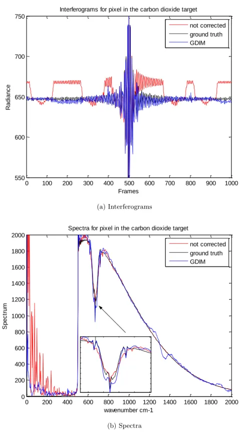
3.6 Interferograms for carbon dioxide at NIR. . . 32

3.7 Spectra for carbon dioxide at NIR. . . 33

(8)

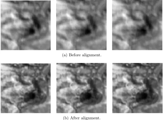
3.9 Frames at wave numbers 6216, 6247, and 6366 cm-1 before (up), and after (down)

alignment. In b), the elliptical shape of CO2 is apparent. . . 35

3.10 The simulated targets. . . 36

3.11 Motion vectors for carbon dioxide. . . 37

3.12 Motion vectors for water vapor. . . 38

3.13 Error in the motion vectors. . . 38

3.14 Interferograms and spectra for the water vapor before and after motion correction. 40 3.15 Interferograms and spectra for the carbon dioxide before and after motion correction. 41 3.16 Resolution target and filters. . . 42

3.17 Resolution target and motion vectors. . . 42

3.18 Interferograms after motion correction for the red filter. . . 43

3.19 Spectra after motion correction for the red filter. . . 44

3.20 Spectra generated from the opaque filter. . . 44

3.21 The simulated targets. (Left) is the is the green LED light and (right) is the hole. 45 3.22 Motion vectors for GDIM. . . 46

3.23 Interferograms and spectra for the green LED before and after motion correction. . 47

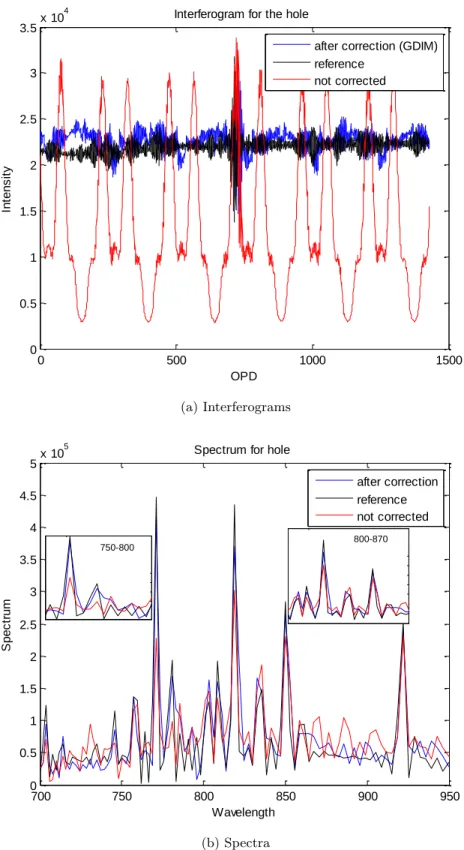
3.24 Interferograms and spectra for the hole before and after motion correction. . . 48

4.1 Monochromatic off-axis correction. . . 53

4.2 Off-axis correction algorithm. . . 54

4.3 Simulated wave-number map. . . 55

4.4 Spectrum of water vapour after using non-uniform off-axis correction and the errors generated from the spectral shift off-axis correction. . . 55

4.5 Spectra from non-uniform off-axis correction and LMSE-spectral shift off-axis cor-rection. . . 56

4.6 Off-axis map before and after increasing resolution. . . 57

4.7 Spectra after off-axis correction. . . 58

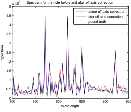
4.8 Spectra of the hole before and after off-axis correction. . . 60

5.1 ABB IFTS gain function used for un-calibrating the simulator. . . 64

5.2 ABB IFTS offset function used for un-calibrating the simulator. . . 65

5.3 Gain and offset functions used to calibrate the spectrum. . . 65

5.4 Calibrated interferogram and spectrum compared to the references. . . 67

5.5 Stationary cube before and after calibration normalized to unity. . . 67

5.6 Interferogram of a pixel that views in alternance the background and the target during a scan. . . 69

5.7 Ratio map between the dc levels in raw interferograms. . . 71

5.8 The raw interferogram and the ratio function. . . 72

5.9 The raw and calibrated spectra. . . 73

5.10 The calibrated interferogram before and after applying the ratio function. . . 73

5.11 Non-stationary cube before and after calibration. . . 74

5.12 The complete procedure for calibration, motion, and off-axis correction. . . 75

5.13 Motion vectors for the carbon dioxide target using GDIM. . . 75

5.14 Motion vectors for the water vapor target using GDIM. . . 76

5.15 Error in motion vectors for the carbon dioxide target using GDIM. . . 76

5.16 Error in motion vectors for the water vapour target using GDIM. . . 77

5.17 Interferogram and spectrum for calibrated carbon dioxide before and after motion correction. . . 78

(9)

5.18 Calibrated carbon dioxide before and after off-axis correction. . . 79

5.19 Interferogram and spectrum for calibrated water vapour before and after motion correction. . . 79

5.20 Calibrated water vapor spectrum before and after motion correction for the sensor operating band. . . 80

5.21 Calibrated water vapor spectrum before and after off-axis correction. . . 80

5.22 Toluene target moving, the frames show frame 1000 to 8000 in a step of 1000. . . . 81

5.23 Spatial locations for the background and target interferograms. . . 83

5.24 Interferograms for a background pixel before and after calibration. . . 84

5.25 Interferograms for a target pixel before and after calibration. . . 84

5.26 Interferograms contains samples from background and target before calibration, and the ratio function. . . 85

5.27 Interferogram for a pixel contains samples from background and target after cali-bration and a zoom window around the ZPD. . . 85

5.28 ABB non-stationary cube before (the right column) and after calibration (in the left column). . . 86

5.29 Pixel motion vectors for raw and calibrated toluene. . . 87

5.30 Sub-pixel motion vectors for raw and calibrated toluene. . . 88

5.31 Sub-pixel motion vectors for raw and calibrated toluene around the ZPD. . . 88

5.32 The ZPD frame and the examined pixels. . . 89

5.33 Pixel 21,52 before and after calibration and motion correction. . . 90

5.34 Pixel 52,51 before and after calibration and motion correction. . . 91

A.1 Scenario for successive gases in absorption or transmission mode. . . 103

A.2 Simulated CO2 and H2O in absorption mode. . . 104

A.3 Line strength at 296K of some gases simulated with Hitran. . . 105

A.4 Output frames from the simulator in the LWIR. . . 108

A.5 Scenario for an IFTS in the NIR band. . . 109

A.6 Reflection of earth’s surface (upper left), radiance of sun after transmitted through CO2 column (upper right), signal received by IFTS (down left), and the column of the CO2 (down right). . . 109

A.7 Output frames from the simulator in the NIR. . . 110

B.1 Motion vectors evaluation through 4 iterations. Iteration 1 (upper left corner), iteration 2 (upper right corner), iteration 3 (lower left corner), and iteration 4 (lower right corner). Last row is a zoom on the motion vectors after iteration 1 (left) and 4 (right). . . 112

B.2 The evolution of the multiplier factor through the iteration of the GDIM. Each iteration the multiplier factor is divided from the test frame. Iteration 1 (upper left corner), iteration 2 (upper right corner), iteration 3 (lower left corner), and iteration 4 (lower right corner). . . 113

B.3 The k and k+1 frames, where the red color indicates the vertical direction (x), and the yellow color indicates the horizontal direction (y). The 10 colored pixels are used to compute the average brightness value. . . 114

(10)

(11)

Acknowledgments

I would like to express my special appreciation and thanks to my supervisor Professor André Zaccarin. You have been a tremendous mentor for me. I appreciated your encouragement, guidance, and support. I feel honored to have been given the opportunity to contribute to research under your supervision.

My appreciation also goes to my co-supervisor Raphaël Desbiens. Your advice on both research as well as on my career have been priceless. You directed my thesis to the industry domain which helped me to link research to industry. I also thank you for all what you did to help me settle with my family in Quebec city.

I would like to thank Prof. Drissen and the Groupe de recherche en astrophysique, who gave us access to their instrument to complete this work. Thanks for the training and support to use the instrument and your data.

Also, I would like to pay my humble respects to my family, especially my parents: My mother (God bless her), who did not have the chance to see me in this day, my father who waited a long time for this day. Your prayer for me was what sustained me thus far.

A special thanks to my beloved wife Amira. Words can not express how grateful I am to all your sacrifice and support for me since our mariage. You give me love, guidance, self confidence as well as sharing ideas in the research with me. I will never forget that you were always my support in the moments when there was no one to answer my queries.

(12)

(13)

Chapter 1

Introduction

This thesis presents a research project that was realized at the Laboratoire de Vision et systèmes Numériques (LVSN) at l’Université Laval. The subject of this work was initially defined in a research collaboration between Prof. Zaccarin and ABB lnc. It was partly funded by the Natural Sciences and Engineering Research Council of Canada and ABB Inc. Most of the experimental work was made possible by the collaboration of Prof Drissen, from the Groupe de recherche en astrophysique, who gave us access to SpIOMM, an imaging Fourier transform spectrometer.

1.1 Applications of Imaging Fourier Transform Spectrometers

Imaging Fourier Transform Spectrometers (IFTS) are important systems for remote sensing imaging applications because of their ability to provide, simultaneously, both high spatial and spectral resolution images of a scene. The spectral data obtained from a high resolution imaging FTS is often classified as "hyper spectral".

The idea of IFTS was first proposed in 1972 [37]. However, it is only in the 1990s that we had the first IFTS that produced valuable scientific results [32]. Nowadays, IFTS has proved its competency in many applications because of its ability to provide rapid and non-destructive analysis both spectrally and spatially.

In the field of biomedical imaging and sensing, microspectroscopy is used for cancer pathology and tumor diagnosis to obtain more information about the composition of the tumor tissue [4, 5, 7, 45]. In environmental domain, IFTS are used for remote detection of gases and liquids, hazardous vapors, and monitoring of the ozone layer [51, 17, 20]. They are also used by the military for remote detection of camouflaged vehicles, analysis of aircrafts exhaust, and standoff chemical detection [1, 43, 40]. IFTS are also particularly suited for applications in astronomy because of their high sensitivity to light. They are used, among others, for studying the statistics and physics of galaxy and the early stages of star formation [42, 48, 33].

(14)

1.2 Motivations

An IFTS produces a data cube where the x and y axis are the spatial coordinates of the scene, and the interferogram samples are found along the z axis. The IFTS captures one interferogram for each of its sensor elements (pixels). The Fourier transform of each interferogram generates an estimate of the radiometric spectrum, within the sensor band, radiated by the scene element imaged by that pixel. For maximum spectral accuracy and resolution, each interferogram sample must come from the same location in the scene. This means that the scene being imaged must be stationary for the duration of the scan, which may last from less than a second to many hours depending on the application. This condition is hard to achieve in many cases due to the relative motion between the instrument and the scene, or simply because of the nature of the scene being imaged. This relative motion or motion in the scene will, at best, reduce the spectral resolution of the data, and at worst make the data unusable.

When there is relative motion between the scene and the instrument, or within the scene, we need to build an interferogram for each scene element from the interferogram samples of the data cube. So, if the instrument underwent a motion in a certain direction and we knew the parameters of that motion, we would only need to shift the image planes in the direction opposite to that motion. In space-borne and airborne FTS imagers, motion compensation is done using opto-mechanical means to keep the sensor pointing on the same ground area for the duration of the scan. We propose instead to perform motion compensation a posteriori, using the data information. This is simpler as it requires no hardware and can be used to compensate for non-predictable motion where pointing mechanisms do not work.

Motion compensation in the image plane of the interferograms is conceptually interesting but not as straightforward as it may sound. Most motion compensation techniques, like the one developed for video compression, assumes that the signals they want to align have constant intensity. An interferogram signal is a modulated signal and is not constant. Interferogram samples, besides being measurements of a specific scene element, have properties that directly tie them to a pixel on the sensor from which they were acquired. First, the sampling interval of the interferogram is typically not uniform throughout the sensor. Second, the calibration parameters are also not uniform throughout the sensor (calibration is needed to convert a sensor reading from a relative to an absolute scale). Registration of the image planes of a data cube acquired by an IFTS needs to take into account these two properties in order to generate interferograms from which electromagnetic spectral information can be extracted accurately and with high resolution.

1.3 Objectives and Major Contributions

Our objective is to develop algorithms to process data acquired by an IFTS (without opto-mechanical pointing mechanisms) when there is a relative motion between the scene and the

(15)

instrument or within the scene, in order to reduce the impact of this motion on the spectral accuracy and resolution of the acquired data.

We can summarize the contributions in this thesis as :

- Development of suitable motion estimation algorithms to align the frames of a data cube acquired by an IFTS when there is relative motion between the scene and the instrument or within the scene. With these algorithms, we generate data cubes where each interferogram has only samples coming from the same scene location.

- Development of an algorithm that takes into account the spatially varying sampling interval of an instrument and resamples the interferograms after motion compensation so that each interferogram is sampled uniformly.

- Development of an algorithm to calibrate the data cube acquired by an IFTS while preserving the information required for motion compensation of that data.

1.4 Thesis Organization

Chapter 1 summarizes the motivation, the objectives and the main contributions of this re-search. Chapter 2 presents an overview of FTS and IFTS including the background information that will be used later in the thesis. The simulated and experimentally acquired data cubes that are used for this research are described in Chapter 2.

A description of the problem coming with data cubes acquired from a moving IFTS is given in Chapter 3. We survey different image registration techniques appropriate for our problem and describe the algorithms we have developed for registering the frames of the data cubes. Results obtained with these algorithms on simulated and experimental data are given. In Chapter 4, we present the concept of off-axis distortion, and its spatial dependance (which is the result of the spatially varying sampling interval of an IFTS), and we propose an algorithm that takes into account and corrects the mixed off-axis distortion of a motion compensated interferogram. Results obtained on simulated and experimental data are given.

In Chapter 5, we discuss the impact of calibration on our algorithms. We discuss the difference between calibrating a data cube acquired from a fixed IFTS and the challenge of calibrating data cube acquired from a moving IFTS. We present an algorithm for calibrating a data cube acquired with a moving IFTS and give results on simulated and experimental data. Motion compensation, mixed off-axis distortion and calibration are integrated and used to process data cubes.

(16)

(17)

Chapter 2

Imaging Fourier Transform

Spectrometer and Data Cube

Acquisition

This chapter presents a general review of the basics of FTS and IFTS instruments. The review is not exhaustive but concentrates on the needed information that is most relevant to our project. In the second part of the chapter, we describe the IFTS data cubes both simulated and experimentally used in this thesis. The simulated data is generated from a simulator designed for the purpose of this research. The experimental data was acquired from an IFTS prototype at ABB Bomem and an IFTS for astronomy.

2.1 Fourier Transform Spectrometer

A Fourier Transform Spectrometer (FTS) captures the electromagnetic spectrum of a source by measuring the temporal coherence of a radiative source. A beam of light is split into two beams and reflected off two mirrors. At least one of the mirrors is moving to change the optical path difference between the two beams. The reflected beams are then brought together and the amplitude of the interference pattern is measured. An interferogram is measured by sampling the interference pattern for different optical path differences. The Fourier Transform of this interferogram returns the spectrum of the input source. Figure 2.1 shows a Michelson interferometer that is considered as the heart of the FTS. Given a monochromatic source A(σ0), where σ0 is the wave-number (reciprocal of wavelength), the intensity of the interferogram, as a function of the optical path difference (OPD) x between the two beams, is given by

It(x) = 2A(σ0)[1 + cos(2πσ0x)] (2.1)

(18)

Source M o vin g m irr o r Fixed mirror Beam split ter Detector -OPD ZPD +OPD Figure 2.1: FTS.

The zero path difference (ZPD) is the location where the optical path difference is zero, and is the point where the interferogram is maximum. This occurs when both mirrors are equally apart from the beam splitter. At this point the size of the interference pattern is infinite, and the central fringe occupies the entire image plane.

2.1.1 From Monochromatic to Polychromatic

When the source contains more than one frequency, the detector detects a superposition of such cosines. The monochromatic light A(σ₀) will be replaced by a polychromatic light, which has a spectrum of B(σ). The equation can be expressed as

It(x) = 2

Z ∞

0

B(σ)[1 + cos(2πσx)]dσ (2.2)

that in turn can be arranged to

It(x) = 2 Z ∞ 0 B(σ)dσ + 2 Z ∞ 0 B(σ)cos(2πσx)dσ (2.3) = I(0) + I(x)

where I(0) is a constant value and I(x) is the part of the interferogram, which after a Fourier transform, gives the spectrum.

The interferogram and its spectrum are related by a cosine transform, which is suitable for an ideal interferogram that is symmetric about the ZPD. Hence we have the following transform

(19)

pair I(x) = Z ∞ −∞ B(σ)ej2πσxdσ = F−1{B(σ)} B(σ) = Z ∞ −∞ I(x)e−j2πσxdx (2.4) = F {I(x)} I(x) ⇐⇒ B(σ)

where, F−1{} is the inverse Fourier transform operator and F {} is the Fourier transform operator, and the ⇐⇒ is the Fourier transform conversion [24].

2.1.2 Spectral Resolution

Spectral resolution describes the ability of a sensor to define fine wave-number intervals. The output spectrum is characterized by the maximum wave-number that depends on the sampling rate of the interferogram, and its resolution that depends on the length of the OPD. To have a high resolution spectrum, the OPD must be extended to high values. For a given maximum OPD, the unapodised spectral resolution is given by

δσ = 1

2 × OP Dmax· (2.5)

Having an OPD extending to infinity results in a spectrum with an infinite resolution. This is obviously impossible to obtain because the moving mirror can only travel a finite distance. The interferogram is truncated as the mirror reaches the minimum or the maximum OPD. Truncating the interferogram is equivalent to multiplying the infinite length interferogram with a boxcar function.

Instrument Line Shape Function

The truncated interferogram can be written as

IL(x) = Π2L(x)I(x) (2.6)

where, I(x) is interferogram before truncation, Π2Lis the boxcar function that equals one when |x| ≤ L and zero otherwise, L is the OPD path length, and finally I_L is the interferogram after truncation.

Taking the Fourier transform of the previous equation gives

AL(σ) = WL(σ) ∗ A(σ) (2.7)

where W_L(σ) = 2Lsinc(2πσL) and is the transform of the boxcar function, and ∗ is the convolution operator. Convolution of the the spectrum A(σ) with W_L(σ) lowers the resolution of the output spectrum AL(σ) [24].

(20)

To show the relation between the OPD, ILS and the spectral resolution, we simulated two spectra for CO₂. We changed the length of the OPD in two similar scans. The first spectrum has a relatively short OPD (1000 samples) with a spectral resolution of 4 cm−1, while the second spectrum has an OPD four times longer (4000 samples) to give a spectral resolution of 1 cm−1. The sensor operating band is between 500 cm−1 to 2000 cm−1, with a sampling rate twice the highest wave number. Figure 2.2 shows the effect of changing the length of OPD on the spectral resolution. We can clearly see that the spectrum obtained with the

500 550 600 650 700 750 800 45 50 55 60 65 70 75 80 85 90 95 100 wave number s p e c tr u m

Spectrum of CO2 with 1000 samples

500 550 600 650 700 750 800 45 50 55 60 65 70 75 80 85 90 95 100 wave number s p e c tr u m

Spectrum of CO2 with 4000 samples

Figure 2.2: Effect of OPD length on spectral resolution.

interferogram with the longer OPD has a higher resolution than the spectrum generated with the interferogram with shorter OPD. We use this relation to setup the resolution of the simulated output data cubes used in the thesis.

2.1.3 Off-axis Effect

Real light sources are never just points, but they are extended sources with finite sizes. So, when light rays enter the interferometer, they make different angles with respect to the optical axis. An off-axis light ray is modulated at a lower frequency than a light ray on the optical axis when we move the mirror of the interferometer. This implies that the interferogram scale is compressed for pixels that are off-axis (i.e., the interferograms are not sampled at the same interval as a function of the location of the pixels on the sensor). This is the off-axis effect. The scale compression is a function of the angle between the off-axis and on-axis pixel. We use the small angle approximation to calculate the off-axis effect for the simulated data in the thesis. We use cos(θ) ≈ (1 −θ₂2), where θ is the angle between the incoming ray and the optical axis, and cos(θ) is the off-axis effect. Assume that the radius of the circle for a circular

(21)

radiation source is r, and its focal length is f , then r ≈ f θ ,and cos(θ) ≈ (1 − r2

2f2). According

to the equation of the interferogram, the intensity at a point source not on the optical axis will be

I(x) = 2

Z ∞

0

A(σ)cos(2πσxcos(θ))dσ (2.8)

This intensity will be modified for a circular source and will depend on the off-axis angle as follows I(x) = 2 Z 2π 0 Z θmax 0 Z ∞ 0 A(σ)cos(2πσxcos(θ))dσsinθdθdφ (2.9)

The off-axis effect causes the interferograms to be sampled at slightly shorter OPD, therefore, affecting the interferogram in the space domain as well as affecting the spectrum in the spectral domain. The spectra appear to be expanded to slightly lower wave numbers, causing them to have different spectral sampling intervals. At the centre pixel the off-axis has a small impact, whereas the greatest effect is experienced by the corner pixel elements. We define σ0 as the wave-number of the central pixel with the minimum off-axis effect, and σ is the wave-number for any other pixel. They are related by the cosine of the off-axis angle θ as _σσ

0 = cos(θ).

Figure 2.3a shows the off-axis angle. Figure 2.3b shows the spectrum of a monochromatic

(a) Off-axis angle

14500 1460 1470 1480 1490 1500 1510 1520 1530 1540 1550 50 100 150 200 250 300 wave-number cm-1 In te n s it y

spectra of monochromatic signal at 1500cm-1 with maximum off-aixs angle 100mR off-axis (corner pixel) on axis (central pixel)

(b) Off-axis effect

Figure 2.3: Off-axis angle and its effect on the output spectrum.

corner pixel with an off-axis angle of 100mRad, out of a centre pixel with no off-axis effect. The wave number is set to be 1500 cm−1. The off-axis correction algorithm must remap the spectra to their correct wave-number grids.

(22)

2.1.4 Imaging FTS and Hyper Spectral Image/Data Cube

Instead of using a single detector (which is the case of FTS), the imaging FTS uses an array of detectors. They are usually arranged in a rectangular or a square shape. This array of detectors is capable of acquiring high resolution spectral images over a specified area that can be recorded as hyper spectral images. Hyper spectral images are defined as being recorded in many, narrow, contiguous bands to provide information on the major features of the spectral reflectance of a given object. The images can be visualized as a 3-dimensional data set with two spatial and one spectral dimension, and the data set is therefore often referred to as an image cube. Hyper spectral data provide detailed information on the emission and absorption features of the spectral reflectance of a given object. Figure 2.4 illustrates the concept of a hyper spectral data set. It can be seen as a stack of spatial images over different spectral channels or as a stack of spectra arranged in an array of pixels. The upper left cube describes the frames in the time domain. When tracking a single spatial pixel in the axis of time, we will have the interferogram of that pixel. If this cube of data is transformed to the frequency domain where the Fourier transform will be applied to each spatial pixel along the time, it will result in a hyper spectral data cube. Because of the spatial-spatial-spectral dimensional nature of the hyper spectral data sets, they are often referred as image/data cubes. As stated in [47], the data that are extracted from the IFTS is correlated both spatially and spectrally due to the homogeneities of features covered by the surrounding pixels and the overlap of information across the adjacent channels [47, 24, 23].

Spectral channel Interferogram channel Examined pixel

FT

Figure 2.4: Hyper spectral image/data cube.

2.1.5 Calibration

Measurements obtained from a FTS suffer from the effect of the gain and offset factors of the instrument. For this reason, an instrument must be calibrated against some form of

(23)

reference so that measurements can be corrected using this calibration information [38]. The calibration process depends mainly on comparing the spectrum with two reference spectra that are generated from blackbodies. In this section we define the blackbodies and the calibration for IFTS data cubes.

Blackbodies

Blackbodies are bodies that emit or absorb all the radiation. They emit or absorb the maxi-mum amount of radiation possible for a body at a specified temperature. They are a convenient baseline for radiometric calculations, since any thermal source at a specified temperature is constrained to emit less radiation than a blackbody at the same temperature [50]. Figure 2.5 shows blackbody curves at different temperatures.

0 500 1000 1500 2000 2500 3000 3500 4000 0 0.1 0.2 0.3 0.4 0.5 0.6 0.7 wave number cm-1 In te n s it y ( w a tt /m 2 c m -1 s r) BB at 250K BB at 300K BB at 350K BB at 400K BB at 450K

Figure 2.5: Blackbodies at different temperatures.

In 1900, Max Planck derived the theoretical solution that quantifies the blackbody radiation distribution. The Planck function expresses the radiance emission of a blackbody according to its wavelength as

Bλ(T ) = 2hc

2_λ−5

ehc/λKT_{− 1} (2.10)

where h is Plank’s constant, c is the light velocity in m/sec, λ is the wavelength, T is the temperature in Kelvin, and k is Boltzmann’s constant. The previous equation represents the blackbody radiation at a single wavelength. It may be preferred to work with wave number instead of wavelength. Wave number is a unit that can be related to the wavelength as σcm = _100λ1 . The blackbody equation can be written as a function of wave number but the

(24)

energy integrated over both representations must be equal Bσ(T ) = 2hc

2_σ3

ehcσ/KT _{− 1} (2.11)

Calibrating the spectra

The raw data magnitude spectrum C_σ can be modeled as

Cσ = Rσ(Lσ+ Lσ0) (2.12)

where C_σ is the observed raw spectrum from the scene, L_σ is the incident radiance, R_σ is the spectral responsivity of the instrument, and L_σ0 is the instrument emission or the offset (that can be defined as the radiance which, if introduced at the input of the instrument, would give the same contribution as the actual emission from various parts of the optical train).

The calibration is usually done with the help of known radiance sources such as blackbodies. We use two blackbodies at cold and hot temperatures for calibration. The linear relationship written for both the hot and cold blackbody observed raw spectrum

Cc= Rσ(Bc+ Lσ0) Ch = Rσ(Bh+ Lσ0)

can be solved to yield

Rσ = (Ch− Cc) Bh− Bc Lσ0 = Ch Rσ − Bh (2.13) = Cc Rσ − Bc

where B_h and Bcare the Planck blackbodies radiances for the hot and cold blackbodies, while Ch and Ccare the radiance from the known sources (physical blackbodies). From the previous equations and solving for a science target spectrum yields the basic calibration relationships

Lσ = Cσ Rσ

− L_σ0 (2.14)

We apply the calibration equation on the spectra obtained from an IFTS data cube scanned at ABB Bomem. We scanned two blackbodies at cold and hot temperature for the calibration purpose. The IFTS scans a transparent container with Toluene gas. Figure 2.6 shows the spectra of toluene before (i.e., C_σ) and after (i.e., L_σ) calibration. Figure 2.7 shows a frame before and after calibrating all the spectra of the data cube each at its spatial location. We can see the effect of calibration that manages to eliminate the black circles at the center of the frame. This is important for the motion estimation algorithm that is used to align the frames generated from a moving IFTS instrument.

(25)

950 1000 1050 1100 1150 1200 1250 1300 1350 0 0.5 1 1.5 2 2.5 3 3.5 4 4.5 5x 10 4 Wave-number S p e c tr u m

Spectra before and after calibration

Before calibration After calibration

Figure 2.6: Spectra of toluene before and after calibration.

Frame before calibration Frame after calibration

(26)

2.2 IFTS Data Cube Acquisition

In this section we discuss the methods to acquire IFTS data cubes that will be used in the thesis. We use a simulator to generate data in the long wave infra red (LWIR) and near infra red (NIR) bands. Also, we use experimental data cubes generated from IFTS instruments at ABB Bomem and Laval University. We generate both stationary and moving data cubes. Moving data cubes can have a relative global motion between the instrument and the targets, or more than one target moving in the scanned scene of the IFTS.

2.2.1 Simulated Data

A simulator has been designed in order to generate data cubes with varying characteristics. With the simulator, we can simulate target motion with different parameters for the IFTS (several gas spectra, integration area for the detectors, etc.)

The output of the simulator represents an array of detectors of an infrared camera. Each pixel in this camera gives a value related to the integration of the incident light from the IFTS on it. The dimension of this array can be varied. A schematic for the output layout of a frame is shown in Figure 2.8a. The integration in the detector is implemented by dividing each pixel to 100 sub-pixels then integrating their values. These sub-pixels can be adjusted afterward to put in consideration the area occupied by the electronics in the infrared camera (fill ratio). The red circles show the loci where the pixels have the same off-axis effect. For simplicity in some of the output generated cubes, the off-axis may be calculated one time only for each pixel location and its value is assigned to all the sub-pixels related to this pixel. An output frame representing two different targets is shown in Figure 2.8b. The red arrows show the direction of motion for the targets through the frames.

(a) Simulator output layout schematic (b) An output frame

(27)

A Target in Absorption or Transmission Mode in LWIR Band

In the scenario shown in Figure 2.9, a plume of gas in absorption or transmission mode is moving in front of a background. The background can be an instrumental blackbody or can be the Earth’s surface or the Sun in the case of scanning the atmosphere. An example for this scenario in the absorption mode is a plume of carbon dioxide gas at a temperature less than the temperature of the background so the carbon dioxide absorbs the radiation. If the temperature of the carbon dioxide is higher than the temperature of the background, the carbon dioxide will be in the emission mode. We use this scenario for generating the data through out the thesis. The output radiance can be calculated as:

Ttarget

Ltarget

Lin Lout

Figure 2.9: Scenario for a gas in absorption or transmission mode.

Lout = LinTtarget+ Ltarget(1 − Ttarget) (2.15) where Ttarget is the target transmittance and depends on target temperature, length of the path in the target, target concentration, etc.; and L_inis the input radiance, L_out is the output radiance, and Ltarget is the blackbody radiance at the target temperature.

An output radiance for this scenario is shown in Figure 2.10 where carbon dioxide is simulated at a height of 6km above the Earth’s surface at a temperature of 250K in front of a blackbody at temperature 300K, representing the Earth. We can see the absorption lines of the carbon dioxide. This setup can be extended to scanning two or more successive gases absorbing or transmitting as shown in appendix A.

A Target in the NIR Band

Working in the NIR range, we can assume that there is negligible emission from Earth’s surface, so the radiation from the Sun that is transmitted through the column of the gas is reflected on Earth’s surface toward the IFTS. The emission from the Sun in this spectral band is simulated from the spectral radiance of a blackbody at temperature 6000K according to Planck’s equation. The reflectance of Earth’s surface is simulated from NASA database [41] at this range and is normalized to 0.4 as a maximum reflection coefficient. The transmittance of CO2 is computed from Hitran spectroscopic parameters. We use this setup to generate IFTS data cubes in the NIR band. More information about the setup is found in appendix A.

(28)

500 1000 1500 2000 0 0.02 0.04 0.06 0.08 0.1 0.12 0.14 0.16 wave number S p e c tr u m

Absorption lines for CO2

Figure 2.10: Simulated CO₂ in absorption mode.

2.2.2 Experimental Data

Two sources of experimental data cubes are used in this thesis: from an instrument of ABB Bomem and from SpIOMM (Spectrometre Imageur de l’Observatoire du Mont-Megantic) at Laval University.

ABB Bomem Experimental Data

An IFTS prototype working in the infrared range is used to acquire experimental data cubes at ABB Bomem. A blackbody radiates behind the target and the transmitted radiation is captured by a 16 bit thermal camera. The data cube contains nearly 8000 frames with dimension 64*64. The system is guided by a sinusoidal laser beam at frequency of 15,798 Hz. The detector IR signals are sampled at equal spaced intervals, so we can eliminate the sampling position error.

SpIOMM Experimental Data

SpIOMM is an imaging FTS for astronomy that was assembled in 2004 at Laval University. It was developed in collaboration with ABB Bomem, INO (Institut national d’optique), and the Canadian Space Agency. It is designed to be attached to a telescope for space and galaxy observation. There are successful observing runs using the SpIOMM at the observatoire du Mont Mégantic in southern Québec[16, 15, 11, 12]. SpIOMM operates in the visible range (350-900nm) with a circular field of view of 12 arcminutes in diameter. Its detector is blue-sensitive, liquid nitrogen-cooled with spatial resolution of 1340 x1300 pixels. The physics of

(29)

SpIOMM depends on the classical Michelson interferometer with two outputs ports. One port is only used and the interferogram is recorded by individual images at each OPD step. The interferometer is controlled with a laser-based servo system that is programmed to control the position of the mirror. The interferogram is sampled at a step size determined by the Nyquist criteria. The readout time of the detector is around 5 seconds. Figure 2.11 shows images taken in the laboratory at Laval University. The left image shows the SpIOMM instrument with the camera. The right image shows the set-up used to control the motion of the targets. A metal

(a) SpIOMM instrument (b) Robots to move targets

Figure 2.11: Experimental setup for SpIOMM.

frame is supporting the SpIOMM in the vertical direction. To access the field of view, we designed a wood base with a square hole in the center and installed it on the top of the metal support as shown in the right of Figure 2.11. We combine two lamps to form the light source for the experiment: a wide spectrum argon lamp [2] including several peaks at the range of 700nm to 900nm, and a halogen lamp with a continuous spectrum from 300nm to 900nm. This combination creates a light source with wide continuous background and sharp peaks. We install a resolution target or visible filters in front of the field of view. The light emitted from the lamps is reflected by the ceiling then passed through the filters or the resolution target to reach the camera. Figure 2.12 shows the frequency response of the filters. We use the filters with cut-off frequency at 715nm and 1000nm in our experiments. All the system is covered with black heavy cloth to isolate it from the surrounding light.

(30)

Figure 2.12: Frequency response of filters.

2.3 Conclusion

In this chapter we presensted a fast review for FTS and IFTS technology. We discussed spectral resolution, off-axis distortion and spectral calibration that will be used in this thesis. We end the chapter with data cube acquistion both simulated and experimental.

(31)

Chapter 3

Motion Correction

This chapter defines the problem and the effect of acquiring a data cube from a moving IFTS. As a result of acquiring a hyper-spectral cube from a non stationary IFTS, the output spectra have degraded spectral resolution and accuracy. The chapter covers the concepts of optical flow techniques and classifies them according to the performance under the brightness variation. Applying the optical flow techniques on simulated and experimental data cubes of IFTS is presented.

3.1 Problem Illustration for Motion

This section describes the effect of motion on the output spectra of IFTS. We examine two cases, a global relative motion between the instrument and the target, and the case with more than a target moving in the field of view of the IFTS.

3.1.1 Defining Problem with a Single Moving Target

For a given data cube with no relative motion between the instrument and the scene, the interferogram of each spatial location is constructed from the samples along the OPD axis (scanning axis) of the spectrometer. However, for a cube with a relative motion between the instrument and the scene, the samples of the interferogram are not related to the same spatial location. The interferograms are constructed from samples of different spatial locations according to the relative motion between the instrument and the target. The upper part of Figure 3.1 shows how the samples of the interferogram are constructed in the case of relative motion. Along the selected OPD axis, the samples of the interferogram start at a spatial location corresponding to a target labelled "1". While scanning, the samples of the interferogram are not always related to the target due to the motion. They are related to other spatial location while the locations of the target are indicated by locations "2,3,4". We need to align the frames of the spectrometer in the case of relative global motion to achieve a realigned cube with frames as shown in the lower part of figure 3.1. In the realigned cube,

(32)

the samples of the constructed interferogram are contributed by the spatial locations "1,2,3,4" that are always related to the same target.

Figure 3.1: Problem with a single moving target.

3.1.2 Defining Problem with Multiple Moving Targets

Consider two targets A and E with dimensions one by one pixel as shown in Figure 3.2a. The target located at pixel A is stationary and the other target located at pixel E is moving to pixel location H, K, and L in frames 2, 3, and 4 respectively. Along the OPD axis of pixel A, we find the interferogram samples related to the same pixel location in the next frames. While along the OPD axis of pixel E, the interferogram samples are related to other spatial areas that occupy this place. Our goal is to track the target along the frames, so when we reconstruct the interferogram for pixel E, it contains samples from pixel H in the second frame, pixel K in the third frame, and pixel L in the fourth frame. Tracking target E along the frames gives

A B C H G I F E D J K L A B C H G I F E D J K L A B C H G I F E D J K L A B C H G I F E D J K L OPD OPD

(a) Before correction

A B C H G I F E D J K L A B C H G I F D J K L A B C H G I F D J K L A B C H G I F D J K L OPD OPD . . . (b) After correction

(33)

an interferogram constructed from samples always related to the same target. We need to construct another cube contains interferograms each with samples related to the same spatial location. Figure 3.2b shows the cube after correction.

3.1.3 Effect of Motion on the Interferogram and Spectrum

To examine the effect of motion on the interferogram and the spectrum, we consider a scene that is a background of a blackbody at 300K , and a CO2 target at 250K in absorption mode. This scenario represents a carbon dioxide gas at height of 6 km over the earth’s surface which is scanned in front of the surface of the earth. The target moves from the lower right corner to the upper left one in a step of 0.1pixel/frame. We simulate a grid of the output detectors of 128x128 pixels with 1000 frames. The ZPD is at frame 501. We ignore the noise and shear effect while setting a maximum off-axis angle of 0.04 Rad. The output sample is a 16 bit pixel to simulate the infrared camera. The sensor operating band is between 500-2000 cm−1 wavenumber. The sampling rate is twice the maximum frequency of the input spectrum. We track the interferogram of the pixel located at the border of the CO₂ column of gas. We compare this pixel with another pixel in a stationary cube. Figure 3.3 shows the effect of motion on the interferogram and the spectrum. From the scanned interferogram of the moving target, we recognize that the samples on the OPD are related to the background at the beginning of the scan till the area around the ZPD. The intensity of the background samples is higher than the intensity of the samples of the target because the target is in the absorption mode. Around the ZPD, the samples are related to the CO2, then the samples are related to the background when moving further along the OPD. Most of the information is placed around the ZPD. The far OPD affect mainly the resolution of the spectrum. We can see the errors (i.e low resolution) in the spectrum obtained from the moving target when compared to the spectrum obtained from the non moving target. The goal is to correct for the motion in order to maintain a useful or a high resolution spectrum representing the target.

3.1.4 Motion Compensation

In order to obtain high spectral accuracy, the scene has to be stationary in the field of view of the IFTS for the complete acquisition time of the data cube. This condition may not be fully met for some applications. Due to the relative motion between the instrument and the scene being scanned, the interferogram of a given pixel is composed of data samples coming from different sub-areas of the scene, leading to corrupted spectra when Fourier transformed. In airborne FTS imagers, the motion compensation is done using opto-mechanical means to get the interferogram samples from the same spatial location. We propose to perform motion compensation a posteriori using the data information. We use motion estimation techniques to recover the undistorted spectra. This will compensate for the unpredictable motion where the opto-mechanical means fail, and will not add to the hardware complexity.

(34)

0 100 200 300 400 500 600 700 800 900 1000 200 400 600 800 1000 1200 1400 Frames In te n s it y

Interferogram of a moving and a non moving target Radiance of moving target Radiance of non moving target

500 550 600 650 700 750 800 0.8 1 1.2 1.4 1.6 1.8 2 wave number s p e c tr u m

Spectrum of a moving and a non moving target Spectrum of moving target Spectrum of non moving target

Figure 3.3: Monochromatic off-axis correction.

3.2 Review for Motion Estimation Techniques

In this section we review motion estimation techniques, and divide them to two categories according to our data. We fully discuss the techniques that are suitable for our data and discuss the modification if any.

Optical flow has been commonly described as the apparent motion of brightness patterns in an image sequence. Computation of optical flow is known as the problem of estimating a displacement field [dx, dy] for transforming the brightness patterns from one frame to the next in the data cube. It is critical to choose an appropriate constraint equation that accurately represents the significant events in a dynamic scene. Optical flow can be induced by the relative motion between the camera and a scene. However, it may also exist, in the absence of camera and/or scene motion, due to other events such as a light source [34].

Recovering the 2-D velocity field from a sequence of intensity images is an ill-posed problem. The problem is ill-posed because local intensity alone fails to completely generate the motion information. For example, in regions of constant intensity, motion cannot be detected and an infinite number of solutions exist. Even when the intensity is constant in a given direction, the solution is still only partially available. Under such conditions, it is only possible to provide the component of the solution that is perpendicular to the given direction. This is referred to as the aperture problem [21]. Because the problem of recovering the 2-D velocity is ill-posed, additional information must be added to the problem statement to clearly define a closed set in which a single stable solution exists.

IFTS output frames are challenging from the point of view of motion estimation techniques. They have a temporal change that is related to the interferogram intensity of the pixels that

(35)

varies along the OPD axis and can be related to non-uniform illumination problem in the video sequence literature. The interferogram has its maximum at the ZPD, then it decreases to the side-lobes taking the shape of an auto-correlation function. We may divide the methods for motion estimation or optical flow techniques to two categories. The first category is the one that employs brightness constancy, where it is assumed that the image brightness of a scene point remains constant or approximately constant from one frame to the next. The second is that which allows the brightness variation of a surface. The scene dynamical events induce both geometric and radiometric variations in time-varying image. This category is suitable for our data cube where the geometric variation can be related to the relative motion between the instrument and the scene, and the radiometric variation can be related to the interferogram intensity change.

3.2.1 Methods with Brightness Constancy

As a pixel at location (x, y, t) with intensity E(x, y, t) moves by (δx, δy, δt) between two frames in a data cube, we can apply the following equation :

E(x + δx, y + δy, t + δt) = E(x, y, t) (3.1)

Assuming the motion to be small enough, and using the Taylor series expansion up to the first order term for the left hand side, we can rewrite the equation as :

E(x + δx, y + δy, t + δt) = E(x, y, t) + Exδx + Eyδy + Etδt (3.2) That follows :

Exδx + Eyδy + Etδt = 0 (3.3)

where, [Ex, Ey, Et] is the image gradient in the spatio-temporal volume. This can be also written as :

5E(X, t) · V + E_t(X, t) = 0 (3.4)

where V = (δx_δt,δy_δt)T. This is an equation with two unknowns that is referred to the aperture problem of the optical flow algorithm, so another set of equation is needed, given some addi-tional constraints. In this section, we describe some methods that can be considered under this category.

Lucas-Kanade Method

Lucas technique [28] takes advantage of the fact that in many applications, the two images are already in approximate registration. They assumed that the flow is constant in a small window, so there will be more than two equations for the two unknowns and thus the flow can be determined using the least squares method to solve the over-determined system of equation.

(36)

Equation 3.4 can be arranged as follows       Ex1 Ey1 Ex2 Ey2 ... ... Exn Eyn       " Vx Vy # = −       Et1 Et2 ... Etn       (3.5)

Solving the equation using least mean square method gives the two optical flow parameters

V = (ATA)−1AT(−b) (3.6)

where, A is the spatial derivative matrix, and b is the vector containing the temporal deriva-tives. Lucas-Kanade method is simple and fast, and also robust in the presence of noise. But it has many disadvantages. The assumption of constant illumination is not usually right for the different scenarios. It cannot fill the missing flow information in the inner parts of homogeneous objects. It cannot recover the aperture problem.

Horn-Shunk Method

Horn-shunk introduces a global constraint of smoothness on the velocity [22]. It combines the gradient constraint that is in equation 3.4 with a global smoothness term to constrain the estimated velocity field V . Minimizing the equation:

Z

D

(5E(X, t) · V + Et(X, t))2+ λ2(| 5 u|2+ | 5 v|2)dX (3.7)

defined over a domain D, where the parameter λ is a regularization constant that reflects the influence of the smoothness term. Iterative equations are used to minimize the previous equation and obtain image velocity:

un+1= u−n− Ex Exu−n+ Eyv−n+ Et λ2_{+ E}2 x+ Ey2 vn+1= v−n− Ey Exu−n+ Eyv−n+ Et λ2_{+ E}2 x+ Ey2 (3.8)

where n denotes the iteration number,u−n and v−n are neighbourhood averages of un+1 and vn+1. Horn-Shunk method is more complicated than the Lucas-Kanade method. We need to average the neighbourhood velocity at each step. The results also depend on the regularization constant that can be varied. An advantage of this method is the filling of the missing flow information from the motion boundaries. Horn-Shunk method can generate reasonable results in the case of brightness variation by adding the rate of change of image brightness to the error to be minimized. However, we can not consider it among the methods allowing the brightness variation because it still depends on the brightness constancy hypothesis.

(37)

Region-Based Matching

The idea of region matching algorithms is to divide the frame into many blocks where each block is compared with the corresponding block and its adjacent neighbours in the previous or successive frame. In that way, the motion vector can estimate the movement of a block from one location to another. This matching algorithm has been implemented using many techniques starting from the full search one. This technique matches all possible displaced candidate blocks within the search area in the reference frame, in order to find the block with the minimum distortion. There are other techniques that try to achieve the same performance doing as little computation as possible like the three step search, four step search, diamond search, and the cross diamond one [25, 36, 8, 46].

3.2.2 Methods with Brightness Variation

The second category of methods allows the brightness variation of a surface. The scene dynamical events induce both geometric and radiometric variations in time-varying image. This category is suitable for our data cube where the geometric variation can be related to the relative motion between the instrument and the scene, and the radiometric variation can be related to the interferogram intensity change.

There are several methods that can describe this category. Some of these methods are de-scribed below.

Phase-based Method

Harold [44] proposed a sub-pixel algorithm for image registration based on the relative phase between two images. Computed using 2D discrete Fourier Transforms, the relative phase is a plane whose slope gives the 2D motion between the frames. Let f₁(x, y) and f2(x, y) be the two frames for which we need to estimate the motion vector (x_o, yo) between them, where f2(x, y) = f1(x − x0, y − y0). According to the Fourier shift property

ˆ

f2(u, v) = ˆf1(u, v)exp(−i(ux0+ vy0)) . (3.9) We compute the complex ratio of

ˆ

C(u, v) = f2ˆ ˆ

f1 = exp(−i(x0u + y0v)) (3.10)

so the linear phase difference between the two frames is given by ˆ

φ(u, v) =6 _{C(u, v) = x0u + y0v .}ˆ _(3.11)

This is a planar surface through the origin, from which the slopes can be estimated from the least squares regression law; these slopes are the translation in the spatial domain.

(38)

To apply this algorithm, we start by registering the frames to the nearest integral pixel coor-dinates. A Blackman or Blackman Harirs window is applied in the pixel domain to eliminate image boundary effects in the Fourier domain [18]. Then, we calculate the discrete Fourier transform of f₁(x, y) and f2(x, y). The vector (x0, y0) can be estimated using the least squares regression law from the complex ratio image.

Mutual information method

One of the effective algorithms for registering the images under the intensity inconsistency is the mutual information (MI). MI appeared in many domains as shown in [13, 6, 26]. This technique has its roots in the information theory [9].

Define two random variables, A and B, that have a marginal probability mass functions PA(a) and P_B(b) , and a joint probability mass function PA,B(a, b) , the mutual information (MI), I(A, B), measures the degree of dependence of A and B by measuring the distance between the joint distribution PA,B(a, b) , and the distribution associated with the case of complete independence P_A(a).PB(b) , by means of the relative entropy or the Kullback-Leibler measure [49], i.e.

I(A, B) =X

a,b

P (a, b)log P (a, b)

P (a).P (b) (3.12)

And MI is related to the entropy by the following equations

I(A, B) = H(A) + H(B) − H(A, B)

= H(A) − H(A|B) (3.13)

= H(B) − H(B|A)

where H(A, B) is the joint entropy, H(A), H(B) are the entropies for A and B respectively, and H(A|B) and H(B|A) the conditional entropies of A given B and that of B given A, and their definitions are as follows

H(A) = −X

a

PA(a)logPA(a)

H(A, B) = −X

a,b

PA,B(a, b)logP(A,B)(a, b) (3.14)

H(A|B) = −X

a,b

PA,B(a, b)logP(A|B)(a|b) .

To apply the MI concept to the images registration domain, each probability distribution mentioned before must be given a definition related to the image intensity values. A two

(39)

dimensional joint histogram h is defined as a function of two variables, A, and B that are the gray level intensities in the two images needed to be registered. Each value h at the entry (A, B) is the number of corresponding pairs having gray-level A in the first image and gray-level B in the second one. Estimation for the joint probability distributionP_A,B(a, b) are obtained by normalizing the joint histogram of the image pair as

PA,B(a, b) =

h(a, b) P

a,bh(a, b)

(3.15)

And the two marginal probability mass functions can be obtained from

PA(a) =X b PA,B(a, b) PB(b) =X a PA,B(a, b) (3.16)

Intensity a in the floating image and b in the reference image are related through the geometric transformation T . The MI similarity measure states that the images are geometrically aligned by transformation T when MI is maximal. During the transformation process, the grid points of the floating image will not always coincide with that of the reference one, so, it is required to interpolate to determine the intensity values of non-grid points.

Applying this technique in the sub-pixel image registration is time consuming. Moreover, we have no local maximum for the MI registration technique between two images. Also, the accuracy of the technique depends on the window size where the MI is performed. Due to the previous factors, it may be preferred to use the MI algorithm for pixel registration and using another one for the sup-pixel registration.

GDIM Method

The general and challenging version of optical flow techniques is to estimate the motion at each pixel. This includes estimating the motion vectors of more than a target moving in different directions. We need also to minimize the brightness difference between the corresponding pixels. In this section we discuss a method presented by Negahdaripour [34] that we use through the thesis to estimate the motion at each spatial location in the frames of IFTS. This technique can be compared to the block matching technique discussed in the previous section but with the ability to work under illumination variation.

Negahdaripour [34] proposed the Generalized Dynamic Image Model (GDIM) to decouple image transformations into the geometric components related to the displacement in both directions and into the radiometric component that is related to the illumination variation. As the image brightness will vary by δe(r) = e(r + δr) − e(r) where r = [x, y, t]T, and e(r)

(40)

denotes the image brightness of some scene point, he defined δe(r) in terms of multiplier and offset parameters as δe(r) = δm(r)e(r) + δc(r) He then assumed that the unknown motion vectors are constants within a small spatial region (spatial smoothness constraint) taken to be a square window centered at each image point. A least-squares formulation is then employed to estimate the motion vectors and the two parameters of the radiometric component. Negahdaripour minimized the sum of squared errors over the small region and showed that the parameter values (δx, δy, δm, δc) can be estimated from

X W      

e2_x exey −exe −ex exey e2y −eye −ey −e_xe −e_ye e2 e −ex ey e 1             δx δy δm δc       = X W       −exet −eyet eet et       (3.17)

where W is the neighbourhood region, e is the pixel intensity, and ea= δe/δa. This computa-tion is repeated for each image point. By solving the previous matrix, we can get the mocomputa-tion vectors in both direction between two frames in the IFTS cube. The multiplier and offset for the image brightness are also obtained. We describe in Appendix B two modifications we made to this algorithm to improve the results when used on interferogram frames.

Computing the Optical Flow with Physical Models of Brightness Variation Horst et al tried to describe a formulation based on models of brightness variations that are caused by time-dependent physical processes that yields a generalized brightness change constraint equation [19].

5E(X, t).V + E_t(X, t) = f (E0, t, a) (3.18)

where, V = (δx_δt,δy_δt)T, f (E0, t, a) = _dtd[h(E0, t, a)], h is a parameterized function along which brightness can change, E₀ denotes the image at time 0, and a denotes a parameter vector for the brightness change model. Horst proposed a formula for the h function for many cases like exponential decay, diffusion, and moving illumination envelope.

3.3 Simulated Data

In this section we apply the motion estimation techniques previously discussed on simulated data to register the frames of an IFTS. We use two simulated data cubes. The first cube contains a global relative motion between the instrument and the scanned scene, while the second cube contains more than a target moving in different directions. We end by obtaining a high resolution spectra from the IFTS after registering the frames according to the motion vectors generated from the motion estimation techniques.

(41)

3.3.1 Single Target Scenario

A global motion exists between the instrument and the scanned scene. We simulated a data cube that contains a column of CO₂ scanned by a non stationary IFTS. We use the phase-based and the MI techniques to generate the motion vectors needed to align the frames of the IFTS [29, 30, 35, 31].

Data Cube Acquisition

For the NIR range, we can assume that there is negligible emission from earth’s surface, so the radiation from the sun that is transmitted through the column of the gas is reflected on earth’s surface towards the IFTS. The emission from the sun in this spectral band is simulated from the spectral radiance of a blackbody at temperature 6000K according to Planck’s equation [27]. The IFTS is assumed to be placed on a plane scanning the column of gas at a height nearly 2 km above earth’s surface. The column of gas has an elliptical shape of CO2 for simulation purpose, with a maximum concentration of 380 ppm at the centre and decreasing gradually to the edges, and the operating band for the IFTS sensors is between 6000-6500 cm−1. The reflectance of earth’s surface is simulated from a NASA database [41] at this range and is normalized to 0.4 as a maximum reflection coefficient. The CO2 transmittance is obtained from Hitran spectroscopic database [3]. Figure 1 shows the setup for the mentioned scenario. The hyper-spectral cube we generate has 8000 frames of 64 x64 pixels, with a 1.75cm−1 spectral resolution. The sampling rate or the minimum OPD step is set to twice the maximum wavenumber (7000 cm−1). For simplicity and to focus on the motion estimation performance, we assumed there is no off-axis effect or shear errors due to interferometer misalignment. The instrument is moving according to the motion pattern shown in Figure 3.4. This pattern is repeated every 1000 frames, while each path represented by an arrow lasts for 100 frames. At ZPD (frame 4001), the target is located at the lower right corner in the scene. On the right side of the figure, examples of the output frames are shown.

Registration using Motion Estimation

Motion compensation on the interferograms is difficult for two reasons. First, the intensity of the interferogram varies with the OPD. Second, the intensity variation is not spatially uniform since we are looking at scene elements with different electromagnetic spectrum. Therefore, motion registration techniques based on constant intensity cannot be used to register the frames. Most motion registration techniques robust to intensity variation also assume, how-ever, uniform spatial variation. In this section, we use the phase-based method to compute the motion compensated cubes. Then, we combine the phase-based and the mutual informa-tion algorithms to compute moinforma-tion compensated cubes from which spectra informainforma-tion can be retrieved. We compare between the two results.