Modeling of losses in a permanent magnet machine fed by a PWM supply

(1)

Modeling of losses in a permanent magnet machine fed

by a PWM supply

Thèse

Mehdi Taghizadeh Kakhki

Doctorat en génie électrique

Philosophiae doctor (Ph. D.)

Québec, Canada

(2)

Modeling of losses in a permanent magnet machine fed

by a PWM supply

Thèse

Mehdi Taghizadeh Kakhki

Sous la direction de :

(3)

iii

Résumé

Pour respecter les contraintes sur l’efficacité pour une machine électrique, il est important de faire une évaluation précise des pertes. Dans le cas des machines à aimants permanents alimentées par un onduleur à MLI, le contenu harmonique haute fréquence lié à la modulation peut rajouter des pertes additionnelles dans la machine que les modèles classiques ont tendance à négliger. Le développement de nouveaux modèles de pertes qui tiennent compte des pertes additionnelles, va permettre d’améliorer des méthodes d’analyse et de conception de machines électriques.

Dans ce travail de recherche, différentes méthodes pour estimer les pertes dans les machines synchrones à aimants permanents, y compris les pertes mécaniques, les pertes magnétiques et les pertes cuivre sont présentées. Une nouvelle expression pour estimer les pertes magnétiques dans les tôles en tenant compte de l’effet de peau généré par des courants harmoniques de haute fréquence est élaborée. Concernant les pertes d’hystérésis, un algorithme pour l’identification de cycles mineurs est présenté. Un autre modèle analytique pour l’estimation des pertes MLI dans le stator de la machine à aimants permanents et une nouvelle approche pour l’estimation directe des pertes par courant de Foucault dans les tôles par calcul de champ en 2D sont aussi développés.

La méthodologie pour la conception d’une machine à aimants permanents montés en surface est brièvement décrite. Un prototype a été conçu et mise en œuvre pour mesurer les pertes dans différentes conditions de fonctionnement et valider les modèles de pertes. Différents modèles pour les pertes magnétiques sont comparés afin de sélectionner la méthode la plus appropriée dans le domaine du temps ou de la fréquence. Cette méthode est ensuite validée pour un large éventail de conditions de fonctionnement.

Les pertes dans deux rotors à aimants permanents (avec et sans segmentation des aimants) sont comparés. L’effet de la segmentation des aimants et le choix du matériel pour la culasse

(4)

iv

du rotor sont aussi analysés. Les résultats sont ensuite utilisés pour valider les performances d’un modèle analytique pour estimer les pertes par courant de Foucault dans les aimants permanents.

(5)

v

Abstract

In order to respect the constraints for efficiency in an electrical machine, losses should be accurately estimated. In the case of a permanent magnet machine fed by a PWM supply, the high frequency harmonic content of the current (associated with the modulation scheme), may generate additional losses in the machine which the conventional models tend to overlook. Development of new models which may take account of these additional losses will allow us to improve the analysis and design of the electrical machines.

In this work various models for the prediction of losses in a permanent magnet machine including the mechanical losses, copper losses and magnetic losses are presented. A new loss expression for taking account of the skin effect in a laminated magnetic material due to high frequency harmonic content of the stator current is developed. Regarding hysteresis losses, an algorithm for the identification of the minor hysteresis cycles is presented. An analytical model for the estimation of the PWM losses in the stator of the permanent magnet machine, and a new method for the direct estimation of eddy current losses in the lamination material by 2D-FE analysis are also developed.

The design methodology for the design of a surface mounted permanent magnet machine is briefly described. A prototype machine is designed and realised to measure the losses in a variety of operating conditions and validate the loss models. Various models for magnetic losses are compared in order to find the most appropriate method in the time or frequency domains. The method which offers the best performance is then validated in a wide range of operating conditions.

The losses in two PM rotors (with or without magnet segmentation) are compared and the effect of magnet segmentation and the choice of rotor yoke material are investigated by 2D FE analysis. These results are also used to evaluate the performance of an analytical model for the prediction of eddy current losses in the rotor magnets.

(6)

vi

List of tables

Table 3.1. Frequency and harmonic order for the rotor flux density harmonics resulting from

the interaction of fundamental stator current and space harmonics of the stator winding .. 58

Table 3.2. Frequency and harmonic order for the rotor flux density harmonics resulting from the interaction time harmonic 89 (of the stator current) and space harmonics of the stator winding ... 59

Table 4.1. Combinations of number of slots (QS) and poles (2p) allowing for the realization of three-phase machines with balanced concentrated windings [Cros, 2002] ... 72

Table 4.2. Main specification parameters [Cros, 2014] ... 76

Table 4.3. Material parameters and technological constraints [Cros, 2014] ... 77

Table 4.4. Main design variables ... 78

Table 4.5. Analytical design model for a PMSM with concentrated winding [Cros, 2014] 78 Table 5.1. Parameters of the machine... 84

Table 5.2. The winding coefficients ( Kw) for each space harmonic of a two layer concentrated winding (9 slot 8 pole machine). ... 86

Table 5.3. Parameters of the machine... 87

Table 6.1. Simulation time and estimated magnetic losses in the stator of the machine as a function of time-step (under load @ 5000 RPM). ... 120

Table 6.2. Bearing specifications and operating conditions ... 123

Table 6.3. Entry parameters for the calculation of gas friction losses ... 125

Table 6.4. Comparaison of loss calculation methods in the post-processing stage ... 135

(11)

xi

List of figures

Fig. 2.1. Internal and external rotors ... 8

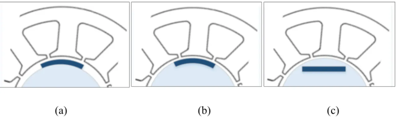
Fig. 2.2 Different types of magnet insertion: a) SPM, b) inset PM, c) Interior PM ... 9

Fig. 2.3. Distributed and concentrated windings [Cros, 2014] ... 10

Fig. 2.4. Segmented magnets in a SPM machine ... 10

Fig. 2.5. IGBT back to back converter ... 11

Fig. 2.6. Basic scheme of FOC [ST, 2007] ... 12

Fig. 2.7. Maximum torque control strategy ... 13

Fig. 2.8. Flux weakening control strategy ... 14

Fig. 3.1 a) A rotating disk in enclosure b) its flow regimes: regimes I & II represent laminar flows, regimes III and IV represent turbulent flows [Saari, 1998]. ... 22

Fig 3.2. Flowchart of the algorithm developed in [do prado, 2014].The input data (for Read File) is the flux density waveform B(t). ... 29

Fig. 3.4. Detected minor loops in the waveform of fig. 3.3. ... 31

Fig. 3.5. Flux density waveform from [do prado, 2014]. ... 31

Fig. 3.6. Detected minor loops in the waveform of fig. 3.5. ... 32

Fig. 3.7. Loci of the elliptical flux density harmonic ... 33

Fig. 3.8. Two simulated toroid cores (single lamination) ... 39

Fig. 3.10. a) Experimental set-up, b) laminated toroid ... 46

Fig. 3.11. Measured iron losses on the laminated toroid: a) 60 Hz 400Hz, b) 600 Hz 1 kHz, c) 2 kHz 5 kHz ... 48

Fig. 3.12. Measured iron losses on the laminated toroid under sinusoidal excitation (15

kHz, 30 kHz and 75 kHz) ... 49

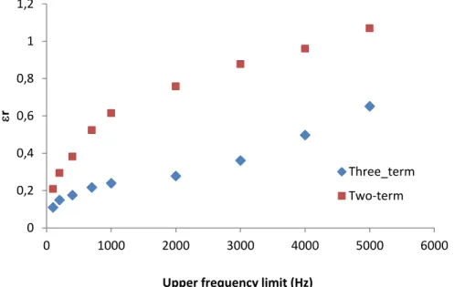
Fig. 3.13. Error function as a function of upper frequency range for two-term and three-term loss equations ... 50

Fig. 3.14 Measured losses (solid markers) compared to calculated losses with three-term Bertotti loss equation (solid trend line) and two term expression (dashed trend line) from 600 Hz to 1kHz (a) and 60 Hz to 400Hz (b) obtained with a single set of constant coefficients for the whole frequency range (60Hz-2kHz). ... 51

(12)

xii

Fig. 3.15. Measured losses (solid circle) compared to calculated losses (cross) with the three-term Bertotti loss equation (eq. (3.20), obtained with a single set of frequency dependent

coefficients for the whole frequency range (15 kHz-75kHz). ... 52

Fig. 3.16. Measured losses compared to calculated losses with the three-term Bertotti loss equation taking account of skin effect (eq. (3.22), obtained with a single set of frequency dependent coefficients for the whole frequency range (15 kHz-75kHz)... 52

Fig. 3.17. Calculated losses with the three-term Bertotti loss equation (solid trend line, eq. (3.22)) compared to calculated losses with two-term loss expression (dashed trend line, eq. (3.22) with Kex1=0, Kex2=0) obtained with a single set of frequency dependent coefficients for the whole frequency range (15 kHz-75kHz). The solid circles are measured losses. ... 53

Fig. 3.18. Magnetic field in one slot of the machine (generated by harmonic currents). .... 54

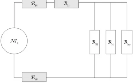
Fig. 3.19. The reluctance network for one slot of the machine. ... 55

Fig. 3.20. Permeability curve for various magnetizing frequencies ... 56

Fig. 3.21. Losses versus slot opening at no-load [Vu, 2013]. ... 57

Fig. 3.22. Eddy current path in non-segmented and segmented magnets ... 64

Fig. 4.1. General flow chart for design optimization methodology [Cros, 2014] ... 68

Fig.4.2. Computer-Aided- Design (CAD) environment with coupling of physical models [Cros, 2014]. ... 69

Fig.4.3. Flowchart of the design methodology [Cros, 2014] ... 71

Fig. 4.4. Determination of the concentrated winding of 8 poles 9 slots machine by applying the method in [Cros, 2002]. ... 75

Fig.4.5. Flowchart of the analytical design method of the motor structure [Cros, 2014] ... 76

Fig.4.6. Sectional view of a permanent magnet motor with external armature [Cros, 2014] ... 77

Fig. 5.1. Winding for the three-phase 9 slot 8 pole machine ... 85

Fig. 5.2 Position of the coils in stator slots of the 9 slot 8 pole machine ... 85

Fig. 5.3. The MMF space harmonic distribution of the winding in fig. 5.2. ... 86

Fig. 5.4. Stator lamination ... 89

Fig. 5.5. Completed stator winding ... 90

Fig. 5.6. Rotor I: Non-segmented Magnet and steel yoke (430 type) ... 91

Fig. 5.7. Rotor II : Segmented magnets and laminated rotor core ... 91

Fig. 5.8 The Kevlar sleeve for the first rotor (Rotor I) ... 91

Fig. 5.9. Assembly of the stator in the aluminium housing. ... 92

Fig. 5.10. Position of thermocouples [Kirouac, 2015] ... 93

Fig. 5.11. Motor-generator and encoder assembly ... 93

(13)

xiii

Fig. 5.13. Schema for the converter power circuit [Ivankovic, 2007] ... 95

Fig. 5.14. Interface card and eZdsp™ F2812 development kit ... 96

Fig. 5.15. The block diagram of the field oriented control of the machine [Ti, 2003] ... 96

Fig. 5.16. The schema for experimental set-up ... 97

Fig. 5.17. Experimental set-up for the two PMSMs (in the same housing) ... 98

Fig. 5.18. No-load losses of the test bench machines (motor-generator) as a function of air temperature in the space between two rotors... 99

Fig. 5.19. Total losses measured in the test bench machines (V DC-link=400 V, maximum torque, at Tref=39.5 °C) ... 100

Fig. 5.20. The stator current for filtered (a) and unfiltered (b) PWM supply measured at 5000 RPM (V DC-Link= 400 V) ... 101

Fig. 5.21. The harmonic content of the filtered and unfiltered stator currents at V DC-Link= 400 V, f0 =333.33 Hz , fc=15 kHz (f0 is the fundamental frequency). ... 101

Fig. 5.22. Total input losses for two machines with filtered and unfiltered supplies, V DC-link=400 V at Tref=39.5 °C. ... 102

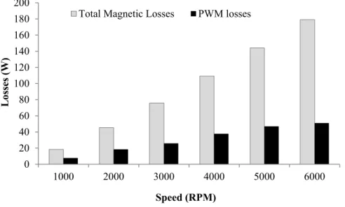
Fig. 5.23. Total magnetic losses in the motor compared to PWM magnetic losses for various speeds, VDC-link=400 V at Tref=39.5 °C. ... 103

Fig. 5.24. Total losses in the two machines under variable DC bus voltage, 5000 RPM, Tref=39.5 °C ... 104

Fig. 5.25. PWM losses in the motor (after separation) for a variable DC bus voltage, 5000 RPM, Tref=39.5 °C ... 105

Fig. 5.26. Separation of PWM losses in stator, magnets, and rotor core (Rotor I) under variable DC-link voltages at 15 kHz carrier frequency. ... 105

Fig. 5.27. The harmonic content of the stator current for 250 V and 400 V (DC-Link voltages) at 15 kHz carrier frequency (f0 =333.33 Hz). ... 106

Fig. 5.28. PWM losses (after separation) for a variable carrier frequency at 5000 RPM, V DC-link=400 V, Tref=39.5 °C ... 107

Fig. 5.29. Separation of PWM losses in stator, magnets, and rotor core for a variable carrier frequency at 5000 RPM, VDC-link=400 V, Tref=39.5 °C ... 107

Fig. 5.30. The harmonic content of the stator current for a variable carrier frequency at 5000 RPM, VDC-link=400 V, Tref=39.5 °C ... 108

Fig. 5.31. Losses in the two machines (Exp.) and total losses in the converter and machines (Pdc) measured from 1000 to 5000 RPM (Iq,g12.5 A, maximum torque, VDC-link=400 V). ... 109

Fig. 5.32. Losses in the two machines (Exp) and total input losses in converter and machines (Pdc) as a function of d-axis current (5000 RPM, VDC-link=400 V, Iq,g=0.5 pu , 1 pu = 25 Arms). ... 110

(14)

xiv

Fig. 5.33. Losses in the two machines (Exp.) and total losses in the convertor and machines (Pdc) measured from 5500 to 7000 RPM (Is,g12.5 A, VDC-link=400 V) shown along with the

results from fig. 5.31 for the maximum torque region. ... 111 (a) ... 116 Fig. 6.2. a) Model of the 9 slot 8 pole machine, b) Finite-element mesh and c) the grid used for the tooth and back iron. ... 116 Fig. 6.3. Grid used for the rotor II core (with segmented magnets) ... 117 Fig. 6.4. Current source for the 2D-FE model ... 118 Fig. 6.5. a) Experimental no-load stator current and b) its harmonic analysis (5000 RPM, VDC-link=400V, maximum torque, fc=15 kHz, f0=333.33 Hz). ... 119

Fig. 6.6. The reconstructed stator current (5000 RPM, VDC-link=400V, maximum torque,

fc=15 kHz, f0=333.33 Hz). ... 120 Fig. 6.7. Electrical circuit for the permanent magnets and solid rotor core for Rotor I (with non-segmented magnets and solid rotor core) ... 122 Fig. 6.8. Electrical circuit for the permanent magnets and solid rotor shaft for Rotor II (with segmented magnets) ... 122 Fig. 6.9. Bearing losses as a function of machine speed for two bearings ... 124 Fig. 6.11. Relation between Couette Reynolds number and friction coefficient in turbulent and laminar regimes for the analysed machine (1000-8000 RPM) ... 126 Fig. 6.12. Comparison of friction losses in the air gap calculated with equations (3.5-3.8) versus results obtained with equations (3.9-3.10) ... 126 Fig. 6.13. Friction Losses in the end surfaces of the rotor when considered as rotating disks in free space (blue); when considered as rotating disks in enclosure (red). ... 127 Fig. 6.14 Radial and peripheral components of flux density for the point shown in the tooth tip at 5000 RPM , no-load condition. ... 128 Fig. 6.15. Detection of minor loops and their amplitudes according to algorithm presented in chapter 3 for the peripheral component of the flux density waveform in fig. 6.14. (‘delta’ is the minor loop peak to peak amplitude and ‘pks’ represents the local peaks). ... 129 Fig. 6.16. Distribution of total hysteresis losses (in W/m3) due to major and minor loops at 5000 RPM (Iq,g=12.5 A, maximum torque ... 130

Fig. 6.17. Distribution of losses (in W/m3_{) due to minor hysteresis loops (right) at 5000 RPM}

along with the radial and peripheral components of the flux density in various parts of the machine under load (Iq,g=12.5 A, maximum torque). ... 131

Fig. 6.18. Distribution of losses (in W/m3_{) due to major hysteresis loop at 5000 RPM}

(Iq,g=12.5 A, maximum torque). ... 131 Fig. 6.19. The hysteresis losses calculated according to their origins in the frequency and time domains at 5000 RPM (Iq,g=12.5 A, maximum torque). ... 132

(15)

xv

Fig. 6.20 Harmonic magnetic losses in the motor stator at 5000 RPMat no- load (Is,m=1.25

A, maximum torque, VDC-link=400 V) ... 134

Fig. 6.21 Harmonic magnetic losses in the motor stator at 5000 RPM under load (Iq,g=12.5

A, maximum torque, VDC-link=400 V) ... 134 Fig 6.22. Estimated losses in the motor and generator with 2-term and 3-term loss expressions in the time and frequency domain, compared to experimental test at 5000 RPM under load (Iq,g=12.5 A, maximum torque, VDC-link=400 V). ... 136 Fig.6.23. Losses in the two machines with 2-term and 3-term loss expressions in the frequency domain separated according to their origins into magnetic stator losses (Ph1, Ph3-7,

Ppwm) and other losses (mechanical, rotor losses) at 5000 RPM under load (Iq,g=12.5 A,

maximum torque, VDC-link=400 V). ... 137

Fig. 6.24. Estimated losses in the motor and generator with 2-term and 3-term loss expressions in the time and frequency domain, compared to experimental test at 5000 RPM at no- load (Is,m=1.25 A, maximum torque, VDC-link=400 V). ... 137 Fig. 6.25. No-load losses in the two machines with 2-term and 3-term loss expressions in the frequency domain magnetic stator losses (Ph1, Ph3-7, Ppwm) and other losses (mechanical,

rotor losses) at 5000 RPM (Is,m=1.25 A, maximum torque, VDC-link=400 V). ... 138 Fig. 6.26. The main high frequency current harmonics generated by the PWM supply obtained with harmonic analysis of the measured input current (1000-7000 RPM, maximum torque, VDC-link=400 V). ... 139 Fig. 6.27. The scatter type (a) and column type (b) charts for total calculated no-load losses compared to experimental test for the test bench machines (1000-7000 RPM, maximum torque, VDC-link=400 V). The distribution of magnetic losses in the stator of the motor

according to their origins in the frequency domain (Ph1, Ph3-7, Ppwm) are also shown for each

speed (b). ... 140 Fig. 6.28. PWM losses obtained with experimental test (after the separation of rotor losses) compared with calculated PWM losses in the stator of the motor at 1000- 5000 RPM (at no-load, maximum torque, VDC-link=400 V). ... 141

Fig. 6.29. The main PWM supply harmonics obtained with harmonic analysis of the measured input current (Iq,g12.5 A, maximum torque, VDC-link=400 V). ... 142

Fig. 6.30. The scatter type (a) and column type (b) charts for total calculated losses compared to experimental test for the test bench machines under constant torque (Iq,g12.5 A,

maximum torque, VDC-link=400 V). The distribution of magnetic losses in the stator of the

motor according to their origins in the frequency domain (Ph1, Ph3-7, Ppwm) are also shown for

each speed. ... 143 Fig. 6.31 Distribution of magnetic and copper losses in the stator and rotor of the motor calculated for each speed (Iq,g12.5 A, maximum torque, VDC-link=400 V). ... 144 Fig. 6.32. The total calculated losses compared to experimental test for the test bench machines for different values of d-axis current (Iq,g=0.5 pu , 1 pu =25 Arms).The distribution

(16)

xvi

domain (Ph1, Ph3-7, Ppwm) are also shown for each current (5000 RPM,

VDC-link=400 V) ... 145

Fig. 6.33. Distribution of magnetic and copper losses in the stator and rotor of the motor at 5000 RPM as a function of d-axis current (Iq,g=0.5 pu , 1 pu = 25 Arms). ... 145 Fig. 6.34. The total calculated losses (cal.) compared to experimental results (Exp) for the two machines in the maximum torque and flux weakening regions (Is,g12.5 A, VDC-link=400

V, constant power). Measurement uncertainty (Uncert.) is calculated using the specifications of the power analyser. ... 146 Fig. 6.35. The distribution of magnetic losses in the stator of the motor according to their origins in the frequency domain (Ph1, Ph3-7, Ppwm) calculated for each speed (Is,g12.5 A, V DC-link=400 V, constant power) ... 147

Fig. 6.36. Distribution of magnetic and copper losses in the stator and rotor of the motor calculated for each speed (Is,g12.5 A, VDC-link=400 V, constant power) ... 148

Fig. 6.37. The main PWM supply harmonics obtained with harmonic analysis of the measured input current for each speed (Is,g12.5 A, VDC-link=400 V, constant power). ... 148 Fig. 6.38. The total calculated no-load losses in the test bench machines compared with experimental results for a variable DC-link voltage. The experimental PWM-losses (Exp-PWM) of the motor after separation and calculated PWM losses (Cal-(Exp-PWM) are also shown (5000 RPM , fc=15 kHz, maximum torque). ... 149

Fig. 6.39. The distribution of magnetic losses in the stator of the motor according to their origins in the frequency domain (Ph1, Ph3-7, Ppwm) along with rotor losses (Protor) for a variable

DC-link voltage (5000 RPM , fc=15 kHz, maximum torque). ... 150 Fig. 6.40. Magnetic losses due to PWM harmonics in the motor stator at 5000 RPM at no-load for a variable DC-link voltage (5000 RPM , fc=15 kHz , Is,m1.25 A, maximum torque)

... 151 Fig. 6.41. The total calculated no-load losses in the test bench machines compared with experimental results for a variable carrier frequency. The experimental PWM-losses (Exp-PWM) of the motor after separation and calculated PWM losses (Cal-(Exp-PWM) are also shown (5000 RPM , VDC-link=400 V, maximum torque). ... 152 Fig. 6.42. Magnetic losses due to PWM harmonics in the motor stator at 5000 RPM at no- load for a variable carrier frequency (5000 RPM, Is,m1.25 A, maximum torque, VDC-link=400

V) ... 153 Fig.6.43. Stator PWM iron losses at 250V (b) and 400V (a) DC-Link voltages and fixed carrier frequency (fc=15 kHz) obtained with analytical method compared to simulation

results by 2D-FE (method (4)). ... 154 Fig. 6.44. Total stator PWM iron losses under variable DC-Link voltages and fixed carrier frequency (15 kHz) obtained with analytical method compared to simulation results by 2D-FE (method (4)). ... 155 Fig. 6.45 Stator PWM losses: analytical model, 2D-FE for a variable carrier frequency at 400 V DC-Link voltage. ... 156

(17)

xvii

Fig. 6.46. Eddy current losses predicted with the new approach (2D FEA Eq. (3.48)), Eq. (3.44), and the classical eddy current loss expression (Eq. (3.32)) at 30 kHz... 158 Fig. 6.47. Eddy current losses calculated with the new approach (eq. (3.48) ) compared with losses estimated with eddy current loss term in equation (3.22). ... 158 Fig. 6.48. Magnetic field in the machine stator ... 159 Fig. 6.49. Loci of the flux density in various zones of the stator ... 160 Fig. 6.50 Eddy current losses at no-load obtained by eq. (3.48) for tooth and yoke regions compared to losses calculated by eddy current loss term in eq. (3.32) at 5000 RPM, (no-load, maximum torque). ... 161 Fig. 6.51 Eddy current losses under load obtained with eq. (3.48) compared to losses calculated by eddy current loss term in eq. (3.32) at 5000 RPM, (Is,m=13.67 A, maximum

torque). ... 161 Fig 6.52. Orthogonal components of flux density at rotor surface (left) and their harmonic content (right) for generator (no-load, 5000 RPM). ... 163 Fig 6.53. Orthogonal components of flux density at rotor surface (up) and their harmonic content for low order harmonics (middle) and the high order harmonics for the radial component of the flux density (bottom) for motor under load at 5000 RPM (Iq,g=12.5 A,

maximum torque, VDC-link=400 V). ... 165

Fig. 6.54. Harmonic magnetic losses in the rotor laminations of the motor at 5000 RPM under load (Iq,g=12.5 A, maximum torque, VDC-link=400 V) ... 165 Fig. 6.55. Harmonic magnetic losses around 30 kHz (2fc) in the rotor laminations of the

motor calculated with and without skin effect compensation at 5000 RPM under load (Iq,g=12.5 A, maximum torque, VDC-link=400 V). ... 166 Fig 6.56. The total calculated losses (by 2D FE) under load in the test bench machines (with segmented magnets) compared with experimental test (a). The calculated losses in the magnets and solid rotor core of the motor under load (rotor I) are compared with the calculated losses in the laminated rotor and segmented magnets (rotor II) (b). ... 167 Fig 6.57. The total calculated losses (by 2D FE) at no-load in the two machines (with segmented magnets) compared with experimental test (a). The calculated losses in the magnets and solid rotor core of the motor at no-load (rotor I) are compared with the calculated losses in the laminated rotor and segmented magnets (rotor II) (b). ... 167 Fig. 6.58. Eddy current losses generated in the magnets of the first rotor (a) and in the segmented magnets of the second rotor (b) as a result of the interaction between time and space harmonics of the stator winding (motor at 5000 RPM, under load, maximum torque, Iq,g=12.5 A, VDC-link=400 V). ... 169

Fig. 6.59. Eddy current losses in the magnets of rotor I (non segmented) calculated with 2D-FE compared to those calculated with analytical method for various harmonic currents (only fundamental, only harmonic 89, all harmonic currents), (motor at 5000 RPM, under load, maximum torque, Iq,g=12.5 A, VDC-link=400 V). ... 170

Fig. 6.60. Eddy current losses in the magnets of rotor II (segmented) calculated with 2D-FE compared to those calculated with analytical method for various harmonic currents (only

(18)

xviii

fundamental, only harmonic 89, all harmonic currents), (motor at 5000 RPM, under load, maximum torque, Iq,g=12.5 A, VDC-link=400 V). ... 170

(19)

xix

List of Symbols and Abbreviations

Alphabetic symbols

A Specific armature loading

B Flux density

B, Bteta Peripheral component of flux density

Ba Air gap flux density

Bdc DC induction level of the flux reversal

BLV,min Deepest flux density valley at the left side of a local peak

Bm Peak flux density

Bm Amplitudes of hysteresis cycles in the waveforms of the peripheral

component of the flux density

Bmag Iron flux density

Bmin,n , Bmax,n Major and minor axes of the flux density locus for harmonic n

Bmr Amplitudes of hysteresis cycles in the waveforms of the radial component

of the flux density

Bn Flux density amplitude for harmonic n

Bp Local peak flux density

Br Radial component of flux density

Bre Residual induction

BRV,min Deepest flux density valley at the right side of a local peak

Bsat Iron flux density saturation threshold

(20)

xx

Cf Friction coefficient

Cfb Constant coefficient of friction for bearing

d Lamination thickness

D Stator internal diameter

db Bearing bore diameter

dc Density of the coolant

De Slot diameter

Dext External diameter of the machine

Dint Inner diameter of the machine

Dr Rotor diameter

Dsh Shaft diameter

eca Armature yoke thickness

ecr Permanent magnet yoke thickness

etb Tooth tip thickness

F Equivalent dynamic bearing load

f Frequency

f0 Fundamental frequency

Fa Axial component of the bearing load

fc Carrier frequency

Fr Radial component of the bearing load

fr Frequency in the rotor reference frame

fsl Frequency of the rotor eddy currents due to slot harmonics

g Air gap thickness

I Current

Ih Amplitude of the harmonic current

Iph, Is Phase current

Iq, g Generator q-axis current

iq, id Currents in the q and d axes

Is,g Stator current for generator

Is,m Stator current for motor

isD, isQ Orthogonal components of current in the stator reference frame

isq, isd Orthogonal components of current in the rotating reference frame

isqref, isdref Reference values for orthogonal components of current in the rotating

reference frame

Iu Amplitude of harmonic u current

J Current density

(21)

xxi

Ked, Ked1, Ked2 Eddy current loss coefficients

Kex, Kex1, Kex2 Excess loss coefficients

Kfb Bearing friction coefficient

Kh Hysteresis loss coefficient

Kr Copper filling factor

kro Roughness coefficient

Ksov Slot opening factor

Kw Winding coefficient

Kwv Winding coefficient for space harmonic 

L Rotor length

l Lamination or magnet length

la Magnet thickness

lavg Average magnetic path

Lind Inductance

Lmax Maximum axial length of the motor

Lturn One turn length per coil for an external armature

mph Number of phases

mr Mass of the rotor

N Speed NE

Np

Number of finite elements Number of time steps per period

Nph Number of series turns per phase

Ns Number of series turns per coil

Nseg Number of magnet segments

p Number of pole pairs

Pb Bearing losses

Pcal Calculated losses

Pcu Copper losses

Ph1, Ph3-7, Ppwm Magnetic loss components in the frequency domain

Pmeas Measured losses

ps Number of stator poles

Pρw1 Gas friction losses in the air gap

Pρw2 Gas friction losses in the end disks of the rotor

Qs Number of slots

R Stator internal radius

Rag Reluctance for air gap

(22)

xxii

Rea Reynolds number for axial flux in the air gap

Reg Couette Reynolds number

Rer Tip Reynolds number

rhn Ratio of hysteresis losses under circular rotating field to hysteresis losses

under alternative field

Rlk Reluctance for flux leakage

Rm Magnet outer radius

Rph Phase resistance

Rr Magnet inner radius

Rso Reluctance for slot opening

Rth Reluctance for tooth

Rtt Reluctance for tooth tip

s Axial clearance between the rotor ends and the enclosure

Scu Total copper section

Spp Number of slots per pole and per phase

T Electric period

Tb Bearing operating temperature

Te Torque

Tem Electromagnetic Torque

Temp Temperature

Tg Air gap temperature

Tref Reference temperature

Tw Working temperature

u Order of time harmonic

v Order of space harmonic

VDC-link DC link voltage

Vph Phase voltage

w Lamination or magnet width

Wan Hysteresis losses under alternating field

Wed Eddy current loss volumic density

Wex Excess loss volumic density

Wh Hysteresis loss volumic density

Wied Total eddy current losses in the iron volume

Wiex Total excess losses in the iron volume

Wih Total hysteresis losses in the iron volume

Wrn Hysteresis losses under circular rotating field

(23)

xxiii

Greek Symbols

 Skin depth

 Angle between the Br vector and the positive x-axis in the xy plane

t Tooth angular width

 Magnet pole arc

 Minimal efficiency

 Dynamic viscosity of the coolant

a Armature reaction flux

d d-axis flux linkage

f A coefficient depending on iron characteristics

m Electrical resistivity of the magnets

m Mean axial fluid velocity

n Axis ratio

n Flux density phase for harmonic n

PM Permanent magnet flux

q q-axis flux linkage

r Rotor angular speed

v No-load flux per phase

αcu The temperature coefficient of resistivity

ΔBi

t

Peak to peak amplitude of the minor hysteresis cycle i Time interval

ΔVi Volume of element i

μ Absolute permeability

 Lamination resistivity

cu Copper resistivity

x, z Lamination resistivity in the x and z axes

Ω Angular frequency

Abbreviations

(24)

xxiv

3D Three Dimensional

ADC Analog to Digital Converter

CAD Computer Aided Design

CAO Computer Aided Optimization

DSP Digital Signal Processor

FE Finite Element

FEA Finite Element Analysis

FOC Field Oriented Control

GCD Greatest Common Divisor

IPM Interior Permanent Magnet

LCM Least Common Multiple

MMF PF

Magneto-Motive Force Power Factor

PM Permanent Magnet

PMSM Permanent Magnet Synchronous Machine

PWM Pulse Width Modulation

RPM Rotation Per Minute

SMPM Surface Mounted Permanent Magnet

SPWM Sinusoidal Pulse Width Modulation

VA Volt-Ampere

(25)

xxv

Acknowledgements

It is not easy to find the right words to thank my supervisor Jérôme Cros for his exceptional qualities as a wonderful person and also as an excellent pedagogue with a vast knowledge in electrical machines. I particularly appreciate his availability, willingness to assist with all issues, his knowledge and his understanding. Without his continuous support, his guidance, and his patience, this work was not possible. It has been an great privilege to have known him and to have worked as his student.

I would also like to express my gratitude to Maxime Dubois who initially gave me the chance to begin my PhD studies and for his support. I would also like to thank Philippe Viarouge, for his contagious passion and for being a source of inspiration for all students in electrical machines. It has also been a great pleasure to attend the courses of Mr. Hoang Le-Huy as an excellent pedagogue and read his valuable textbooks. I also wish to thank Mr. Stephane Clenet and other jury members for taking the time to read this work and for their valuable suggestions and encouragement.

Also thanks to all my LEEPCI colleagues for such a nice experience, and to Marco Béland for his role in building the prototype machine. My deepest gratitude, however, goes to my exceptional wife, Farideh, for her encouragement and support through such a long project, and for her great understanding.

(26)

1

Chapter 1: Introduction

The huge energy consumption at an unprecedented pace, and its environmental consequences, are a global concern in the modern days. As a result, all measures and technical innovations which could contribute to more efficient use of energy are greatly appreciated. Electric machines are so widely used that small improvements in the efficiency of the machine will bring about important economies in electrical energy.

Already in 2004, there were more than 700 million motors in service worldwide and approximately 50 million new motors manufactured every year [Emadi, 2004]. According to [ABB, 2015], 42% of all electricity used powers industry. Two third of this electricity is used for electrical motors. This means that 28% of the global electrical energy consumption is used for the electrical machines (21.9 trillion kWh en 2015). For their part, the electrical generators produce the majority of this electricity (around 86%). A simple calculation (based on the data in 2012) shows that an improvement of 1% of the efficiency of the electrical machine will save us the equivalent of the 10% of all the production of nuclear plants. In this calculation, the electrical motors in residential sector (the compressors, fans and pumps) are not considered.

According to [ABB, 2015], improved design can increase the efficiency of individual motors by up to 30%. For an improved design, modelling the losses plays a leading role. Implementation of accurate models (particularly in the case of magnetic losses), will be a

(27)

2

very precious tool for the machine designers which often use simplified models for loss estimation in the design process.

We may optimize the machine if only we have accurate loss models for all operating conditions. This is particularly important for the magnetic losses which will be the main focus of this work. The PWM inverters are widely used to drive permanent magnet synchronous machines (PMSMs). While these inverters have many advantages, they may also generate significant eddy current losses in the magnets and iron losses in the stator and rotor laminations. The accurate estimation of iron losses due to harmonics present in the PWM supplies by FE models is not a simple task. Normally, the existing loss models, do not take into account the high frequency effect associated with a PWM supply. This may result in highly exaggerated estimations of iron losses in the machine if the skin effect is present. In this work, we will explore this aspect by experimental measurements and by employing finite-element modeling software. The objective of this approach is to develop simple models that can be used in the loss analysis and CAO process for electrical machines.

1.1 Thesis outline

Chapter 2 is an overview of the permanent magnet machine. In this chapter a very brief description of various structures of the permanent magnet machine, converter and its control strategies is presented. Only details which are necessary for understanding the different aspects of the experimental set-up and its operation conditions are presented. For example only maximum torque and flux-weakening control strategies are examined since they will be later applied for the test bench machines.

In chapter 3, the models for the prediction of various types of losses in a permanent magnet machine including the mechanical losses, copper losses and magnetic losses will be examined. The magnetic losses, as the focus of this work, will be examined in more detail. The magnetic losses have by far the largest share of losses in the machine at no-load condition. In the loaded condition, on the other hand, both magnetic and copper losses may generate significant losses in the machine. However, compared to magnetic losses, the estimation of copper losses is a simpler task if the copper temperature is known. The

(28)

3

mechanical losses normally comprise a small share of the losses, nevertheless, their modeling will be examined carefully. In the case of fractional machines with concentrated windings, the stator MMF might be rich in harmonics and the rotor losses could also be significant. Although, the losses might still be smaller than stator losses, however, losses in the rotor are more difficult to evacuate and the heat buildup in the rotor may cause irreversible demagnetization of the magnets. Exceeding the temperature limit of the magnet retaining sleeves can also cause important damage to the machine. Therefore, in this chapter, the estimation of rotor losses is also treated with great care.

The magnetic losses are usually separated into hysteresis, eddy current and excess losses (three-term approach), however, in many recent research works, the excess losses are combined with the classical eddy current losses to form a single global eddy current loss term (two-term approach). As will be shown later (in the case of a machine and a laminated toroid), the choice of the separation method will affect the accuracy of the loss estimation. Therefore, this comparison will help the designer to select the appropriate method for a better accuracy. Various models for hysteresis, eddy current and excess losses (in the time and frequency domains) will be discussed separately. As for hysteresis losses, an algorithm for the identification of the minor hysteresis cycles will be presented.

The Bertotti expression for iron losses may be considered as the most widespread model for the estimation of magnetic losses in the laminations and is integrated in many commercial software packages for loss estimation in the post-processing stage. However, this expression is not valid if the skin effect is present in the laminations (which may be the case at high switching frequencies in PWM supplies). Therefore, in chapter 3, a new loss expression for taking account of the skin effect in a laminated magnetic material will be introduced. Also, extensive measurements in a wide range of frequencies and magnetic flux densities on a toroid made from the same material as the stator of the prototype machine (in chapter 5) are used to identify the loss coefficients for the loss expressions presented in this chapter. These loss coefficients are necessary later (in chapter 6) for accurate estimation of losses in the lamination material by the 2D-FE simulation models. Also, as a more practical alternative in the design stage, an analytical model is presented which may serve as a valuable tool for the estimation of the PWM losses in the stator of a permanent magnet machine. Besides, a new

(29)

4

method for the direct estimation of eddy current losses in the lamination material by 2D-FE analysis is also presented in which the laminations are modelled as conductive material. In chapter 4, the design methodology for a surface mounted permanent magnet (SMPM) machine is presented. The procedure for the design of armature winding, the optimization method and the associated analytical design models are also presented and some design considerations like the choice of the lamination material, the effect of manufacturing process on losses and heat removal techniques will be briefly examined.

The procedure for the design of a SMPM machine in chapter 4, is used to design the prototype machine in chapter 5. The machine structure will be selected as the first step. The machine required specifications will then be used as constraints in the optimization process and the final results of the CAO will be used to realize two identical machines for an innovator experimental test bench. A second rotor with segmented magnets and laminated rotor yoke will also be constructed to study the effect of the segmentation and the rotor yoke material on the rotor losses. A detailed description of the machine construction and assembly is also presented. The test bench will then serve as a platform for measuring machine losses in a variety of operating conditions and speeds.

Chapter 6 will be mainly dedicated to the analysis of losses and validation of the loss models presented in chapter 3 using the experimental results presented in chapter 5. The details concerning the 2D-FE simulation model, the procedure for the simulation of the stator current, estimation of losses in the post-processing stage, and modeling of magnet and rotor core are also presented. The mechanical losses are calculated in the test bench machines. The algorithm presented in chapter 3 for the detection of minor loops is applied to the stator of the machine to identify the minor loops and calculate their respective losses. The results of total losses for both minor and major loops are also compared with those obtained with the harmonic analysis of the flux density waveforms.

In order to find the most appropriate method, various models for magnetic losses with or without skin effect consideration, in the time or frequency domains, and with 2-term or three-term separation methods are compared. The method with the best estimations is then validated in a wide range of operating conditions as follows:

(30)

5  No-load, variable speed

 No-load, fixed speed, variable modulation frequency  No-load, fixed speed, variable DC-link voltage  Constant torque, variable speed

 Constant speed and torque, variable current phase angle (for identification of optimal efficiency phase angle for stator current)

 Variable speed -constant power (flux weakening) driving zone

Such a rigorous validation will ensure that the models are reliable and their performance is not the result of coincidence.

Besides, in this chapter, the stator PWM losses estimated by the analytical method (introduced in chapter 3) are compared to those calculated with 2D-FE for a variable DC-link voltage and a variable modulation frequency. The new approach for direct eddy current loss estimation is also validated in the case of laminated toroid and will be then applied to the prototype machine.

Finally, the losses in the rotor yoke and magnets of the two rotor (with or without segmentation) will also be compared and the effect of segmentation and the choice of rotor yoke (solid iron versus laminated) on the rotor losses are investigated. The results will be then compared with those of the analytical model presented in chapter 3.

(31)

6

Chapter 2: An Overview of the

Permanent Magnet Machine

2.1 Introduction

Permanent magnet (PM) synchronous machines are becoming more and more popular because of the many advantages they offer. They have become an attractive choice for replacing other machine types (e.g., induction machines) due to their advantages and also due to the reduction in the price of the new performing permanent magnets. Some of the main advantages of the PM synchronous machine are summarized below:

 It offers high torque densities and requires no field excitation (unlike wound rotor synchronous machine).

 Rotor losses are lower compared to other machine types (asynchronous, wound rotor synchronous)

 High efficiencies can be obtained with proper design.

There are also a number of disadvantages associated with the use of PM synchronous machines:

 The magnets will generate losses in the stator of the machine at no-load conditions.  Permanent magnets can be demagnetized if over-heated.

(32)

7

 In an internal rotor structure with surface mounted magnets, retaining sleeves are required.

 Some magnet types are conductive, therefore, in some machine structures, important eddy-current losses may be generated in the rotor (e.g. fractional slot concentrated winding machine). This increases the risk of demagnetization.

Solutions to overcome these disadvantages already exist. For example, magnet losses can be reduced by magnet segmentation. The rotor losses can also be reduced by the appropriate choice of the winding configuration. The magnetic losses can also be reduced by flux-weakening (though the copper losses will increase).

The internal rotor machines with interior permanent magnets and external rotor structures do not need the retaining sleeves. Besides, retaining the magnets in the conventional surface mounted magnets is not a major problem due to the availability of the new high strength materials for the retaining sleeves (e.g. carbon fibre composite) The use of composite material for the sleeves will reduce the thermal dissipation of the rotor since they do not generate eddy current losses.

2.2 Structures

PM machines are classified according to the direction of air-gap flux into axial or radial flux machines. In this work, only the various structures for the radial flux machines will be considered.

2.2.1 External rotor versus internal rotor

The internal rotor is the most common configuration used for a PM synchronous machine. An important advantage of this configuration is the fact that removing the heat generated in the stator is a straight forward task (since the stator yoke is in contact with the air).

The main advantage of the external rotor is a higher torque density compared to an internal rotor machine. In additions, it does not need a retaining sleeve. The disadvantage of such a

(33)

8

configuration is that the mechanical assembly will be more complicated. Also, the connection of the stator winding terminals will be no easy task. Besides, the heat dissipation will be a major challenge since the losses are mainly generated in the stator.

Fig. 2.1. Internal and external rotors

2.2.2 Interior and surface mounted magnets

PM synchronous machines are also classified according to the position of the magnets in the rotor into three main types: surface permanent magnet (SPM) machines, inset PM machines, and interior PM (IPM) machines as shown in fig. 2.2.

The SPM (or SMPM) machine is the most widely used machine among these three types. The insertion of magnets for this machine is not a difficult task in the manufacturing process, however, as mentioned before, retaining the magnets on the rotor surface by means of sleeves is necessary to protect them from centrifugal forces which can be very important at high speeds and high rotor diameters.

The IPM machine, on the other hand, is gaining a lot of attention due to two main reasons. First, it does not need a retaining sleeve, and second, it is well adapted for constant power operation in a wide speed range by flux-weakening strategy [Yamazaki, I, 2010], [Jahns, 1987]. However, the use of IPM rotors may result in increased magnetic losses in the stator particularly under the flux-wakening operation [Yamazaki, I, 2010].

(34)

9

(a) (b) (c)

Fig. 2.2 Different types of magnet insertion: a) SPM, b) inset PM, c) Interior PM

2.2.3 Winding

The two main winding types used in the PM machine are the distributed and concentrated windings (fig. 2.3). Among the two, the distributed windings are the more widely used winding type in conventional machines. The use of concentrated windings, on the other hand, has been limited to applications of sub-fractional power [Cros, 2002].

In [Cros,1999], the authors showed that by using a concentrated winding and a proper selection of slot and pole number combination, a high winding coefficient and subsequently high torque can be obtained. Since then, the concentrated winding machines have received a lot of attention in the literature and have become increasingly popular because of their numerous advantages. Their winding structure is simple and well adapted for automated manufacturing (therefore lower manufacturing cost) or stator segmentation. They have short end windings which means they use less copper in the end windings [Cros, 2002]. They also reduce the risk of short-circuit between windings of two phases [Wang, 2014]. Besides, some structures with concentrated windings have lower cogging torque and, therefore, do not need slot skewing [Cros, 2002].

Their most important drawback is the fact that the armature reaction field may contain significant space harmonics which can generate important losses in the rotor, at high speed. Nevertheless, this can be remedied by segmentation of the magnets (fig. 2.4) and proper selection of the rotor core material as will be shown later in the design of our prototype, in chapter 5.

(35)

10

Fig. 2.3. Distributed and concentrated windings [Cros, 2014]

Fig. 2.4. Segmented magnets in a SPM machine

2.3 Converter

Different AC-AC converter topologies could be used to drive a PM synchronous including the direct and indirect converter topologies. Matrix converter [Toliyat, 2006], is an example of direct converter topology, in which, the inputs and outputs are connected through bi-directional switches. The main advantage of such a topology is the fact that it does not need a DC-link (therefore no energy storing components are required). However, this topology necessitates a high number of power semiconductors (in its basic version: 6 IGBTs for each phase) and is less commonly used in industry.

In the AC-AC indirect converter topologies, the AC mains or the output of a generator is first converted to DC by means of a rectifier and then converted again to AC by means of an inverter. The most common inverter topology used in the industry is a two-level PWM-VSI

(36)

11

(Pulse Width Modulated Voltage Source Inverter) which uses only 2 switches per phase (or per one leg of the inverter). By use of controlled switches like IGBTs or MOSFETs the power transfer can be bi-directional which means that each bridge may function as inverter or rectifier. IGBTs are more widely used, however, they have high conduction losses. As an alternative, MOSFETs in parallel can be considered, however, the complexity of their implementation, their lower reliability, and their rather low breakdown voltages (compared to IGBTs) are important drawbacks. Figure 2.5 shows an AC-AC converter with bidirectional power flow (with IGBT switches) often called a back to back converter.

Fig. 2.5. IGBT back to back converter

Different PWM modulation techniques can be used to drive the bridge. The two most widely used PWM modulation schemes are SPWM (Sinusoidal PWM) and SVPWM (Space Vector PWM). It should be noted that the choice of topology and modulation scheme will not only affect the converter losses, it may also have a non-negligible effect on the machine losses. The effect of PWM supply parameters on machine losses will be discussed in chapter 5 and chapter 6.

2.4 Converter control

The availability of powerful microcontrollers will allow us to implement complex control schemes. One of the most widely used control schemes for PM machines is the flux oriented control (FOC) [Ti, 2013 ]. In this section, this type of machine control along with two main control strategies will be presented.

(37)

12

2.4.1 Field Oriented Control (FOC)

The FOC allows the separate control of q axis current which produces the torque and d axis current which controls the demagnetising flux. As could be seen in the basic scheme of the FOC in fig. 2.6, the Clarke transformation is applied to measured phase currents to find the orthogonal components of current in the stator reference frame (isD, isQ). Park transformation

is then used to find the orthogonal components of current in the rotating reference frame (isq,

isd). The rotor position data (angle e) is required at this point, for the Park transformation.

The results of transformation are then compared with the reference values (isqref, isdref) for

torque and flux control. The outputs of the two regulators (usqref, usdref) are then applied to

inverse Park transformation to find the orthogonal components of the stator voltage in the stationary reference frame. These voltages serve as reference for the PWM generator which generates the PWM signals for the inverter drivers.

(38)

13

2.4.2 Machine control strategies

The decoupling of torque and magnetization, as shown in the previous section, allows us to easily implement the two main control strategies for PM machine: maximum torque and flux weakening. Though, various other control strategies exist [Toliyat, 2005], only these two main types will be presented. It should be mentioned that the choice of control strategy will affect both the machine and converter losses and the VA rating of the converter.

2.4.2.1 Optimum torque per ampere control

In a PM synchronous machine with non-salient poles, we have:

T p Φ i Φ i (2.1)

where p is the machine pole pair number and d, q , iq and id are the flux linkage and currents

in the d and q axes. As could be seen from eq. (2.1), in order to maximize the torque for a given stator current, the d-axis current should be set to zero (id=0). Consequently, by adopting

this strategy, both copper losses in the machine and the conduction losses in the converter will also be minimized (for a given torque). Fig. 2.7 shows the phasor diagram for the maximum torque control strategy where E is the machine no-load voltage, Iph is the phase

current, XL is the phase reactance, and Vph is the terminal phase voltage, PM is the magnet

flux and a is the armature reaction flux.

 PM Iph E Iph XL  a d q

(39)

14

2.4.2.2 Flux weakening control strategy

The choice of an upper limit for the DC-link voltage, will also impose an upper limit for the machine terminal phase voltage. This means that for a given phase current, the machine speed could not be increased beyond a certain speed limit. The flux-weakening control strategy is a widely used technique for the control of the PM synchronous machine which allows to overcome the voltage constraints of the converter and extend the speed range of the machine. In this approach, the d-axis stator current (id) can be used to control the demagnetising

component of the stator reaction flux and reduce the air-gap flux-linkage as shown in fig. 2.8. For an optimal performance, the stator reaction flux should be close to that of the no-load flux (LindI/v≈1) [Soong, 1994] which means that all machines are not appropriate for

flux-weakening operation.

An interesting consequence of the flux-weakening strategy is that by decreasing the amplitude of the flux-linkage, the magnetic losses will also be reduced. However, since the phase current magnitude (Iph) will increase for a given torque, the joule losses of the machine

and converter will increase.

 PM Iq E q d Id

(40)

15

2.5 Conclusions

In this chapter a very brief description of various structures of the permanent magnet machine, converter and its control strategies was presented. Details concerning the design and the realization of the machine will be discussed later in chapter 4 and chapter 5.

(41)

16

Chapter 3: Losses & Loss modeling

3.1 Introduction

In this chapter, the models for the prediction of various types of losses in a permanent magnet machine will be examined. The magnetic and copper losses are the two most important sources of losses in the machine. Although the magnetic losses have by far the largest share of losses in the machine at no-load condition, the copper losses may become dominant in the loaded condition (depending on the machine design). The mechanical losses normally comprise a small share of the losses. While the magnetic losses, as the focus of this work, will be discussed in more detail, the accurate modeling of other losses will be considered equally important. This is because, most of the time, the total estimated losses will be validated by comparison with the total measured losses in the machine. Therefore, for the validation of magnetic loss models, the mechanical and copper losses should be accurately estimated and separated.

In addition, different approaches for the separation of magnetic losses will be examined and various models for hysteresis, eddy current and excess losses (in the time and frequency domains) will be discussed. As for hysteresis losses, an algorithm for the identification of

(42)

17

the minor hysteresis cycles will be presented. Moreover, a new loss expression for taking account of the skin effect in a laminated magnetic material will be introduced.

For accurate estimation of losses in the lamination material using the loss expressions presented in this chapter, the loss coefficients should also be properly identified. Therefore, extensive measurements on a toroid made from the same material as the stator of the prototype machine (chapter 5) are used to find the loss coefficients in a wide range of frequencies and magnetic flux densities.

As an alternative approach to conventional 2D-FE, we will also present a new method for the direct estimation of eddy current losses in the lamination material. This approach also uses 2D-FE analysis, however, unlike the conventional method, the laminations are modelled as conductive material.

The application of analytical approach for magnetic loss calculation in a machine with a sinusoidal current supply has been widely used in machine design. The estimation of the PWM losses in permanent magnet machines by analytical method, however, has not received the attention it deserves. This is despite the fact that PWM losses comprise a non-negligible part of the magnetic losses in the stator and rotor of the machine. For example, in the prototype motor presented in chapter 5, the PWM losses represent one third of total stator no-load magnetic losses (at 5000 RPM). Therefore, in this chapter we will also present a new analytical model for the estimation of the additional losses generated by PWM supplies in the stator of a permanent magnet machine. As the results of validation in chapter 6 (by 2D-FE) shows, this method may serve as a valuable tool in the design stage.

In this work, the term PWM losses refers to additional losses generated in the machine due to the presence of PWM carrier and includes the PWM iron losses in the laminations and eddy current losses in the magnets and the rotor yoke. This will be clarified later where the procedure for loss separation is explained.

(43)

18

3.2 Mechanical losses

In a permanent magnet synchronous machine (PMSM), mechanical losses consist of bearing friction losses and gas friction (or aerodynamic) losses.

3.2.1 Bearing losses

Bearing losses can be calculated either by tools provided by manufacturer [SKF, 2015] or by applying empirical formulas in the case of small machines [Gieras, 2008].

[SKF, 2015] for example, uses the following expression to estimate the bearing losses:

P 0.5C Fd Ω (3.1)

where Cfb is the constant coefficient of friction for bearing, F is the equivalent dynamic

bearing load [kN] and can be calculated from radial and axial components of the bearing load, db is bearing bore diameter [mm] and Ω is the angular frequency of the shaft supported

by the bearing (rad/s).

According to [Gieras, 2008], the friction losses in bearings of small machines can be also evaluated using the following empirical simplified formula:

P 0.06K m N

60

(3.2)

where Kfb=1-3 m2/s2 depends on the bearing specifications, mr is the mass of the rotor

(including the shaft) in kg, N is the speed in RPM.

3.2.2 Gas Friction losses

Gas friction losses are generated as a result of the rotor movement and gas flow (normally air) in the machine (between the stator and rotor). The gas friction losses has been the subject

(44)

19

of many research works [Reynolds, 1947], [Vrancik, 1968], [Yamada, 1962], [Saari, 1995], and [Saari, 1998].

According to [Saari, 1998], the gas flow may be of the following origins: • Tangential flow due to the rotor rotation

• Axial flow of the cooling gas through the air gap • Taylor vortices due to centrifugal forces

The ratio between the inertia and viscous forces (which is represented by Reynolds number [Reynolds, 1974]), will determine the behavior of the gas flow [Kirouac, 2015], [Saari, 1998] which might be laminar or turbulent.

With rotor being modeled as a rotating cylinder in an enclosure (two concentric cylinders), the power losses due to gas friction in the airgap of the rotating cylinder could be expressed as [Saari, 1998], [Pyrhonen, 2009]:

P 1

16k C πd Ω D L

(3.3)

where kro is a roughness coefficient (for a smooth surface kro = 1), Cf is the friction

coefficient, dc is the density of the coolant , Ω is the angular velocity in rad/s, Dr is the rotor

diameter, and L is the rotor length.

In the case of Tangential flow due the rotor rotation, the Couette Reynolds number (Reg) is

used as an indicator of the turbulence in the air gap which is calculated as follows [Saari, 1998]:

Re d ΩD g

2

(3.4)

(45)

20

The friction coefficient as a function of Couette Reynolds number is obtained as follows [Pyrhonen, 2009], [Saari, 1995]: C 5 2g D . Re , Re 64 (3.5) C 2g D . Re . , 64 5 10 (3.6) C 0.515 2g D . Re . , 5 10 10 (3.7) C 0.0325 2g D . Re . , 10 (3.8)

The formulation of friction coefficient is not consistent across different research works. For example, in [Vrancik ,1968] whose formulation is employed frequently by later works ([Grellet, 1989] for example) , a Couette Reynolds number equal to 1000 is assumed to be the limit between the laminar and turbulent regimes in an electrical machine. For Reg<1000

(laminar regime), we have:

C 2

Re

(3.9)

For Reg>1000 (Turbulent regime), Cf is defined with the following relationship:

1

C 2.04 1.768 ln Re C

(46)

21

The above mentioned expressions for friction losses are written under the assumption of no axial flux (only tangential flow). For axial flux in the air gap, the Reynolds number is defined as [Saari, 1998]:

Re d ν 2g



(3.11)

where m is mean axial fluid velocity.

If both tangential and axial flows are present, then the friction losses will depend on both Reynolds numbers (Reg and Rea). In this case, the following expression may be used to

estimate the friction coefficient [Yamada, 1962], [Saari, 1998]:

C 0.0152 Re . 1 8 7 4Re Re . _(3.12)

Though the friction losses are mainly in the air gap region [Saari, 1998], the two end surfaces of the rotor cylinder will also generate losses.

According to [Pyrhonen, 2009], they could be modelled as rotating disks in free space and the friction coefficient will depend on the tip Reynolds number which is defined as:

Re d ΩD

4

(3.13)

The associated loss is written as [Saari, 1995],[Pyrhonen, 2009]:

P 1

64C d Ω D D

(3.14)

where Dsh is the rotor shaft diameter.

The friction coefficient, as a function of tip Reynolds number, can be found from [Pyrhonen, 2009]:

(47)

22 C 3.78 Re . , 3 10 (3.15) C 0.146 Re . , 3 10 (3.16)

However, according to [Launder, 2010] and [Saari, 1998], in the case of a rotating disk in an enclosure (as in an electrical machine), the disk acts like a centrifugal pump. The flow regime (fig. 3.1.b) and subsequently the friction coefficient will also depend on the spacing ratio (S/Rm), where s is the axial clearance between the rotor ends and the enclosure and Rm

is the rotor rayon (r2 in fig. 3.1.a). The details could be found in the aforementioned references.

Fig. 3.1 a) A rotating disk in enclosure b) its flow regimes: regimes I & II represent laminar flows, regimes III and IV represent turbulent flows [Saari, 1998].

3.3 Copper losses

The copper losses are an important source of loss in an electrical machine. For a three phase machine, the copper losses can be calculated as follows: