DETACHED EDDY SIMULATION OF UNSTEADY
TURBULENT FLOWS IN THE DRAFT TUBE OF A BULB
TURBINE
Thèse
ARASH TAHERI
Doctorat en génie mécanique
Philosophiae Doctor (Ph.D.)
Québec, Canada
iii
Résumé
Les aspirateurs de turbines hydrauliques jouent un rôle crucial dans l’extraction de l’énergie disponible. Dans ce projet, les écoulements dans l’aspirateur d’une turbine de basse chute ont été simulés à l'aide de différents modèles de turbulence dont le modèle DDES, un hybride LES/RANS, qui permet de résoudre une partie du spectre turbulent. Déterminer des conditions aux limites pour ce modèle à l’entrée de l’aspirateur est un défi. Des profils d’entrée 1D axisymétriques et 2D instationnaires tenant compte des sillages et vortex induits par les aubes de la roue ont notamment été testés. Une fluctuation artificielle a également été imposée, afin d’imiter la turbulence qui existe juste après la roue.
Les simulations ont été effectuées pour deux configurations d’aspirateur du projet BulbT. Pour la deuxième, plusieurs comparaisons avec des données expérimentales ont été faites pour deux conditions d'opération, à charge partielle et dans la zone de baisse rapide du rendement après le point de meilleur rendement. Cela a permis d’évaluer l'efficacité et les lacunes de la modélisation turbulente et des conditions limites à travers leurs effets sur les quantités globales et locales. Les résultats ont montrés que les structures tourbillonnaires et sillages sortant de la roue sont adéquatement résolus par les simulations DDES de l’aspirateur, en appliquant les profils instationnaires bidimensionnels et un schéma de faible dissipation pour le terme convectif.
En outre, les effets de la turbulence artificielle à l'entrée de l’aspirateur ont été explorés à l'aide de l’estimation de l’intermittence du décollement, de corrélations en deux points, du spectre d'énergie et du concept de structures cohérentes lagrangiennes. Ces analyses ont montré que les détails de la dynamique de l'écoulement et de la séparation sont modifiés, ainsi que les patrons des lignes de transport à divers endroits de l’aspirateur. Cependant, les quantités globales comme le coefficient de récupération de l’aspirateur ne sont pas influencées par ces spécificités locales.
v
Abstract
Draft tubes play a crucial role in elevating the available energy extraction of hydro-turbines. In this project, turbulent flows in the draft tube of a low-head bulb turbine were simulated using, among others, an advance hybrid LES/RANS turbulent model, called DDES, which can resolve portions of the turbulent spectrum. Providing appropriate inflow boundary conditions for such models is a challenging issue. In this regard, different inflow boundary conditions were tested, including axisymmetric 1D profiles, and unsteady 2D inflow profiles that take runner blade wakes and vortices into account. Artificial fluctuation at the inlet section of the draft tube was also included to mimic the turbulence existing after the runner.
Simulations were conducted for two draft tube configurations of the BulbT project. For one of them, intensive comparisons with experimental data were done for two operating conditions, one at part load and another in the sharp drop-off portion of the efficiency hill after the best efficiency point. This allowed to assess the effectiveness and shortcomings of the adopted turbulence modeling and boundary conditions through their effects on the global and local quantities. The results showed that the runner-related vortical structures and wakes are appropriately resolved using stand-alone DDES simulation of the draft tube flows. This is achieved by applying unsteady 2D inflow profiles along with adopting low dissipation scheme for the convective term.
Furthermore, the effects of applying artificial turbulence at inlet were explored using separation intermittency, two-point correlation, energy spectrum and Lagrangian coherent structure concepts. These analyses revealed that the type of inflow boundary conditions modifies the details of the flow and separation dynamics as well as patterns of the transport barriers in different regions of the draft tube. However, the global quantities such as recovery coefficient are not influenced by these local features.
vi
vii
Table of Contents
Résumé ………..iii
Abstract ………..v
Table of contents ………..…vii
List of tables ………xiii
List of figures………....xv Nomenclature ……...……….xxxi Dedication………...xli Acknowledgments………..xliii
Chapter 1. Introduction ………1
1.1 Preface ………...11.2 Overview of the hydro-power plants.………1
1.2.1 Conventional hydro-power plants..………3
1.2.2 Different types of the hydro-turbines……….4
1.2.3 Hydro-turbine and draft tube performance ...……….7
1.3 BulbT geometry and the defined coordinate system ………..10
1.4 Motivation………...12
1.5 Statement of the object ………...14
1.6 Thesis outline ….……….16
Chapter 2. Turbulence treatment, state of the art ……….17
2.1 Introduction ………....17
2.2 Turbulence in wall-bounded flows ………...18
2.3 Turbulence treatment methods ………...24
2.3.1 Direct numerical simulation (DNS) approach ……….…...25
2.3.2 Large eddy simulation (LES) approach ………..26
viii
2.3.4 Hybrid RANS/LES approach ………...31
2.4 Detached eddy simulation (DES) approach ………...33
2.4.1 DES97 in the external and internal flow applications…………..…..35
2.4.2 Grid-induced separation problem………....………...35
2.4.3 DDES in the external flow applications………..………...38
2.4.4 DDES in the internal flow applications………...38
2.5 Summary ………41
Chapter 3. Computational methodology ………43
3.1 Introduction ………. ………...43
3.2 Governing equations of fluid flow motions ………...43
3.3 Finite volume method (FVM) ………46
3.3.1 Discretization of the Laplacian (diffusive) term …………...47
3.3.2 Discretization of the convection term ………...48
3.3.3 Discretization of the source term ………...50
3.3.4 Discretization of the unsteady term ………...50
3.3.5 Pressure-velocity coupling …………...……….…..51
3.3.6 Uncertainty in hydro-turbine turbulent flow simulations …...53
3.4 OpenFOAM CFD platform ………...56
3.5 Parallel processing & HPC ………...57
3.5.1 Speed-up test ………...59
3.6 Summary ………...61
Chapter 4. Inflow condition for draft tube flow simulations…...63
4.1 Introduction ………63
4.2 RANS versus LES inflow conditions ………...………..64
4.3 Inflow condition for draft tube-only flow simulation ………...65
4.3.1 Normalization reference scales ………...68
4.3.2 Circumferential averaged-1D inlet profile ………...68
ix
4.3.4 Unsteady 2D-rotating profile ………..70
4.3.5 Inflow turbulent viscosity treatment ………...74
4.4 Synthetic inflow turbulence: Artificial Fluctuation Generation (AFG) techniques ………77
4.4.1 Review of AFG methods.……….79
4.4.1 (a) Physical space-based AFG methods …………..………....79
4.4.1 (b) Mapped space-based AFG methods ………..…...83
4.4.1 (c) Mixed AFG methods………...86
4.4.2 Anisotropic inflow turbulence ……….94
4.5 Summary ………...108
Chapter 5. Inflow condition considerations on the Clausen conical
diffuser flow simulations………..………111
5.1 Introduction ………...111
5.2 Experimental set-up ………...111
5.3 Computational domains ………112
5.4 Numerical simulations of the extended-case ………114
5.4.1 Computational grid specifications ……….114
5.4.2 Numerical setups of the extended-case simulations ………...114
5.4.3 Inflow and boundary conditions ………115
5.4.4 Extended-case simulation results ………...117
5.5 Numerical simulations of the base-case ………...120
5.5.1 Computational grid specifications ……….121
5.5.2 Numerical setups of the base-case simulations ……….121
5.5.3 Inflow and boundary conditions ………121
5.5.4 1D inflow profiles of mean velocity and turbulent quantities………124
5.5.5 Effect of extended-case turbulence model on the base-case DDES simulations ………...127
5.5.6 Effect of inflow radial velocity on the base-case simulations ……...132
5.5.7 Effect of inflow profile near-wall treatment on DDES simulations...135
5.5.8 Tuning of inflow near-wall turbulent viscosity………..138
x
Chapter 6. BulbT draft tube flow simulations: basic geometry …...143
6.1 Introduction ………...143
6.2 Basic draft tube geometry and selected operating point ………..……...143
6.3 Computational grid specifications ………145
6.4 Numerical setup for turbulent flow simulations ……….………..146
6.5 Basic geometry RANS simulation …….……...……..………..147
6.6 Basic geometry DDES simulations ………..149
6.6.1 Effect of wall-zone turbulent viscosity at inflow section..………….150
6.6.2 Effect of the discretization of the convective term …...157
6.6.3 Grid independence test ………...………...162
6.6.4 Unsteady 2D inflow profile ………...166
6.7 Summary ……….. ………...175
Chapter 7. BulbT draft tube flow simulations: final geometry …...177
7.1 Introduction ………...177
7.2 Final draft tube geometry and selected operating points ……….………177
7.3 Available experimental data ……….………180
7.4 Computational grid specifications ………182
7.5 Numerical setup for turbulent flow simulations ………...184
7.6 Circumferential-averaged 1D inflow profile variants ………..184
7.6.1 Inflow profile near-wall treatment ………185
7.6.2 Circumferential and radial velocity profile corrections ……...192
7.7 URANS simulations of the BulbT draft tube turbulent flows ……….194
7.7.1 Simulation numerical setup ………...194
7.7.2 Inflow velocity profile correction effects ………..195
7.7.2 (a) Comparison to the LDV-measurements data………195
7.7.2 (b) Separation topology ……….199
7.7.2 (c) Recovery coefficient……….201
7.7.2 (d) Comparison to the PIV-measurements data……….203
7.8 DDES simulations of the draft tube turbulent flows ………210
xi
7.8.2 Simulation results using 1D inflow profiles………...212
7.8.2 (a) Effect of inflow velocity corrections………....212
7.8.2 (b) Adjustment of inflow near wall turbulent viscosity using OP.1 ………220
7.8.3 DDES simulations at OP.4 ………...232
7.8.3 (a) 2D inflow velocity profile modification………...239
7.8.3 (b) Simulation results using unsteady 2D inflow profiles ….241 7.8.3 (c) Effects of the synthetic inflow turbulence on separation topology………..247
7.8.3 (d) Effects of the inflow synthetic turbulence on the turbulence energy spectrum at plane B……….…………255
7.9 Effect of synthetic inflow turbulence: two-point correlation analysis ……...258
7.10 Flow skeleton: Lagrangian Coherent Structure (LCS) analysis …………..271
7.10.1 Introduction……….272
7.10.2 Mathematical formulation………274
7.10.3 Effect of integration time on the LCS structures: Lid-driven cavity test case……….275
7.10.3 (a) Numerical simulation of the lid-driven cavity flow…...275
7.10.3 (b) LCS structures of the cavity flow ……….276
7.10.4 Definition of the LCS planes for draft tube flow analysis ………..278
7.10.5 Core separation bubble analysis at OP.1 using LCS………280
7.10.6 Near-wall flow skeleton at OP.4…...………...283
7.10.7 Core flow skeleton at OP.4………...………...287
7.11 Summary……….295
Chapter 8. Conclusion and future directions………297
8.1 Summary of results ………..298
8.2 Future directions………...………....301
References……….……305
xii
xiii
List of Tables
Table 5.1 Statistics of the computational grids for the extended-case (including y on the
ERCOFTAC diffuser solid wall) ………...114
Table 5.2 Different simulation cases within extended-case configuration ………115
Table 5.3 Position of the hot-wire measurement lines ………...118
Table 5.4 Statistics of the computational grids for base-case (including y on the ERCOFTAC diffuser solid wall) ………...120
Table 5.5 First series of DDES simulations with base-case configuration (effects of the extended-case turbulence model) ………...128
Table 5.6 URANS simulations of the base-case configuration (effects of inflow radial velocity) ………..133
Table 5.7 Second series of DDES simulations with base-case configuration (effect of inflow near-wall treatment) ………....137
Table 5.8 Global performance quantities obtained from base-case simulations (effect of near-wall turbulent viscosity tuning) ……….139
Table 6.1 Details of the selected operating point for the numerical simulations...144
Table 6.2 Grid statistics for k (mesh A) and S-A, DDES simulations (mesh B & C)….. ……..………...145
Table 7.1 Details of the selected operating points for numerical simulations………178
Table 7.2 Grid statistics for k (mesh A) and S-A, DDES simulations (mesh B)…….183
Table 7.3 Average y on the hub and shroud at inlet section of the draft tube……..……186
Table 7.4 Mean separation topology for different inflow profile variants using k and S-A URANS simulations………200
Table 7.5 Draft tube loss coefficient obtained from DDES simulations with amplification of t v in the WZ and applying inflow u -correction at OP.1………..226
Table 7.6 Draft tube mesh convergence test at OP.4………..232
Table 7.7 Probe locations to study reverse-flow intermittency quantity convergence…...238
Table 7.8 Probe locations on plane 1 to study † 1( ) u t ………..261
Table 7.9 Probe locations to study the turbulent fluctuations……….269
Table F.1 Discretization schemes in fvSchemes dictionary ………..345
Table F.2 Details of fvSolution dictionary……….………346
xv
List of Figures
Fig 1.1 Electricity source in Canada in 2009 (adopted from library of parliament of Canada; http://www.parl.gc.ca)...2 Fig 1.2 Schematic of a hydro-turbine site (modified from Hydro-Québec)………...3 Fig 1.3 Classification of hydraulic turbines based on different energy generation
mechanisms……….4 Fig 1.4 Graph of hydro-turbine selection (courtesy of Voith Hydro Inc.) ……….…5 Fig 1.5 Schematic of the different types of the hydro-turbines [Ingram 2009] ….…………6 Fig 1.6 Schematic of a bulb turbine installation in a real site [Keck et al. 2008] ………...9 Fig 1.7 A cut view of BulbT assembly installed on the LAMH test-bench (top); a photo of
test bench showing the BulbT draft tube (bottom) ………...11 Fig 2.1 Different layers in the near-wall region (modified from [Lemay J. 2008]) ……….21 Fig 2.2 Boundary layer subjected to an adverse pressure gradient (APG) (modified from
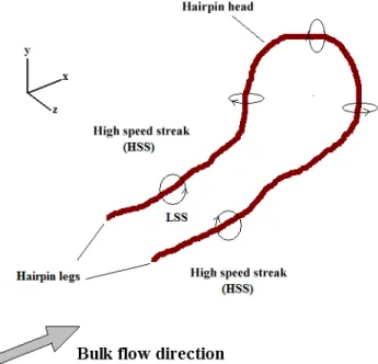
[Nakayama Y. 2000]) ………...21 Fig 2.3 Schematic of a hairpin structure in the near wall-region ……….22 Fig 2.4 Schematic of a hairpin packet structure in the near wall-region (modified from [Adrian R.J. 2000]) ………..23 Fig 2.5 Visualization of hairpin structures in the turbulent boundary layer on a flat plate at
Re 4300
m
obtained by isosurfaces of negative 2 from DNS results. The structures have been colored by wall distance [Schlatter et al. 2011] ……….23 Fig 2.6 Typical comparison of turbulence treatment strategies [Buntic et al. 2005] ……..26 Fig 2.7 Resolved and subgrid scale eddies (fluctuations) on a given mesh in the LES
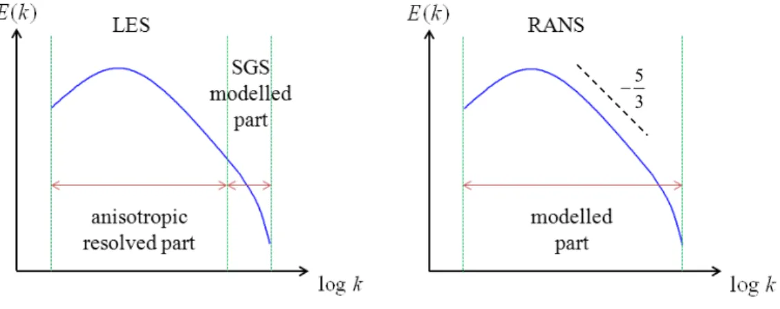
………...27 Fig 2.8 Turbulence treatment in LES vs. RANS ………..28 Fig 2.9 Turbulence treatment in VLES vs. LES method………..31 Fig 2.10 Ambiguous grid in the near wall zone inside the boundary layer (P: a point inside
B.L., : B.L. thickness, d: distance to the wall) ……….36 Fig 2.11 Turbulent flow structures (Q350) resolved by DDES turbulent treatment using unsteady 2D inflow profile in the BulbT draft tube at an overload condition …...39 Fig 3.1 Control volumes in the finite volume method used for the discretization (modified
from [OpenFOAM programmer’s guide]) ………...………47 Fig 3.2 Solution procedure for the utilized PIMPLE method………..52 Fig 3.3 A typical OpenFOAM case structure for transient DDES simulations …………...57 Fig 3.4 Speed-up curve for the BulbT draft tube flow simulation on Colosse cluster …….60
xvi
Fig 3.5 Speed-up curve for the BulbT draft tube flow simulation on Guillimin cluster …..60 Fig 4.1 Schematic of a typical turbulent velocity signal ………..65 Fig 4.2 Sketch of the hydraulic profile sections in the full-machine simulation…………..65 Fig 4.3 Final version of the draft tube geometry ……….66 Fig 4.4 Circumferential averaged-1D inlet profile obtained from full machine k
simulation at OP.4 ………...69 Fig 4.5 General Sketch on applying a transient 2D inflow profile for DDES simulation of
the draft tube using OpenFOAM ………..70 Fig 4.6 2D variation of the axial velocity u (left) and turbulent eddy viscosity Z t (right) at inlet plane from k RANS at OP.4 ………71 Fig 4.7 Delaunay triangulation at the draft tube inlet plane at one instant of time ………..71 Fig 4.8 Rotation of the 2D velocity profiles at the draft tube inlet plane for OP.4, top: radial
velocity (u ) middle: circumferential velocity ( ur ) bottom: axial velocity (u )...72 z
Fig 4.9 Power spectrum of the axial velocity signal generated by 2D rotating profile at one Eulerian probe placed at the normalized position ( /x RInlet, /y RInlet) (0.3, 0.55) ……….………..73 Fig 4.10 Schematic of the RANS (B.L.) & LES (core flow) zones at draft tube inlet plane
………...74 Fig 4.11 Function f at the draft tube inlet plane for OP.4……….75 d
Fig 4.12 Subgrid scale viscosity treatment using Smagorinsky model for OP.4 at the draft tube inlet plane………..76 Fig 4.13 Hybrid turbulent/subgrid-scale viscosity treatment for OP.4……….76 Fig 4.14 Energy spectrum of a real turbulent velocity signal (solid curve) & the white noise
signal (horizontal dashed line) ……….86 Fig 4.15 Definition of intermediate random angles, wave number vector and Fourier mode
direction ………87 Fig 4.16 Isotropic AFG fluctuation signals in axial direction with/without time-correlation before applying runner rotation and inflow anisotropy ………90 Fig 4.17 Isotropic AFG turbulent velocity fluctuation signals with time-correlation and
considering runner rotation (top: full signal, bottom: zoomed area) ………...91 Fig 4.18 Inflow AFG fluctuation field of axial velocity component at t1.2s for OP.4
(top: isometric view, bottom: side view) ………..93 Fig 4.19 Experimental RMS values of the inflow velocity fluctuations at OP.4 (LDV) [top left to bottom right: circumferential, axial, radial velocities and sketch of flow pattern observed experimentally at inlet plane (plane A)] ………...95 Fig 4.20 Multi-layer perceptron architecture designed for each azimuthal angle …………96
xvii Fig 4.21 Zonal training approach for the designed MLPR ………..97 Fig 4.22 RMS values of the fluctuations OP.4 (LDV measurements) (left: circumferential
velocity, right: radial velocity) ……….98 Fig 4.23 Learning history of the designed ANN with l 0.005 at 25 ……….98 Fig 4.24 Learning history of the ANN in the unstable region with l 0.1 at 25 …...99
Fig 4.25 Radial distribution of ANN (MLPR) predictions for the parameter radial at OP.4
(from top left to bottom right: 10 , 40 , 60 , 90 ) ……….100 Fig 4.26 Two-dimensional variation of the radial parameter obtained from ANN (MLPR)
at the inlet plane for OP.4 ………..100 Fig 4.27 Quarter of the RMS field of radial velocity fluctuations using ANN for OP.4…101 Fig 4.28 Complete RMS field of the radial velocity fluctuations predicted using ANN for
OP.4 ………101 Fig 4.29 1D circumferential-average of 2D RMS field of radial velocity fluctuations at
OP.4 ………102 Fig 4.30 1D circumferential average of 2D RMS field of the experimental velocity
fluctuations at OP.4 (top: circumferential velocity, bottom: axial velocity) ……..102 Fig 4.31 Scatter plot of the isotropic turbulent velocity fluctuations generated by the AFG method before applying rotation and scaling factors sampled at a point with the normalized position ( /x RInlet, /y RInlet) (0.3, 0.55) on the inlet plane………...103 Fig 4.32 Scatter plot of uzuy fluctuations generated by the AFG method after applying rotation and scaling factor sampled at a point with the normalized position
( /x RInlet, /y RInlet) (0.3, 0.55) on the inlet plane ……….104 Fig 4.33 Scatter plot of ux uz fluctuations generated by the AFG method after applying
rotation and scaling factor sampled at a point with the normalized position ( /x RInlet, /y RInlet) (0.3, 0.55) on the inlet plane ……….105 Fig 4.34 Scatter plot of uxuy fluctuations generated by the AFG method after applying
rotation and scaling factor sampled at a point with the normalized position ( /x RInlet, /y RInlet) (0.3, 0.55) on the inlet plane ……….106 Fig 4.35 Power spectra of turbulent velocity signals with/without artificial fluctuations
sampled at a probe positioned at ( /x RInlet, /y RInlet) (0.3, 0.55) on the inlet plane ……….107 Fig 5.1 Schematic sketch of the ERCOFTAC conical diffuser with swirling generator
[Sketched base on the geometry, used by Clausen et al. 1993] ……….112 Fig 5.2 Computational domain adopted for DDES turbulence treatment in the ERCOFTAC
xviii
Fig 5.3 Variation of the C coefficient in DNS of channel flow [Pope S. 2004] ………..116 Fig 5.4 Convergence history of the k simulation case (i.e. A-1 case in table 5.2)…...117
Fig 5.5 Normalized mean axial-velocity field on the mid-plane of the diffuser obtained from k simulation case (i.e. A-1 case in table 5.2) ………..118
Fig 5.6 Comparison of the wall-parallel (u ) and circumferential ( us ) component of mean
velocity at different sections with the experimental data for extended-cases…….119
Fig 5.7 Inflow grid reconstructed by Delaunay triangulation at S1section ………..121 Fig 5.8 2D-velocity profile extracted at S1section from extended-case simulations……122
Fig 5.9 Turbulent viscosity extracted atS1section from extended-case simulations…….123
Fig 5.10 Normalized 1D-velocity profile extracted atS1section extracted from
extended-case simulations (with k and S-A turbulence models) ………...124
Fig 5.11 Normalized 1D-velocity profile extracted atS1section extracted from extended-case simulations (with S-A turbulence model with/without wall-function)……...125
Fig 5.12 Comparison of the 1D turbulent quantity profiles atS1section obtained from the
extended-case k simulation (A-1 case in table 5.2) with experimental data (left:
turbulent dissipation rate, right: turbulent kinetic energy) ……….………...126 Fig 5.13 1D profile of turbulent viscosity atS1section coming from the selected
extended-case simulations (table 5.2) ………....127
Fig 5.14 Wall-parallel (u ) and circumferential ( us ) component of mean velocity obtained from DDES simulations of base-case using different inflow conditions (inflow
profiles coming from extended-case k , S-A simulations listed in table 5.5)...129 Fig 5.15 Axial-velocity field and separation-zone isosurface (with uz ) obtained from 0
the base-case DDES simulations listed in table 5.5 ……..………...130
Fig 5.16 Typical f function variation in the base-case DDES simulation with inflow d
profile coming from k extended-case simulation (B-1 case in table 5.5) [ fd 0 : RANS, fd 1: LES] ………....130 Fig 5.17 Variation of utotal versus yat the base-case inflow section (S1section) extracted
from various extended-case simulations ………131
Fig 5.18 Wall-parallelu and circumferential us components of mean velocity obtained from URANS simulations of the base-case indicating effect of inflow radial
velocity (the different inflow conditions for the cases are presented in table 5.6) ……….134 Fig 5.19 Variation of utotal versus yof the constructed profile at the S1section ……….136
xix Fig 5.20 Variation of v versus yt of the constructed profile at the
1
S section ………...137 Fig 5.21 Wall-parallelu and circumferential us component of the mean velocity obtained
from DDES simulations of the base-case indicating effect of inflow near-wall
treatment (cases are listed in table 5.7) ….……..………...137 Fig 5.22 Wall-parallelu and circumferential us component of mean velocity obtained from DDES simulations of the base-case (effect of tuning of the inflow near-wallv )..140 t
Fig 6.1 Basic geometry of the draft tube with its geometrical divergence angles………..144 Fig 6.2 Separation zone (blue iso-surface) in the basic geometry of the draft tube obtained
from S-A (left) and k (right) RANS simulations at BEP ………147 Fig 6.3 1D circumferential-averaged of mean velocity profiles in the conical part of the
basic geometry extracted from S-A (red) and k (black) RANS simulations at BEP……….148 Fig 6.4 Draft tube recovery coefficient (left) and swirl number (right) evolution in the
streamwise direction obtained from S-A and k RANS simulations at BEP...149 Fig 6.5 f function at the inlet of the draft tube with ‘basic geometry’ at BEP…………..150 d
Fig 6.6 Mean separation-zone (blue iso-surface) and coherent structures (Q500) obtained from DDES simulations: effect of inflow v amplification in the WZ…151 t
Fig 6.7 Draft tube recovery coefficient (left) and swirl number (right) evolution in the streamwise direction obtained from DDES simulations at BEP: effect of v t
amplification in WZ……….………...152 Fig 6.8 Mean axial velocity field on the mid-plane of the draft tube obtained from DDES
simulations at BEP: effect of inflow v amplification in WZ……….153 t
Fig 6.9 1D circumferential-averaged of mean velocity profiles in the conical part of the basic geometry extracted from DDES at BEP: effect of v amplification in WZ..154 t
Fig 6.10 Energy spectrums of the turbulent axial velocity at different axial position of the axisymmetric center line of the draft tube: effect of inflowv amplification in t
WZ………...155 Fig 6.11 Sampling-lines utilized to obtain utotal versus ygraph in the transition part...…156 Fig 6.12 Variation of utotal versus yon sampling-linesS ,1 S and2 S extracted from DDES 3
simulations: effect of inflowv amplification in the WZ………156 t
Fig 6.13 Mean separation-zone (blue iso-surface) and coherent structures (Q500) in the DDES simulations: effect of the discretization scheme of the convective term …158 Fig 6.14 Instantaneous axial velocity field on the draft tube mid-plane obtained from DDES
xx
Fig 6.15 Draft tube recovery coefficient (left) and swirl number (right) evolution in z-direction of DDES simulations at BEP: effect of the convective term discretization scheme…...159 Fig 6.16 1D circumferential-averaged of mean velocity profiles in the conical part in the
DDES simulations at BEP: effect of the convective term discretization scheme...160 Fig 6.17 Energy spectrums of the turbulent axial velocity at different positions of the axisymmetric center-line of draft tube: effect of convective term discretization scheme……….161 Fig 6.18 Variation of utotal versus yon sampling-linesS ,1 S and2 S extracted from the 3
DDES simulations: effect of the convective term discretization scheme………...162 Fig 6.19 Mean separation-zone (blue iso-surface) and coherent structures (Q500) in the
DDES simulations: grid independence test………163 Fig 6.20 Draft tube recovery coefficient (left) and swirl number (right) evolution in the
streamwise direction of the DDES simulations at BEP: grid independence test…164 Fig 6.21 Energy spectra of the turbulent axial velocity at different axial position of the
axisymmetric center-line of the draft tube: grid independence test………165 Fig 6.22 Variation of utotal versus yon the sampling-linesS ,1 S and2 S extracted from the 3
DDES simulations: grid independence test ………166 Fig 6.23 A snapshot of the generated artificial fluctuations in different spatial directions in DDES simulation of the ‘basic geometry’ using ‘2D rotating+AFG’ inflow
profile………..168 Fig 6.24 Time-evolution of the turbulent fluctuation signals in different spatial directions
adopted for DDES simulation of the ‘basic geometry’ with ‘2D rotating+AFG’
profile………..169 Fig 6.25 Coherent structures with Q350 (left) and mean separation zone (right) obtained
from DDES simulations with ‘2D rotating+AFG’ inflow profile………..170
Fig 6.26 Instantaneous flow separation obtained from DDES simulations of the ‘basic geometry’ with ‘2D rotating+AFG’ inflow profile………170
Fig 6.27 Instantaneous axial velocity field on the draft tube mid-plane (x0) extracted from DDES simulation using ‘2D rotating+AFG’ and ‘1D’ inflow profiles at
BEP……….171 Fig 6.28 Draft tube recovery coefficient (left) and swirl number (right) evolution in the streamwise direction of the DDES simulations at BEP: ‘2D’ vs. ‘1D’ profiles….172
Fig 6.29 1D circumferential-averaged of mean velocity profiles in the conical part obtained from DDES simulations at BEP: ‘2D’ vs. ‘1D’ profiles……….173
Fig 6.30 Energy spectrums of the turbulent axial velocity at different axial position of the axisymmetric center-line of the draft tube: ‘2D’ vs. ‘1D’ profiles……….174
xxi Fig 7.2 Selected operating points on the turbine efficiency curve………..179 Fig 7.3 Pressure sensor positions and LDV measurement axis………..180 Fig 7.4 PIV-measurement planes namely B1, B2, S3 and S4 [Duquesne et al. 2014-3]…181 Fig 7.5 Near-wall zone of inflow profile treatments for draft tube turbulent flow
simulations using low-Re treatments e.g. S-A and DDES………..186 Fig 7.6 2D variation of yquantity on the runner-shroud surface i.e. upstream component
of the draft tube stemmed from full machine kRANS simulations…………..187 Fig 7.7 2D variation of yquantity on the runner-hub surface i.e. upstream component of the draft tube stemmed from full machine k RANS simulations………..187 Fig 7.8 Buffer-layer velocity profile variants ………188 Fig 7.9 Turbulent viscosity in the near-wall zone of the draft tube using Reichardt model for two selected operating points i.e. OP.1 and OP.4……….189 Fig 7.10 1D inflow profiles of u and uz velocities and turbulent viscosityv at Plane A t
used for draft tube flow simulations resolving to the wall at OP.1 (left) and OP.4 (right) (solid black line: reconstructed profile, solid red line with circles: LDV measurements)……….190 Fig 7.11 1D inflow profiles of radial velocity at OP.1 (left) and OP.4 (right) at Plane A (solid black line: reconstructed profile, solid red line with circles: approximation profile)……….191 Fig 7.12 Circumferential and radial velocity inflow profile correction for OP.1 (left:
original profile, right: corrected profile based on experimental data i.e. red line)……….192 Fig 7.13 Circumferential and radial velocity inflow profile correction for OP.4 (left:
original profile, right: corrected profile based on the experimental data i.e. red line)……….193 Fig 7.14 Effect of variant inflow profiles on the mean flow obtained from k URANS
simulations at OP.1 compared to the LDV-experimental data………...196 Fig 7.15 Effect of variant inflow profiles on the mean flow obtained from S-A URANS
simulations at OP.1 compared to the LDV-experimental data………...197 Fig 7.16 Effect of variant inflow profiles on the mean flow obtained from k URANS
simulations at OP.4 compared to the LDV-experimental data………...198 Fig 7.17 Effect of variant inflow profiles on the mean flow obtained from S-A URANS
simulations at OP.4 compared to the LDV-experimental data ………..199 Fig 7.18 Mean separation zone (blue iso-surface) obtained from S-A (top) and k
(bottom) URANS simulations with inflow u-correction at OP.1……….201
Fig 7.19 Draft tube recovery coefficient evolution in the streamwise direction for different variants of the URANS simulations………202
xxii
Fig 7.20 Error measure of the velocity field between k URANS simulation results and the PIV experimental data at OP.1, plane B1 (upstream/downstream)…………...205 Fig 7.21 Error measure of the velocity field between k URANS simulation results and
the PIV experimental data at OP.4, plane B1 (upstream/downstream) …………..206 Fig 7.22 Mean streamlines for k and S-A simulations at OP.1/OP.4 on the plane B1:
downstream; (red: experimental measurements, Black: numerical simul-ation)...207 Fig 7.23 Error measure of the velocity field between S-A URANS simulation results and
the PIV experimental data at OP.1, plane B1 (upstream/downstream)……...……208 Fig 7.24 Error measure of the velocity field between S-A URANS simulation results and the PIV experimental data at OP.4, plane B1 (upstream and downstream)…..…..209 Fig 7.25 Mean streamline pattern for DDES simulations using different variants of the
‘original’ inflow profile, at OP.1 on plane B1, upstream/downstream (red: experimental measurements, black: numerical simulations)………..213 Fig 7.26 Mean flow separation zone topology obtained from DDES simulations with
different inflow profiles at OP.1……….215 Fig 7.27 f function variation extracted from DDES simulation of the draft tube with ud -corrected inflow profile at OP.1………..216 Fig 7.28 Effect of “original” inflow profile variants on the mean flow obtained from DDES simulations at OP.1 compared to the LDV-experimental data………...217 Fig 7.29 Draft tube recovery coefficient evolution in streamwise direction obtained from
DDES simulations for both operating points………..218 Fig 7.30 Effect of “original” inflow profile variants on the mean flow obtained from DDES
simulations at OP.4 compared to the LDV-experimental data………...218 Fig 7.31 Turbulent kinetic energy (k) variation at the inlet plane at OP.1………219 Fig 7.32 Effect of amplification of the turbulent viscosity in the WZ on the mean flow
obtained from DDES simulations with u -corrected inflow profile at OP.1…….221
Fig 7.33 Mean streamline pattern for DDES simulations with amplification of v t
( 10n WZ
) at OP.1 on plane B1: downstream (red: measurements, Black: simulations)……….222 Fig 7.34 Error measure of the velocity field obtained from DDES simulation results with
amplification of v in the WZ (t 10n WZ
) at OP.1 at plane B1 (upstream/ downstream)………223 Fig 7.35 Mean flow separation topology obtained from DDES simulations with turbulent
viscosity amplification in WZ applied on both hub and shroud zones at OP.1…..224 Fig 7.36 Effect of amplification of v in the WZ (t 10n
WZ
) on the draft tube recovery coefficient evolution obtained from DDES simulations at OP.1………225
xxiii Fig 7.37 Time evolution of the global draft tube coefficient ( ) for DDES simulation
applying inflow u -correction and amplification of v in the WZ (t n3) at OP.1...227 Fig 7.38 Effect of amplification of v in the WZ applied just for hub/shroud with/without t u -correction at OP.1………..227 Fig 7.39 Effect of amplification of v in the WZ applied just for hub/shroud with/without t u -correction on the mean flow separation topology at OP.1………229 7.40 Effect of amplification of inflow v in the WZ applied just for hub/shroud on the error t
measure of the velocity field with/without u -correction at plane B1 at OP.1 a) u -corrected, 3for both hub & shroudn ; b) u-corrected, 3 just for hubn , c) u -corrected, 3 just for shroudn ; d) Original velocity profile, n 3
for both hub & shroud ……….230 7.41 Coherent structures formed in the BulbT draft tube turbulent flow using DDES at
OP.1 a) Reverse-flow bubble, b) Coherent structures visualized with 2000
Q ……….231
7.42 Topology of the mean separated region for intermediate/fine girds at OP.4 visualized by iso-surface of the negative velocity ………...233 Fig 7.43 Error measure obtained from DDES simulations at OP.4 for both the intermediate (mesh B) and fine (mesh C) grids on the planes B1, B2 (upstream/ downstream)………234 Fig 7.44 Error measure obtained from DDES simulations at OP.4 for both the intermediate (mesh B) and fine (mesh C) grids on the planes S3, S4 (upstream/downstream)...235 Fig 7.45 Reverse-flow intermittency on the different slices extracted from the DDES
simulation using 1D-inflow profile at OP.4………237 Fig 7.46 Evolution of the axial velocity (top) and reverse-flow intermittency (bottom) for
two probes extracted from the DDES simulation using 1D inflow profile at OP.4……….238 Fig 7.47 Reconstruction of the uprofile for DDES simulations with unsteady 2D-inflow
profiles ………240 Fig 7.48 Circumferential-averaging of the blended 2D u-profile at OP.4 (black: averaged curve of the 2D profile, red: experimental data)……….241 Fig 7.49 Turbulent flow coherent structure anatomy resolved by Q350 coming from
DDES simulation using “2D rotating+AFG” inflow profile at OP.4……….243
Fig 7.50 Effect of different inflow profiles on the resolved coherent structures at one instant of time obtained from DDES simulations at OP.4 (colorbar: u uz ref.)…………..244
xxiv
Fig 7.51 Effect of type of the inflow profile on the mean flow obtained from DDES simulations at OP.4 compared to the LDV-experimental data………...245 Fig 7.52 Effect of inflow profile type on the draft tube recovery coefficient obtained from
DDES simulations compared to the experiment at OP.4……….………...246 Fig 7.53 Effect of inflow profile type on the time evolution of the global draft tube
coefficient ( ) obtained from DDES simulations at OP.4……….246 Fig 7.54 Topology of the mean separated region for different unsteady 2D inflow profiles at OP.4 visualized by iso-surface of the negative velocity ………247 Fig 7.55 Error measure obtained from DDES simulations using different inflow profiles at
OP.4 on planes B1, B2 (up/downstream) [ a) ( )E u x ,1D; b) ( )E u x ,2D rotating;
c)E u( )x , 2D rotating+AFG; d) ( )E u z ,1D; e) ( )E u z , 2D rotating; f) ( )E u z ,2D rotating +AFG]………248 Fig 7.56 Error measure obtained from DDES simulations using different inflow profiles at
OP.4 on planes S3 x+/x- (up/downstream) [ a) ( )
y
E u ,1D; b)E u( )y ,2D rotating; c)
( )y
E u , 2D rotating+AFG; d) ( )E u z ,1D; e) ( )E u z , 2D rotating; f) E u( )z ,2D rotating+AFG]……….249 Fig 7.57 Error measure obtained from DDES simulations using different inflow profiles at
OP.4 on the planes S4 x+/x- (upstream/downstream) [ a) ( )
y
E u ,1D; b)E u( )y ,2D rotating; c) E u( )y ,2D rotating+AFG; d) ( )E u z ,1D; e) ( )E u z , 2D rotating; f)
( )z
E u ,2D rotating+AFG]………...251 Fig 7.58 Reverse-flow intermittency on the different slices extracted from the DDES
simulations using 2D inflow profiles at OP.4……….252 Fig 7.59 Evolution of the axial velocity (left) and reverse-flow intermittency (right) at
probe A; extracted from DDES simulations using 2D inflow profiles at OP.4...253 Fig 7.60 Evolution of the axial velocity (left) and reverse-flow intermittency (right) at
probe B; extracted from DDES simulations using 2D inflow profiles at OP.4……….254 Fig 7.61 LES-content via LES IQ v obtained from DDES simulations with different
unsteady 2D inflow profiles at OP.4………...255 Fig 7.62 Energy spectra of the turbulent velocity signals obtained from DDES simulations
with different inflow profiles at different x-positions of plane B………...256
Fig 7.63 Triple view of the probe positions adopted to calculate two-point correlation (top: isometric view, bottom-left: side-view, bottom-right: front-view)……….259 Fig 7.64 Normalized two-point correlation field for the radial velocity unsteady term i.e.
†, 11
norm
extracted from DDES simulations at OP.4 with/without AFG on planes 1, 2, 3………...260
xxv Fig 7.65 Variation of the unsteady portion of the turbulent radial velocity signal †
1( )
u t in
terms of time obtained from DDES simulations with “2D rotating +AFG” inflow profile at OP.4 at two probe positions presented in table 7.8 (red: probe C, blue: probe D) ……….261 Fig 7.66 Normalized two-point correlation field for circumferential velocity unsteady term,
†, 22
norm
, extracted from DDES simulations at OP.4 with/without AFG on planes 1, 2, 3………...262 Fig 7.67 Normalized two-point correlation field for axial velocity unsteady term i.e. †,
33
norm
extracted from DDES simulations at OP.4 with/without AFG on planes 1, 2, 3………...263 Fig 7.68 Normalized two-point correlation field of radial velocity turbulent term i.e. 11norm
extracted from DDES simulations at OP.4 with/without AFG on planes 1, 2, 3………...264 Fig 7.69 Normalized two-point correlation field of circumferential velocity turbulence term i.e. 22norm extracted from DDES simulations at OP.4 with/without AFG on planes
1, 2, 3………...………265 Fig 7.70 Normalized two-point correlation field of axial velocity turbulence term i.e. 33norm
extracted from DDES simulations at OP.4 with/without AFG on planes 1, 2, 3………...266 Fig 7.71 1D plot of norm, 1, 2,3
ii i
extracted from the DDES simulation with inflow AFG at OP.4 plotted at different rows (ic=1,..,10) of the probe locations on planes 1, 2, 3………...267 Fig 7.72 Sketch of plane 1 and the hub-vortex at OP.4 indicating positions of the probes S1 to S8 utilized for the scatter plots ……..……….268 Fig 7.73 Scatter plot of the turbulent fluctuation clouds along the axial path corresponding
to the probes (S1: blue; S2: green; S3: magenta, S4: red; S5: black)……….270 Fig 7.74 Scatter plot of the turbulent fluctuation clouds along the radial path corresponding to the probes (S5: blue; S6: green; S7: red, S8: black)………...271 Fig 7.75 Flow trajectory in the proximity to the two types of the dynamical manifolds (solid red circle: initial position; hollow red circle: final position of fluid particles) …..273 Fig 7.76 Streamlines and velocity vector field of the cavity fluid flow stemmed from
kURANS simulation at Re1.5 10 6 ………276 Fig 7.77 FTLE field of the velocity field in the cavity flow case obtained from forward time
integration (T n T TC C, C 2s)………...277 Fig 7.78 FTLE field of the velocity field in the cavity flow case obtained from backward
time integration (T n T TC C, C 2s)……….278 Fig 7.79 LCS planes defined to study flow structures in the draft tube at OP.4…………279
xxvi
Fig 7.80 LCS planes defined to study reverse–flow bubble using LCS at OP.1 ………...279 Fig 7.81 Axial velocity field on the LCS planes with o o oand o
C= 0 ,45 ,90 135
from top to
bottom, at one instant of time, obtained from DDES simulation applying ‘1D’ inflow profile withu-correction and amplification of v in the WZ (t n3) at OP.1………280 Fig 7.82 FTLE field with forward-time integration (repelling LCS) on the LCS planes
with o o oand o
C= 0 ,45 ,90 135
from top to bottom, at one instant of time, at OP.1……….281 Fig 7.83 FTLE field with backward-time integration (attracting LCS) on the LCS planes
with o o oand o
C= 0 ,45 ,90 135
from top to bottom, at one instant of time, at OP.1……….282 Fig 7.84 Axial velocity field on the yz1 LCS plane obtained from DDES simulation using
‘2D rotating+AFG’ inflow condition att0.5s, at OP.4………..283
Fig 7.85 FTLE field with forward-time integration (repelling LCS) on the yz1 LCS plane calculated from DDES simulations using different inflow conditions at OP.4…..284 Fig 7.86 FTLE field with backward-time integration (attracting LCS) on the yz1 LCS plane calculated from DDES simulations using different inflow conditions at OP.4…..285 Fig 7.87 Axial velocity field on the xz1 LCS plane obtained from DDES simulation using
‘2D rotating+AFG’ inflow (top) and ‘1D’ inflow (bottom), at t0.5s, at
OP.4...285 Fig 7.88 FTLE field with forward-time integration (repelling LCS) on the xz1 LCS plane calculated from DDES simulations using different inflow conditions at OP.4 (top:
‘2D rotating+AFG’, middle: ‘2D rotating’, bottom: ‘1D’) ………...286
Fig 7.89 FTLE field with backward-time integration (attracting LCS) on the xz1 LCS plane calculated from DDES simulations using different inflow conditions at OP.4 (top:
‘2D rotating+AFG’, middle: ‘2D rotating’, bottom: ‘1D’) ………...287
Fig 7.90 Axial velocity field on the xz2 LCS plane obtained from DDES simulation using
‘2D rotating+AFG’ inflow profile, att0.5s, at OP.4 ………..288
Fig 7.91 FTLE field with forward and backward-time integrations on the xz2 LCS plane calculated from DDES simulations using different inflow conditions at OP.4 (top:
‘2D rotating+AFG’, middle: ‘2D rotating’, bottom: ‘1D’)………289
Fig 7.92 Axial velocity field on the xy1 LCS plane obtained from DDES simulation using
‘2D rotating+AFG’ inflow profile, att0.5s, at OP.4 ………..290
Fig 7.93 FTLE field with forward-time integration (repelling LCS) on the xy1 LCS plane calculated from DDES simulations using different inflow conditions at OP.4.….291 Fig 7.94 FTLE field with backward-time integration (attracting LCS) on the xy1 LCS plane
xxvii Fig 7.95 Axial velocity field on the xy2 LCS plane superimposed with repelling LCS
(black structure) and attracting LCS (cyan structure) obtained from DDES simulation using ‘2D rotating+AFG’ inflow profile, at t0.5s, at OP.4………..292 Fig 7.96 FTLE field with forward-time integration (repelling LCS) on the xy2 LCS plane
calculated from DDES simulations using different inflow conditions at OP.4.….293 Fig 7.97 FTLE field with backward-time integration (attracting LCS) on the xy2 LCS
plane calculated from DDES simulations using different inflow conditions at OP.4……….293 Fig 7.98 Axial velocity field on the xy3 LCS plane obtained from DDES simulation using
‘2D rotating+AFG’ inflow profile, at t0.5s, at OP.4………..294
Fig 7.99 FTLE field with forward-time integration (repelling LCS) on the xy3 LCS plane calculated from DDES simulations using different inflow conditions at OP.4.….294 Fig 7.100 FTLE field with backward-time integration (attracting LCS) on the xy3 LCS
plane calculated from DDES simulations using different inflow conditions at OP.4……….294 Fig B.1 Nonlinear model of a neuron………..331 Fig D.1 Computational grid for draft tube k RANS/URANS simulations (top: Full
domain draft tube mesh, bottom left: Top view of middle plane mesh intersection, bottom right: zoomed area near the hub of middle plane mesh intersection)……338
Fig D.2 Computational grid for draft tube DDES simulations. (top: Full domain draft tube
mesh, bottom left: Top view of middle plane mesh intersection, bottom right:
zoomed area near the hub of middle plane mesh intersection) ………..339 Fig G.1 Comparison of the simulation mean velocity field to the PIV experimental data
k URANS simulations, OP.1, plane B1: upstream ………..350 Fig G.2 Comparison of the simulation mean velocity field to the PIV experimental data
k URANS simulations, OP.1, plane B1: downstream………..351 Fig G.3 Comparison of the simulation mean velocity field to the PIV experimental data
k URANS simulations, OP.4, plane B1: upstream ………..351 Fig G.4 Comparison of the simulation mean velocity field to the PIV experimental data
k URANS simulations, OP.4, plane B1: downstream ……….352 Fig G.5 Comparison of the simulation mean velocity field to the PIV experimental data
k URANS simulations, OP.4, plane B2: upstream ………..352 Fig G.6 Comparison of the simulation mean velocity field to the PIV experimental data
k URANS simulations, OP.4, plane B2: downstream ……….353 Fig G.7 Comparison of the simulation mean velocity field to the PIV experimental data S-A URANS simulations, OP.1, plane B1: upstream ………353 Fig G.8 Comparison of the simulation mean velocity field to the PIV experimental data S-A URANS simulations, OP.1, plane B1: downstream………354
xxviii
Fig G.9 Comparison of the simulation mean velocity field to the PIV experimental data S-A URANS simulations, OP.4, plane B1: upstream ………355 Fig G.10 Simulation mean velocity field in the case ofu ,u inflow corrected profile S-A r
URANS simulations, OP.4, plane B1: upstream ………355 Fig G.11 Comparison of the simulation mean velocity field to the PIV experimental data
S-A URANS simulations, OP.4, plane B1: downstream ………...355 Fig G.12 Simulation mean velocity field in the case ofu ,u inflow corrected profile S-A r
URANS simulations, OP.4, plane B1: downstream………356 Fig G.13 Comparison of the simulation mean velocity field to the PIV experimental data
S-A URANS simulations, OP.4, plane B2: upstream ………356 Fig G.14 Simulation mean velocity field in the case ofu ,u inflow corrected profile S-A r
URANS simulations, OP.4, plane B2: upstream……….357 Fig G.15 Comparison of the simulation mean velocity field to the PIV experimental data
S-A URANS simulations, OP.4, plane B2: downstream ………...357 Fig G.16 Simulation mean velocity field in the case ofu ,u inflow corrected profile S-A r
URANS simulations, OP.4, plane B2: downstream ………...357 Fig G.17 Effects of v amplification on the simulation mean velocity fields DDES t
simulations, OP.1, plane B1: upstream ………..358 Fig G.18 Effects of v amplification on the simulation mean velocity fields DDES t
simulations, OP.1, plane B1: downstream ……….358 Fig G.19 Effects of v amplification with inclusion/exclusion hub/shroud on the simulation t
mean velocity fields obtained from DDES simulations, OP.1, plane B1: upstream ……….359 Fig G.20 Effects of v amplification with inclusion/exclusion hub/shroud on the simulation t
mean velocity fields obtained from DDES simulations, OP.1, plane B1: downstream ……….360 Fig G.21 Effects of mesh resolution on the simulation mean velocity fields obtained from
DDES simulations using 1D profile, OP.4, plane B1……….360 Fig G.22 Effects of mesh resolution on the simulation mean velocity fields obtained from
DDES simulations using 1D profile, OP.4, plane B2……….361 Fig G.23 Effects of mesh resolution on the simulation mean velocity fields obtained from
DDES simulations using 1D profile, OP.4, plane S3 x+……….362
Fig G.24 Effects of mesh resolution on the simulation mean velocity fields obtained from DDES simulations using 1D profile, OP.4, plane S4 x+……….363
Fig G.25 Effects of type of the inflow profile on the DDES simulation results, OP.4, plane B1: upstream ………..363
xxix Fig G.26 Effects of type of the inflow profile on the DDES simulation results, OP.4, plane B1: downstream ……….364 Fig G.27 Effects of type of the inflow profile on the DDES simulation results, OP.4, plane
B2: upstream ………..365 Fig G.28 Effects of type of the inflow profile on the DDES simulation results, OP.4, plane
B2: downstream ……….365 Fig G.29 Effects of type of the inflow profile on the DDES simulation results, OP.4, plane
S3 x+: upstream ………..366
Fig G.30 Effects of type of the inflow profile on the DDES simulation results, OP.4, plane
S3 x-: upstream ………...366
Fig G.31 Effects of type of the inflow profile on the DDES simulation results, OP.4, plane
S3 x+: downstream ……….366
Fig G.32 Effects of type of the inflow profile on the DDES simulation results, OP.4, plane
S3 x+: downstream ……….367
Fig G.33 Effects of type of the inflow profile on the DDES simulation results, OP.4, plane
S4 x+: upstream ………..……367
Fig G.34 Effects of type of the inflow profile on the DDES simulation results, OP.4, plane
S4 x-: upstream ………...368
Fig G.35 Effects of type of the inflow profile on the DDES simulation results, OP.4, plane
S4 x+: downstream ……….368
Fig G.36 Effects of type of the inflow profile on the DDES simulation results, OP.4, plane
S4 x-: downstream ………..369
xxxi
Nomenclature
Latin Symbols
z
A Cross-section area of each section perpendicular to z direction [m2]
Inlet
A Cross-section area of the inlet [m2]
N
a Off-diagonal coefficients in the discretized transport equation [-]
P
a Diagonal coefficient in the discretized transport equation [-]
ij
a Amplitude tensor in Cholesky decomposition [m.s-1]
B Constant in the non-dimensional relation of log-layer [-]
ij
b Coefficients in linear combination of AFG signal [m.s-1]
p i
b Bias added for each neuron [-]
DES
C Detached eddy simulation model constant (0.65) [-]
S
C Smagorinsky constant (0.1 0.2 ) [-]
C Empirical Coefficient in eddy-viscosity model [-]
v
c Constant in the LES-index formulation [kg.m-3]
D Diameter of hydro-turbines [m]
D Dt Material (substantial) derivative ( t uj xj) [s-1] d Wall distance in Spalart-Allmaras model [m]
d DES length scale [m] ( )s
E k Energy in the modified von Karman spectrum [m3.s-2]
()
E Difference (error) measure between PIV-2D field and numerical counterpart [-] F Mass flux [kg.s-1]
d
xxxii
ij
f Uncorrelated random fields [-]
c f Cut-off frequency [s-1] g Acceleration of gravity [m.s-2] H Water head [m] V k Von-Karman constant (0.41) [-]
k Turbulent kinetic energy per unit mass [m2.s-2]
n j
k Wave number vector in Davidson-Billson AFG method [m-1]
1
k Smallest wave number in the turbulence spectrum [m-1]
e
k Most energetic eddy wave number in the turbulence spectrum [m-1]
max
k Highest wave number in the turbulence spectrum [m-1]
s
k Wave number in the modified von Karman spectrum [m-1]
k Intermediate wave number in the modified von Karman spectrum [m-1]
t
L Turbulent length scale [m]
v
LES IQ LES index indicating LES content of the simulation [-] l Largest length scale in the flow field [m]
m
l Mixing length scale [m]
m Time step number in time digital filtering [-] m Mass flow rate [kg.s-1]
N Runner rotation speed [rev.s-1]
s
n Specific speed [-]
v
n Constant in LES index (=0.53) [-]
n Unit vector pointing outward of a surface [-] n Iteration number in ANN learning [-]
C
n Time factor in the cavity test case [-] 11
xxxiii
e
N Number of eddies at inlet plane in SEM [-]
K
N Number of modes in Kraichnan AFG method [-]
f
N Number of Fourier modes in Davidson-Billson AFG method [-]
C
N Number of cores hired for parallel computing [-] p Static pressure [N.m-2]
P Total pressure [N.m-2]
D
p Scaling factor of most energetic eddy to the largest eddies [-]
z
p Average pressure of the four azimuthal mean pressures (sensors) [N.m-2]
Inlet
p Average pressure of the four azimuthal mean pressures at inlet [N.m-2] ,ij
p Hessian of pressure [N.m-4] q Fluid kinetic energy [N.m-2]
Q Second invariant of velocity gradient tensor
f
Q Flow rate [m3/s]
r Radial component in cylindrical coordinate system [m]
P
R RHS of the discretized transport equation [-]
d
r An intermediate parameter defined in DDES [-]
i
r Random white-noise signal [-]
Re Reynolds number [-]
Re Reynolds number based on momentum thickness of B.L. [-]
Inlet
R Radius of the draft tube cone at the inlet plane [m]
B
R Radius of the section B after the hub [m]
w
S Swirl number [-]
S Source term in the general transport equation [-] ,
S S Strain rate tensor (symmetric part of velocity gradient tensor) [s-1]
t
xxxiv
T Time interval FTLE [s]
u Friction velocity [m.s-1] U Velocity vector [m.s-1] , i j U Velocity gradient [s-1] . ref u Reference velocity [m.s-1] i
u Mean velocity component (i=1, 2, 3 corresponding to x,y,z directions) [m.s-1]
u Non-dimensionalized velocity in the wall units [-]
i
u Turbulent velocity signal [m.s-1]
m i
u Mean velocity in RANS and URANS [m.s-1]
i
u Coherent part of turbulent velocity signal [m.s-1]
l i
u Low frequency fluctuating part of the turbulent velocity signal [m.s-1] †( )
i
u t Unsteady part of the velocity signal in the Reynolds triple decomposition [m.s-1]
i
u High frequency fluctuating part of the turbulent velocity signal [m.s-1]
s
u Sub-grid scale (residual) fluctuations in LES [m.s-1]
s
u Velocity component parallel to the wall in ERCOFTAC diffuser [m.s-1] u Resolved velocity in LES [m.s-1]
x
u Lateral component of velocity defined in PIV-planes [m.s-1]
y
u Vertical component of velocity defined in PIV-planes [m.s-1]
z
u Streamwise component of velocity defined in PIV-planes [m.s-1] ˆn
u Modified von Karman spectrum amplitude [m.s-1]
u Circumferential velocity fluctuation [m.s-1]
z
u Axial velocity fluctuation [m.s-1]
r
u Radial velocity fluctuation [m.s-1]
P
xxxv
p i
v Activation potential of neuron i in ANN [-]
,
p i j
w Synaptic weights in an ANN inter-connection [-] x Position vector in flow computational domain [m] ( , )x y Position at the draft tube inlet plane
p j
x Neuron input in the neuron model [-]
y Non-dimensionalized distance from the wall in the wall units [-] y Distance from the wall [m]
p j
y Neuron output in the neuron model [-] ˆI
z Separation distance in the definition of two-point correlation [m]
Greek Symbols
Fluid density [kg.m-3]
Dynamic viscosity [Pa.s]
Turbulent eddy dissipation [m2.s-3]
ji
Sign on vortex j in i dir. (independent random steps of values +1 or -1) [-] Vorticity [s-1]
Dimensionless power coefficient [-]
D
Diffusion Coefficient [m2.s-1]
FTLE
FTLE (or equivalently DLE) field [s-1]
Hydro-turbine efficiency [-]
l
Learning rate in ANN learning process [-] Recovery coefficient [-]
Experimental recovery coefficient [-] max
C G
xxxvi
ANN
ANN activation function [-] s+1
i
Local gradient at neuron i in layer (s +1) [-]
pattern
2D pattern of the inflow radial velocity field [-]
L Loss coefficient [-] , j k Discrete wavelets [-] n
Phase shift in Davidson-Billson AFG method [-]
.
Kol
Kolmogorov length scale [m]
j i
Random amplitude in the Kraichnan AFG method [m.s-1]
WZ
Amplification factor of the turbulent viscosity in the near-wall zone [-]
, ,
i j k
Wavelet coefficients [m.s-1]
Runner
Runner opening angle [-]
radial
Scaling parameter in ANN-based radial velocity prediction [-]
1
s
Relative amplitude of the radial to axial fluctuations [-]
2
s
Relative amplitude of the circumferential to axial fluctuations [-]
r scaling
Scaling factor of the fluctuations in radial direction [-]
scaling
Scaling factor of the fluctuations in circumferential direction [-]
z scaling
Scaling factor of the fluctuations in axial direction [-]
j i
Random amplitude in the Kraichnan AFG method [m.s-1]
j k
Wave number vector component in the Kraichnan AFG method [m-1]
j k
Phase vector component in the Kraichnan AFG method [s-1]
Boundary layer thickness [m]
v
Viscous length scale [m]
ij
Kronecker delta [-]
Intermittency
xxxvii
Distance between stretched points in time interval T in the FTLE [m]
n i
Fourier mode direction in Davidson-Billson AFG method [-]
W
Wall shear stress [N.m-2]
ij
Reynolds stress tensor (u ui j) [kg.m-1.s-2]
S ij
Sub-grid scale (SGS) stress tensor [kg.m-1.s-2]
v Kinematic viscosity [s-1.m2] (v )
t
v Turbulent eddy viscosity [s-1.m2]
v Modified turbulent viscosity in SA model [s-1.m2]
SGS
v Sub-grid scale turbulent viscosity [s-1.m2]
DES
v DES turbulent viscosity [s-1.m2]
.
eff
v Effective viscosity in the LES-index formulation [s-1.m2]
num
v Numerical viscosity in the LES-index formulation [s-1.m2]
Azimuthal angle component in cylindrical coordinate system [-]
m
Momentum thickness [m]
C
Cutting-angle of the planes to study separation bubble [-]
2
Negative Eigen value of the corrected Hessian of pressure tensor [-]
Passive scalar quantity [-] Diffusion coefficient [-]
t
Time step [s]
C G
Finite-time Cauchy-Green deformation tensor [-] Grid spacing measure [m-1]
f
Filter width in LES method [m-1]
Coefficient in the time digital filtering [-]
Coefficient in the time digital filtering [-]