Centre de Recherche en économie de l’Environnement, de l’Agroalimentaire, des Transports et de l’Énergie Center for Research on the economics of the Environment, Agri‐food, Transports and Energy _______________________
Barla: Professor at the Department of Economics, Université Laval and CREATE, Pavillon J.‐A.‐DeSève, 1025 avenue des Sciences‐
Humaines, Québec (Québec) Canada G1V 0A6, [email protected]. Herrmann: Professor at the Department of Economics, Université Laval and CREATE Ordás Criado: Professor at the Department of Economics, Université Laval and CREATE Miranda‐Moreno: Professor at the Department of Civil Engineering and Applied Mechanics, McGill University Les cahiers de recherche du CREATE ne font pas l’objet d’un processus d’évaluation par les pairs/CREATE working papers do not undergo a peer review process. ISSN 1927‐5544
Are Gasoline Demand Elasticities Different across Cities?
Philippe Barla
Markus Herrmann
Carlos Ordás Criado
Luis F. Miranda‐Moreno
Cahier de recherche/Working Paper 2015‐4
Septembre/September 2015
Abstract: In this paper, we examine the heterogeneity in gasoline demand price and income
elasticities across 40 cities in the province of Quebec Canada using quarterly data over the 2004 to 2009 period. We reject the hypothesis of identical elasticities across markets. However, the range of values for the price elasticity, between -0.65 and -0.14, is relatively narrow and confirms that the demand for gasoline is price inelastic. We find evidence that the average price and income elasticity is somewhat larger in markets with public transportation. Furthermore, these markets experience a strong declining trend in gasoline use per capita.
Keywords: Gasoline demand, price and income elasticities, random coefficient model, peak car hypothesis
Classification JEL: C33, D12, Q41
Acknowledgments: we thank Pierre Tremblay and Nadia Desfossés from the Quebec Ministry of
Transport for their useful suggestions. We also thank the seminar participants to the 2014 ITEA Conference in Toulouse for their helpful remarks. We acknowledge the financial support from the Ministère des transports du Québec. All the views expressed in this paper are however solely ours.
2
1. Introduction
This paper investigates how gasoline demand varies across markets. In particular, we compare the responsiveness of gasoline demand to price and income in two types of markets namely large urban cities with a good public transportation system and small to median cities that rely almost exclusively on private vehicles. First, we show, theoretically, that the demand for gasoline in a city with a public transportation system is not necessarily more price elastic than the demand in a city without the presence of this substitute. Second, we carry out an empirical analysis using quarterly data on gasoline sales in 40 municipalities and metropolitan areas in the province of Quebec (Canada) over the 2004-2009 period. For the two market groups, we estimate a demand function that depends upon the price of gasoline, the level of disposable income, seasonal effects and a random market specific effect. Furthermore, we allow some coefficients to be random in order to account for within group heterogeneity. Our empirical results show that the price and income elasticities are statistically different across markets but with a range of values that is relatively limited. We also find that the average price elasticity in cities with public transit is larger than in cities without (0.22 versus 0.12). However, the most striking result is the sharp negative trend in per capita gasoline demand in large urban cities with public transit. Indeed, in these markets, we obtain an average annual reduction of 2% (all else being equal) which provides additional evidence that the use of cars in large cities may be stagnating or even declining
(Goodwin and Van Dender, 2013).
There is an important body of literature on gasoline demand but the number of studies testing for variations in gasoline elasticities across markets is rather smaller. Some of the existing studies compare elasticities values across countries (Dahl, 1982; Baltagi and Griffin, 1983; 1997; Brons
3
et al 2008) finding few systemic variations. Some recent studies compare the elasticity across time periods and find evidence that the price elasticity of gasoline in the US has declined over time (Small and Van Dender, 2007; Hughes et al. 2008). This decline would be caused by urban sprawl and improved standard of living which would have increased automobile dependency.
Another strand of the literature uses micro level data to study heterogeneity in gasoline demand elasticities across households. These analyses either directly estimate household gasoline demand (Wadud et al. 2009, Wadud et al. 2010) or they study one of its main determinants namely vehicle miles traveled (Gillingham, 2013, Wang and Chen, 2014). Overall, these studies confirm the existence of heterogeneity across households but provide, so far, little consensus on its pattern. For example, while some studies find that price elasticity decreases with the level of household income (West and Williams, 2004, Wadud et al. 2009, Wadud et al. 2010) others find the opposite (Kayser, 2000, Gillinghma, 2013). A U-shaped relationship is derived by West (2004) and an inverted U-shape by Wand and Chen (2014). Some researchers find that the price elasticity is more important in urban settings (Wadud et al. 2009, Wadud et al., 2010) but others find the opposite (Gillingham, 2013). The evidence on income elasticity also varies greatly across studies. For the US, Wadud et al. (2009) finds lower price elasticity in rural regions (-0.17) than in urban areas (-0.3).
Compared to a country (or state) level analysis, using city level data offer more opportunities to analyze demand in differentiated environments. Household level data allows a very precise analysis of demand heterogeneity but these data are not always available. Moreover, they are often either cross sections or short panels thereby making the identification of the price effect somewhat more difficult. Obviously, using city level data has its own shortcomings especially the risk that gasoline sales in a city (particularly in small ones) do not necessarily reflect gasoline
4
demand of its residents adequately. Indeed, residents may buy gasoline elsewhere and non-residents may inflate city sales.
To our knowledge, our study is amongst the first studies to use gasoline data at city level. Recently however, Levin, Lewis and Wolak (2013) have used daily expenditure data and prices to analyse the demand for gasoline in 243 U.S. metropolitan areas from 2006 to 2009. While, the main focus of their analysis is on the impact of using high frequency data, they do however also report some results on variations in price elasticities across cities. They find that almost all cities have gasoline price elasticities ranging from -0.35 to -0.45. They also find that more densely populated cities, those with more low income households or a higher share of commuters using subways or rails have somewhat more elastic demand. Besides using data from a different country, our study is different as it compares cities of very different size ranging from large metropolitan areas to small cities with a few thousands residents.
In section 2, we present a very simple theoretical model to illustrate the potential impact of public transportation on gasoline demand at the city level. In section 3, we describe the data and the criteria used to classify cities. The empirical specification and results are presented in section 4. We conclude in section 5.
2. The impact of public transportation on gasoline demand
A distinguishing feature of many large cities is the supply of public transportation, a substitute to private vehicles. It may be tempting to anticipate that markets with public transportation should necessarily exhibit greater price elasticity of gasoline demand. In fact, the very simple model below illustrates that this initial intuition may not necessarily be adequate.
5
ln 1 ln (1)
with a composite good, the distance travelled by cars and the distance travelled by
public transit (e.g. bus or light rail). For the sake of simplicity, cars and public transit are assumed to be perfect substitutes. Thus, the mode choice only depends upon the comparison of the generalized travel costs. For the automobile, the cost per unit of distance is given by:
(2)
The first term is the fuel cost per unit of distance with the fuel consumption rate per unit of
distance and the price of gasoline. comprises the other monetary costs such as insurance and
vehicle depreciation. The third term is the cost of travel time which depends upon the value of
time evaluated by the individual hourly wage and the average speed of car travel .
Similarly, the public transit generalized cost is
(3)
with the monetary costs of using public transit. To make the analysis interesting, we assume
that and so that depending upon some individuals find it cost efficient
to travel by transit and others by car. Specifically, individuals with
∗ (4)
travel by car ( 0 and 0 . For those individuals, the distance travelled is given
by maximizing (1) under the budget constraint
6
with Z the exogenous number of hours worked per day. Individual i’s gasoline demand is
. (6)
Her gasoline price elasticity is
, (7)
which is decreasing in .1 Her income elasticity
, (8)
is also decreasing in .
Assuming a continuum of individuals with an income density distribution over the support
, with <w* and >w*, the aggregate gasoline demand in a market with public transit
(referred with superscript T for Transit) is given by
,
∗ (9)
It can easily be shown using Leibniz integral rule that the aggregate demand price elasticity is
, , ,
, ∗
∗ ∗ ∗ ∗ ,
(10)
The first term is a weighted average of the individual demand elasticity of those travelling by cars. The weight is given by the individual share in the aggregate demand. The elasticity is
7
however higher as some car users transfer to public transit following the price increase. This
shift is measured by the second term in (10) with ∗ , measuring the elasticity of ∗
with respect to .
In a city with no public transit system (referred by superscript NT for No Transit), the only available mode is the automobile so that the aggregate demand is given by:
, (11)
and the elasticity is:
, , , (12)
Comparing (10) and (12), it can be easily shown that the first term in (10) is smaller than (12) if
the price elasticity is declining with the level of income.2 The intuition is clear: transit subtracts
from the gasoline demand low-income individuals that have higher , . So it is very well
possible that, if the second term in (10) is small, we have , , i.e. the price elasticity
is smaller in the city with public transit.
As an example, suppose that there are only two groups of individuals: group 1 has N1 individuals
with hourly wage and group 2, N2 individuals with wage . In this case, in a city without
public transit, the gasoline demand price elasticity is a weighted average of the two groups
elasticity , , , . With public transit, only group 2
individuals have a positive demand for gasoline so that the demand elasticity is , , .
8
It follows in this case that, we end up with a gasoline demand which is more price elastic in the
market without the substitute, i.e. , , .
Obviously, the opposite may also occur. In fact, three aspects are required for observing lower price elasticity in markets with public transit: i) transit is chosen by low income individuals (i.e. it is an inferior good), ii) these individuals have higher elasticities and iii) modal shift is low
following a gasoline price increase. While public transportation is often used as an example of an inferior good, the empirical evidence is mixed. Holmgren (2007) reviews 22 studies and reports income elasticities of transit demand ranging from -0.82 to 1.18 with a mean at 0.17. A review of the literature by Paulley et al. (2006) provides more conclusive evidence with transit being an inferior good when the impact of income on car ownership is properly taken into account. They report income elasticities ranging from -0.5 to -1.
As already mentioned in the introduction, the empirical evidence concerning point ii) are mixed. In fact, some empirical studies (Kayser, 2000, Gillingham, 2013) find that low income
households have lower price and income elasticities. One explanation is that these households have very little latitude to reduce gasoline consumption as they already only use their cars for
bare necessities. It is easy to modify our model to include a minimum level of travel .3 In
such a setting, low income households may end up having a demand for gasoline that is perfectly inelastic. Also, higher income households have more options to adjust to higher prices. They can reduce discretionary travels or switch to air travel for long distance trips. Moreover, high income households often have several cars thereby allowing reductions in gasoline consumption by increasing the use of the most efficient vehicles.
9
Concerning the modal transfer due to a change in gasoline price, the empirical evidence on the related concept of transit demand elasticity with respect to gasoline price indicates some mode shifting. For example, Lane (2011) obtained a long term elasticity of 0.4 for bus and 0.8 for rail using data for 33 metropolitan areas in the US. Even if these elasticties are high, the impact on gasoline demand may still be quite low when the initial market share of transit is low.
In conclusion, it is ambiguous based on economic theory whether cities with transit should exhibit higher or lower price and income elasticities. We therefore turn next to an empirical investigation of this question.
3. The data
Data on quantities of gasoline sold by market are provided by The Kent Group, a private
company that collects data through on-site visits at about 7000 gasoline stations in more than 300 markets in Canada. Our sample includes quarterly volume from 2004 to 2009 in 40 markets
located in the province of Quebec (Canada).4 Most markets correspond to either a municipality
or a metropolitan area. There is however one exception; the largest metropolitan area in the
province, Montreal, is divided into 4 markets.5 The average quarterly price of gasoline (regular
only) is obtained through the Régie de l’Énergie, a public regulating organization. The price data are however only available by administrative regions, a territorial division that is usually larger than the city limits. We expect however that the correlation between the regional and market prices is high. Moreover, the price variability across markets is marginal relative to the temporal
4 All the grades of gasoline (regular, premium, premium plus) are aggregated. Diesel is not included but diesel light duty vehicles represent less than 1% of the vehicle fleet in Quebec. The data initially included 43 markets but we have aggregated three markets with other existing markets in the Montreal area.
10
price changes. The socio-demographic market characteristics including city population and per capita personal income are provided by Institut de la Statistique du Québec and Statistics
Canada. Unfortunately, these variables are only available on an annual basis thereby reducing
their variability.
Table 1 provides some descriptive statistics with markets being classified in two groups based on the importance of public transportation. Specifically, we regroup all the markets where at least 10% of workers commute by public transit based on the 2006 census data. This group includes seven markets which are all located in the province’s three largest metropolitan areas. We refer to this group as HTransit for high transit markets. The remaining 33 markets include
municipalities with population ranging from 3,000 to 400,000. In this group, the share of
workers commuting by transit ranges from 0 to 6.4%. We refer to this group as LTransit for low transit markets. Figure 1 illustrates the changes in the average gasoline sale per capita in both market groups over the 2004-2009 period.
We observe that the HTransit group is characterized by gasoline sales per capita that are 30% lower and a smaller number of vehicles per capita. All the markets in the transit group have experienced a statistically significant negative trend in per capita gasoline sales over the 2004 and
2009 period.6 For the LTransit group, 16 markets experience a positive trend, 10 a negative one
and the remaining 7 markets no significant trend. The average income in the Htransit group is 14% higher and the average population density is close to six times larger than in the LTransit
group.7 There is little difference in the average gasoline price across the two groups. In the
6 For each market, we regress the log of per capita sales on a trend.
7 Some markets in the transit group have an average population density that is relatively low. Still, these markets have a highly dense urban core that sustains a public transit system.
11
LTransit group, we observe a very wide range in gasoline per capita. Some markets have very
large sales per capita because of substantial external demands. This is the case for markets located along highways and cities with touristic attractions. Finally, Figure 2 illustrates the changes in the average gasoline real price over the 2004 to 2009 period. We observe a steady increase from 2004 to 2008 followed by a severe drop following the financial crisis.
Table 1. Descriptive statistics by market groups (mean and [min./max.])
HTransit LTransit Gasoline sale per capita (litres) 221
[142/296]
319 [114/1722]
Average annual variation in gasoline sale per capita (%) -2.2 [-3.9/-0.52]
1.12 [-2.4/6.9]
Real gasoline price
(cents per litres - $ of 2002)
93 [71/126]
93 [75/125]
Real per capita personal annual income (2002 $) 23,129 [19,587/28,111] 20,231 [15,917/25,331] Population (in 1000) 595 [240/1 307] 49 [3/377] Population density 1,370 [198/4,483] 235 [7/847]
Share of worker commuting with transit in 2006 (%) 18.8 [11.2/37.6]
1.5 [0/6.3]
Number of vehicle per capita 0.52
[0.36/0.6]
0.58 [0.39/0.92]
12
Figure 1. Average Per Capita Gasoline Consumption for HTransit and LTransit markets (liters per quarter)
Figure 2. Real regular gasoline price in the Montreal market
20 0 22 0 24 0 26 0 28 0 G a so lin e Sa le s Pe r Ca p it a ( lit e rs/ q u a rt e r) 20 04 q1 20 04 q3 20 05 q1 20 05 q3 20 06 q1 20 06 q3 20 07 q1 20 07 q3 20 08 q1 20 08 q3 20 09 q1 20 09 q3 LTransit HTransit 80 90 10 0 11 0 12 0 13 0 R e g u la r g a so lin e p ri c e (ce n ts p e r l ite r, C $ 2 0 0 2 ) 20 04 q1 20 04 q3 20 05 q1 20 05 q3 20 06 q1 20 06 q3 20 07 q1 20 07 q3 20 08 q1 20 08 q3 20 09 q1 20 09 q3
13
4. The empirical analysis and results
We start the empirical analysis by comparing a restricted model that imposes the same slope parameters for all markets with an unrestricted model that allows all coefficients to be market
specific. Specifically, the unrestricted model has the following structure:8
, , , ∑ ,
(13)
where , is the quantity of gasoline per capita sold in market m at time t, , is the
average gasoline price and , the average per capita personal income. We control for the
time trend and also add a dummy to control for the possible impact of the 2008 financial crisis (Crisis is set to one starting in 2008Q3). Indeed, as illustrated in Figure 1, the price of gasoline dropped by 35% in 2008Q3. While the province of Quebec was initially spared from the economic downturn in the U.S. (i.e. Inc continued to grow), it cannot be excluded that the economic uncertainty led households and business to become more prudent and modify their
gasoline consumption. are three dummy variables to control for quarterly changes in , .
The parameters , , , are allowed to vary by markets. , is the error term.
The restricted model imposes that all the parameters are identical across markets (e.g.
. . ). The intercepts are however allowed to vary by markets to control for difference in the
average level of gasoline consumption. We compared a fixed effects ( are fixed parameters to
be estimated) and a random effect model ( are random draws from a Normal distribution).
14
Both the restricted and unrestricted specifications are static models. In fact, our time series dimension is too short (5 years) to properly estimate a dynamic model. Static models are traditionally viewed as measuring medium term effects with elasticities estimates that are
comprised between the short- and long-term effects measured with dynamic models.9
Table 2 reports the results for the restricted fixed and random effects models. The results obtained are very close. In fact, a Hausman test confirms that the random effects specification should be preferred. The price elasticity is low and the income elasticity is is not statistically significant. Note however that the income coefficient becomes significant and remains around 0.3 when the trend variable is excluded (these two variables are highly correlated). The model only explains 14% of the within market variability.
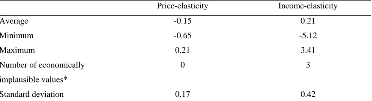
We do not report here the unrestricted estimates as the number of coefficients is very large. Instead, Table 3 reports some descriptive statistics and Figure 2 shows the kernel density of the estimated price and income elasticities values. 35 out of the 40 markets provide negative price elasticities and 9 are statistically significant at 10%. For the 5 markets that have positive price elasticity none is statistically significant. Overall however, the gasoline demand appears to be price inelastic in all markets. The range of statistically significant price elasticity is between -0.14 and -0.65. The income elasticities values are more instable. They are positive and statistically significant for 7 markets and negative and statistically significant for 3 markets.
9 Note however that in a cointegration framework, the static specification is used to measure the long term relationships. In our setting with a short panel short, it is however unlikely that our elasticities capture all the long term demand adjustment processes such as, for example, the fleet replacement.
15 Table 2. Restricted fixed and random effects model
Fixed effects Random Effects -0.133 -0.135 (0.049)*** (0.05)*** 0.281 0.244 (0.131) (0.129) Trend -0.0003 (0.0012) 0.0005 (0.001) Crisis -0.007 -0.008 (0.012) (0.017) Q1 -0.016 -0.16 (0.007)** (0.007)*** Q2 -0.003 -0.002 (0.008) (0.008) Q3 0.06 0.06 (0.007)*** (0.007)*** Q4 Reference Reference Constant 3.40 3.77 (1.33)** (1.31)*** R-sq within 0.14 0.14 N 953 953 * p<0.1; ** p<0.05; *** p<0.01 In parenthesis, robust standard deviation
A Chow test for the equality of slope coefficients across markets clearly rejects the hypothesis of
homogeneity.10 The unrestricted model provides however economically implausible results for
some markets. This may be caused by unobservable market-specific idiosyncrasy and the limited number of time period which make the estimation imprecise. This is the same type of trade-off between accounting for heterogeneity and sample size experienced by Baltagi and Griffin (1997)
16
in estimating gasoline demand in OECD countries. As a compromise, we proceed with the estimation of a model that account for some heterogeneity while still imposing some structure.
Table 3. Summary statistics for the elasticities estimated by the unrestricted model
Price-elasticity Income-elasticity Average -0.15 0.21 Minimum -0.65 -5.12 Maximum 0.21 3.41 Number of economically implausible values* 0 3 Standard deviation 0.17 0.42
* For the price elasticity a positive and statistically significant value is considered economically implausible. For the income elasticity, the value should be negative and statistically significant.
Figure 2. Kernel density based on parameters estimated in the unrestricted model
Specifically, we estimate separate models for the two market groups identified above namely
HTransit and LTransit as the preliminary evidence discussed in section 3 clearly point to
differences between these two groups. Furthermore, to better account for heterogeneity, we also allow for some parameters to be random. Specifically, we estimate for both market group
gr=HTransit, LTransit the following model:
0 1 2 3 kde n s it y e_ p -.6 -.4 -.2 0 .2
Price Elasticity Values
0 .2 .4 .6 kd e n sit y e _ y -6 -4 -2 0 2 4
17
, , ,
1 2 3 , with (13)
With this specification, the average price elasticity in the HTransit group is given by .
However, it is allowed to vary across markets through the random term , which is assumed to
be i.i.d. normal with zero mean and variance .11 Once these parameters are estimated, it is
possible to compute the best linear unbiased predictions of the random effects and thereby derive
market specific impacts (Bates and Pinheiro, 1998).12 Note that we have the same structure for
the other parameters except for those associated with Q1, Q2 and Crisis which are assumed fixed
parameters.13 is the market specific random effect.
The results are presented in Table 4. The average price elasticity is about twice as large as in markets with significant transit at -0.22 versus -0.12. This is in line with the results obtained by Levine, Lewis and Wolak (2013). In HTransit markets, we do not find any significant
heterogeneity in this parameter not statistically significant) while in LTransit,
the price elasticity varies between -0.27 and -0.05 across markets. The average income elasticity in HTransit is around 0.7 and does not exhibit significant heterogeneity. In LTransit, we do not find any significant effect of Inc. This seems once again linked to the correlation between the trend and the variable Inc. Average per capita gasoline consumption has been declining at an average rate of 0.5% per quarter in HTransit markets all else being equal. The range of decline across these markets is between 0.2% and 1%. In LTransit markets, the average trend is positive at 0.4% per quarter with significant heterogeneity across markets (between -0.4% and +1.7%).
11 This parameter is obviously also group specific.
12 A market specific impact is obtained as the sum of the average effect plus the prediction for the random term. 13 When all the coefficients are assumed random, the model becomes too complex to be estimated.
18
The financial crisis is associated with a significant decline of about 5.4% in HTransit markets while the impact is not statistically significant in LTransit. Moreover, we find that if this variable is excluded, the average price elasticity in HTransit is biased downward at -0.09. We observe very different seasonal patterns. High transit markets sales per capita decline by an average of 4% during the summer months. At the same period, sales per capita are increasing by 8.5% LTransit. There is also significant seasonal heterogeneity across markets within groups (the overall range is between -7% and +32%). These results are therefore consistent with a demand transfer across regions due to tourism and other summer specific activities.
Several alternative specifications were tested in order to assess the robustness of the results. First, the price elasticity increases at -0.3 if we use a criterion of 15% instead of 10% for defining
HTransit. Inversely, it is reduced to -0.16 with a 6% cut-off point. For the Ltransit market, the
results are very similar if we eliminate markets with a high level of external demand. The price elasticity results are also very similar if the estimation is carried over only for the data before the financial crisis (2004 to 2008Q2). We have to mention however that the income elasticity estimate and trend are much more unstable and become not statistically or economically meaningful for several specifications. This instability is likely due to the lack of variability in this variable (recall it varies only annually), the short time period of our data and the difficulty to disentangle the impact of these two variables.
19 Table 4. Results of the random coefficient models
HTransit LTransit -0.223 -0.125 (0.062)*** (0.032)*** 0.697 -0.099 (0.287)** (0.169) Trend -0.005 0.004 (0.001)*** (0.002)** CRISIS -0.054 -0.003 (0.021)** (0.013) Q1 -0.032 -0.008 (0.004)*** (0.008) Q2 -0.019 -0.004 (0.006)*** (0.006) Q3 -0.043 0.085 (0.012)*** (0.016)*** Constant -0.497 7.126 (3.096) (1.650)*** 0.008 0.061 (0.105) (0.019)*** 0.000 0.012 (0.000) (0.070) 0.002 0.050 (0.0009)*** (0.000)*** 3 0.023 0.091 (0.011)*** (0.013)*** 0.131 0.365 (0.108)** (0.249)*** 0.033 0.045 (0.007)*** (0.004)*** N 168 785
(Robust Std. Err. Adjusted for market clusters) * p<0.1; ** p<0.05; *** p<0.01
20
5. Conclusions
In this paper, we examine how price and income responsiveness of gasoline demand vary across cities in the province of Quebec (Canada). We are especially interested in the impact of public transit. Theoretically, we illustrate that observed price and income elasticity could be either higher or lower in cities with public transportation, a substitute for private car. Our empirical results indicate that the price elasticity is about doubled at -0.2 in markets with significant transit supply compared to market without. The income elasticity is around 0.7 in high transit markets while it does not appear to be statistically significant in low transit markets. These latter results should however be considered with caution as data limitations probably affect the estimation of the effect of income. The other distinguishing feature of high transit markets is the negative trend with an average annual decline in gasoline consumption close to 2% in large urban markets. The investments in public transportation, the ageing of the population, the improvements in fuel economy, congestion issues, the reduction in automobile dependency in young people but also the 2008 crisis could be some the driving factors behind this trend. The evidence we have provided here can be added to the limited but growing evidence of a peak in car use in developed countries (see Goodwin and Van Dender, 2013).
The main shortcomings of our analysis are the following. Our panel is short making the estimation of a dynamic model perilous and making it difficult to identify the income effect. Furthermore, we certainly do not measure the complete long term impacts of price and income variations. Finally, some of our results could be contaminated by the impact of the financial meltdown of 2008 even though we have tried to control for this event.
21
References
Baltagi, B. H. and Griffin, J.M. (1983) Gasoline Demand in the OECD: An Application of Pooling and Testing Procedures, European Economic Review, Vol. 22, Issue 2, pp. 117-137. Baltagi, B. H. and Griffin, J.M. (1997) Pooled estimators vs. their heterogenous counterparts in
the context of dynamic demand for gasoline, Journal of Econometrics, 77, pp. 303-327.
Basso L. and Oum, T.H. (2007) Automobile fuel demand: A critical Assessment of empirical
methodology, Transport Reviews, Vol. 27, no. 4, pp. 449-484.
Bates, D., & Pinheiro, J. (1998). Computational Methods for Multilevel Modelling.
Brons, M., P. Nijkamp, E. Pels and P. Rietveld (2008). A meta-analysis of the price elasticity of gasoline demand. A SUR approach, Energy Economics, Vol. 30, Issue 5, September pp. 2105-2122.
Dale C.A. (1982) Do Gasoline Demand Elasticities Vary?, Land Economics, Vol. 58, No 3, pp. 373-382.
Gately D. (1992) Imperfect Price-Reversibility of U.S. Gasoline demand: Asymetric Responses to Price Increases and Declines, The Energy Journal, Vol. 13, No. 4, p. 179-207.
Gillingham, K. (2013) Identifying the elasticity of driving: Evidence from a gasoline price shock in California, Regional Science and Urban Economics, Available on line 15 August 2013. Goodwin, P., Dargay, J. and Hanly, M. (2004) Elasticities of road traffic and fuel -consumption
with respect to price and income: a review, Transport Reviews, Vol. 24, Issue 3, pp.
275–292.
Goodwin, P. and K. Van Dender (2013) “Peak Car – Themes and Issues”, Transport Reviews: A
Transnational Transdisciplinary Journal, 33:3, 243-254.
Holmgren, J. (2007) Meta-analysis of public transport demand, Transportation Research Part A, Vol. 41, Issue 10, pp. 1021-1035.
Hsiao C. (1986). Analysis of panel data, Econometric Society Monographs No 11, Cambridge University Press.
Hughes J.E., Knittel, C.R. and Sperling, D. (2008) Evidence of a shift in the short-run price elasticity of gasoline demand, The Energy Journal, vol. 29, No. 1, pp. 93-114.
Kayser, H.A. (2000), Gasoline demand and car choice: estimating gasoline demand using household information, Energy Economics, Vol. 22, Issue 3, pp. 331-348.
22
Lane, B.W. (2012) A time-series analysis of gasoline prices and public transportation in US metropolitan areas, Journal of Transport Geography, Vol. 22, pp. 221-235.
Levin L., Lewis M. and F. Wolak (2013) High Frequency Evidence on the Demand for Gasoline, mimeo.
Paulley, N., Balcombe, R., Mackett, R., Titheridge, H., Preston, J., Wardman, M., Shires, J. and White, P. (2006) The demand for public transport: The effects of fares, quality of service, income and car ownership, Transport Policy, Vol. 13, Issue 4, pp. 295-306.
Small, K. and K. Van Dender (2007), Fuel Efficiency and Motor Vehicle Travel: The Declining Rebound Effect, The Energy Journal, Vol. 28, No. 1, pp. 25-52.
Wadud, Z., Graham, D.J. and Noland, R.B. (2009), Modelling fuel demand for different socio-economic groups, Applied Energy, Vol. 86, Issue 12, pp. 2740-2749.
Wadud, Z., Noland, R.B. and Graham D.J. (2010) A semiparametric model of household gasoline demand, Energy Economics, Vol. 32, Issue 1, pp. 93-101.
Wang, T and Chen, C. (2014) Impact of fuel price on vehicle miles traveled (VMT): do the poor respond in the same way as the rich? Transportation, Vol. 41, Issue 1, pp. 91-105.
West, S.E. (2004), Distributional effects of alternative vehicle pollution control policies, Journal
of Public Economics, Vol. 88, Issue 3-4, pp. 735-757.
West, Sarah E. and Roberton C. Williams III (2004). Estimates from a consumer demand system: implications for the incidence of environmental taxes , Journal of Environmental Economics
23
Appendix
We prove that the first term of equation (10) is smaller than (12) i.e.:
, , ∗ , , or equivalently , , ∗ , , 1 with , ∗ and ,
where the superscript T and NT refers to the market with transit and without transit respectively.
First note that
, ∗
, ∗
24
Given (A2), (A1) can be written as:
, ∗
, ,
∗
< ∗ , , ∗ , ,
After elimination of the common term and rearranging the expression, we obtain:
, ,
∗ ∗ , ,
, ∗
which is true if , is declining with w. Indeed, the term to the left of the inequality is a
weighted average of the elasticities of individuals that stay in the gasoline market even though they have access to public transit (i.e. individuals with w>w*). The term to the right of the inequality is also a weighted average of elasticities but for individuals that switch to public transit when it is available (i.e. those with income w<w*).
![Table 1. Descriptive statistics by market groups (mean and [min./max.])](https://thumb-eu.123doks.com/thumbv2/123doknet/7640141.236494/12.918.98.683.368.1046/table-descriptive-statistics-market-groups-mean-min-max.webp)