Open Archive TOULOUSE Archive Ouverte (OATAO)
OATAO is an open access repository that collects the work of Toulouse researchers and
makes it freely available over the web where possible.
This is an author-deposited version published in :
http://oatao.univ-toulouse.fr/
Eprints ID : 5704
To link to this article : DOI:
10.1109/JSTARS.2012.2194696
URL :
http://dx.doi.org/10.1109/JSTARS.2012.2194696
To cite this version :
Bioucas-Dias, José M. and Plaza, Antonio and Dobigeon, Nicolas
and Parente, Mario and Du, Qian and Gader, Paul and Chanussot,
Jocelyn
Hyperspectral Unmixing Overview: Geometrical,
Statistical, and Sparse Regression-Based Approaches
. (2012)
IEEE Journal of Selected Topics in Applied Earth Observations
and Remote Sensing, vol. 5 (n° 2). pp. 354-379. ISSN 1939-1404
Any correspondence concerning this service should be sent to the repository
administrator:
[email protected]
Hyperspectral Unmixing Overview: Geometrical,
Statistical, and Sparse Regression-Based Approaches
José M. Bioucas-Dias, Member, IEEE, Antonio Plaza, Senior Member, IEEE, Nicolas Dobigeon, Member, IEEE,
Mario Parente, Member, IEEE, Qian Du, Senior Member, IEEE, Paul Gader, Fellow, IEEE, and
Jocelyn Chanussot, Fellow, IEEE
Abstract—Imaging spectrometers measure electromagnetic energy scattered in their instantaneous field view in hundreds or thousands of spectral channels with higher spectral resolution than
multispectral cameras. Imaging spectrometers are therefore often
referred to as hyperspectral cameras (HSCs). Higher spectral res-olution enables material identification via spectroscopic analysis, which facilitates countless applications that require identifying materials in scenarios unsuitable for classical spectroscopic anal-ysis. Due to low spatial resolution of HSCs, microscopic material mixing, and multiple scattering, spectra measured by HSCs are mixtures of spectra of materials in a scene. Thus, accurate estima-tion requires unmixing. Pixels are assumed to be mixtures of a few materials, called endmembers. Unmixing involves estimating all or some of: the number of endmembers, their spectral signatures, and their abundances at each pixel. Unmixing is a challenging, ill-posed inverse problem because of model inaccuracies, observation noise, environmental conditions, endmember variability, and data set size. Researchers have devised and investigated many models searching for robust, stable, tractable, and accurate unmixing algorithms. This paper presents an overview of unmixing methods from the time of Keshava and Mustard’s unmixing tutorial [1] to the present. Mixing models are first discussed. Signal-subspace, geometrical, statistical, sparsity-based, and spatial-contextual unmixing algorithms are described. Mathematical problems and potential solutions are described. Algorithm characteristics are illustrated experimentally.
Index Terms—Hyperspectral imaging, hyperspectral remote
sensing, image analysis, image processing, imaging spectroscopy, inverse problems, linear mixture, machine learning algorithms, nonlinear mixtures, pattern recognition, remote sensing, sparsity, spectroscopy, unmixing.
J. M. Bioucas-Dias is with the Instituto de Telecomunicações, Instituto Superior Técnico, Technical University of Lisbon, Lisbon, Portugal (e-mail: [email protected]).
A. Plaza is with the Hyperspectral Computing Laboratory, Department of Technology of Computers and Communications, University of Extremadura, 10003 Caceres, Spain (e-mail: [email protected]).
N. Dobigeon is with the University of Toulouse, IRIT/INP-EN-SEEIHT/TeSA, Toulouse, France (e-mail: [email protected]).
M. Parente is with the Department of Electrical and Computer Engineering, University of Massachusetts Amherst, Amherst, MA 01003 USA (e-mail: [email protected]).
Q. Du is with the Department of Electrical and Computer Engineering, Mis-sissippi State University, MisMis-sissippi State, MS 39762 USA (e-mail: du@ece. msstate.edu).
P. Gader is with the Department of Computer and Information Science and Engineering, University of Florida, Gainesville, FL 32611 USA and GIPSA-Lab, Grenoble Institute of Technology, Grenoble, France (corresponding author, e-mail: [email protected]).
J. Chanussot is with the GIPSA-Lab, Grenoble Institute of Technology, Grenoble, France (e-mail: [email protected]).
Color versions of one or more of the figures in this paper are available online at http://ieeexplore.ieee.org.
Digital Object Identifier 10.1109/JSTARS.2012.2194696
Fig. 1. Hyperspectral imaging concept.
I. INTRODUCTION
H
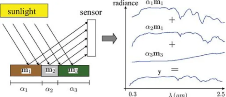
YPERSPECTRAL cameras [1]–[11] contribute signifi-cantly to earth observation and remote sensing [12], [13]. Their potential motivates the development of small, commer-cial, high spatial and spectral resolution instruments. They have also been used in food safety [14]–[17], pharmaceutical process monitoring and quality control [18]–[22], and biomedical, in-dustrial, and biometric, and forensic applications [23]–[27].HSCs can be built to function in many regions of the electro-magnetic spectrum. The focus here is on those covering the vis-ible, near-infrared, and shortwave infrared spectral bands (in the range 0.3 to 2.5 [5]). Disregarding atmospheric effects, the signal recorded by an HSC at a pixel is a mixture of light scattered by substances located in the field of view [3]. Fig. 1 illustrates the measured data. They are organized into planes forming a data cube. Each plane corresponds to radiance ac-quired over a spectral band for all pixels. Each spectral vector corresponds to the radiance acquired at a given location for all spectral bands.
A. Linear and Nonlinear Mixing Models
Hyperspectral unmixing (HU) refers to any process that sep-arates the pixel spectra from a hyperspectral image into a
col-lection of constituent spectra, or spectral signatures, called
end-members and a set of fractional abundances, one set per pixel.
The endmembers are generally assumed to represent the pure materials present in the image and the set of abundances, or simply abundances, at each pixel to represent the percentage of each endmember that is present in the pixel.
There are a number of subtleties in this definition. First, the notion of a pure material can be subjective and problem de-pendent. For example, suppose a hyperspectral image contains spectra measured from bricks laid on the ground, the mortar between the bricks, and two types of plants that are growing through cracks in the brick. One may suppose then that there are four endmembers. However, if the percentage of area that is covered by the mortar is very small then we may not want to have an endmember for mortar. We may just want an end-member for “brick”. It depends on if we have a need to directly measure the proportion of mortar present. If we have need to measure the mortar, then we may not care to distinguish be-tween the plants since they may have similar signatures. On the other hand, suppose that one type of plant is desirable and the other is an invasive plant that needs to be removed. Then we may want two plant endmembers. Furthermore, one may only be interested in the chlorophyll present in the entire scene. Ob-viously, this discussion can be continued ad nauseum but it is clear that the definition of the endmembers can depend upon the application.
The second subtlety is with the proportions. Most researchers assume that a proportion represents the percentage of material associated with an endmember present in the part of the scene imaged by a particular pixel. Indeed, Hapke [28] states that the abundances in a linear mixture represent the relative area of the corresponding endmember in an imaged region. Lab experi-ments conducted by some of the authors have confirmed this in a laboratory setting. However, in the nonlinear case, the situation is not as straightforward. For example, calibration objects can sometimes be used to map hyperspectral measurements to re-flectance, or at least to relative reflectance. Therefore, the coor-dinates of the endmembers are approximations to the reflectance of the material, which we may assume for the sake of argu-ment to be accurate. The reflectance is usually not a linear func-tion of the mass of the material nor is it a linear funcfunc-tion of the cross-sectional area of the material. A highly reflective, yet small object may dominate a much larger but dark object at a pixel, which may lead to inaccurate estimates of the amount of material present in the region imaged by a pixel, but accurate estimates of the contribution of each material to the reflectivity measured at the pixel. Regardless of these subtleties, the large number of applications of hyperspectral research in the past ten years indicates that current models have value.
Unmixing algorithms currently rely on the expected type of mixing. Mixing models can be characterized as either linear or nonlinear [1], [29]. Linear mixing holds when the mixing scale is macroscopic [30] and the incident light interacts with just one material, as is the case in checkerboard type scenes [31], [32]. In this case, the mixing occurs within the instrument itself. It is due to the fact that the resolution of the instrument is not fine enough. The light from the materials, although almost completely sepa-rated, is mixed within the measuring instrument. Fig. 2 depicts
Fig. 2. Linear mixing. The measured radiance at a pixel is a weighted average of the radiances of the materials present at the pixel.
linear mixing: Light scattered by three materials in a scene is incident on a detector that measures radiance in bands. The measured spectrum is a weighted average of the mate-rial spectra. The relative amount of each matemate-rial is represented by the associated weight.
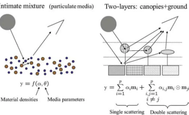
Conversely, nonlinear mixing is usually due to physical inter-actions between the light scattered by multiple materials in the scene. These interactions can be at a classical, or multilayered, level or at a microscopic, or intimate, level. Mixing at the clas-sical level occurs when light is scattered from one or more ob-jects, is reflected off additional obob-jects, and eventually is mea-sured by hyperspectral imager. A nice illustrative derivation of a multilayer model is given by Borel and Gerstl [33] who show that the model results in an infinite sequence of powers of prod-ucts of reflectances. Generally, however, the first order terms are sufficient and this leads to the bilinear model. Microscopic mixing occurs when two materials are homogeneously mixed [28]. In this case, the interactions consist of photons emitted from molecules of one material are absorbed by molecules of another material, which may in turn emit more photons. The mixing is modeled by Hapke as occurring at the albedo level and not at the reflectance level. The apparent albedo of the mixture is a linear average of the albedos of the individual substances but the reflectance is a nonlinear function of albedo, thus leading to a different type of nonlinear model.
Fig. 3 illustrates two non-linear mixing scenarios: the left-hand panel represents an intimate mixture, meaning that the ma-terials are in close proximity; the right-hand panel illustrates a multilayered scene, where there are multiple interactions among the scatterers at the different layers.
Most of this overview is devoted to the linear mixing model. The reason is that, despite its simplicity, it is an acceptable approximation of the light scattering mechanisms in many real scenarios. Furthermore, in contrast to nonlinear mixing, the linear mixing model is the basis of a plethora of unmixing models and algorithms spanning back at least 25 years. A sam-pling can be found in [1], [34]–[47]). Others will be discussed throughout the rest of this paper.
B. Brief Overview of Nonlinear Approaches
Radiative transfer theory (RTT) [48] is a well established mathematical model for the transfer of energy as photons interacts with the materials in the scene. A complete physics based approach to nonlinear unmixing would require inferring
Fig. 3. Two nonlinear mixing scenarios. Left hand: intimate mixture; Right hand: multilayered scene.
the spectral signatures and material densities based on the RTT. Unfortunately, this is an extremely complex ill-posed problem, relying on scene parameters very hard or impossible to obtain. The Hapke [31], Kulbelka-Munk [49] and Shkuratov [50] scattering formulations are three approximations for the analytical solution to the RTT. The former has been widely used to study diffuse reflection spectra in chemistry [51] whereas the later two have been used, for example, in mineral unmixing applications [1], [52].
One wide class of strategies is aimed at avoiding the complex physical models using simpler but physics inspired models, such kernel methods. In [53] and following works [54]–[57], Broad-water et al. have proposed several kernel-based unmixing al-gorithms to specifically account for intimate mixtures. Some of these kernels are designed to be sufficiently flexible to allow several nonlinearity degrees (using, e.g., radial basis functions or polynomials expansions) while others are physics-inspired kernels [55].
Conversely, bilinear models have been successively proposed in [58]–[62] to handle scattering effects, e.g., occurring in the multilayered scene. These models generalize the standard linear model by introducing additional interaction terms. They mainly differ from each other by the additivity constraints imposed on the mixing coefficients [63].
However, limitations inherent to the unmixing algorithms that explicitly rely on both models are twofold. Firstly, they are not multipurpose in the sense that those developed to process intimate mixtures are inefficient in the multiple interaction scenario (and vice versa). Secondly, they generally require the prior knowledge of the endmember signatures. If such infor-mation is not available, these signatures have to be estimated from the data by using an endmember extraction algorithm.
To achieve flexibility, some have resorted to machine learning strategies such as neural networks [64]–[70], to nonlinearly re-duce dimensionality or learn model parameters in a supervised fashion from a collection of examples (see [35] and references therein). The polynomial post nonlinear mixing model intro-duced in [71] seems also to be sufficiently versatile to cover a wide class of nonlinearities. However, again, these algorithms assumes the prior knowledge or extraction of the endmembers. Mainly due to the difficulty of the issue, very few attempts have been conducted to address the problem of fully
unsuper-vised nonlinear unmixing. One must still concede that a sig-nificant contribution has been carried by Heylen et al. in [72] where a strategy is introduced to extract endmembers that have been nonlinearly mixed. The algorithmic scheme is similar in many respects to the well-known N-FINDR algorithm [73]. The key idea is to maximize the simplex volume computed with geodesic measures on the data manifold. In this work, exact geodesic distances are approximated by shortest-path distances in a nearest-neighbor graph. Even more recently, same authors have shown in [74] that exact geodesic distances can be derived on any data manifold induced by a nonlinear mixing model, such as the generalized bilinear model introduced in [62].
Quite recently, Close and Gader have devised two methods for fully unsupervised nonlinear unmixing in the case of in-timate mixtures [75], [76] based on Hapke’s average albedo model cited above. One method assumes that each pixel is either linearly or nonlinearly mixed. The other assumes that there can be both nonlinear and linear mixing present in a single pixel. The methods were shown to more accurately estimate physical mixing parameters using measurements made by Mustard et al. [56], [57], [64], [77] than existing techniques. There is still a great deal of work to be done, including evaluating the useful-ness of combining bilinear models with average albedo models. In summary, although researchers are beginning to expand more aggressively into nonlinear mixing, the research is imma-ture compared with linear mixing. There has been a tremendous effort in the past decade to solve linear unmixing problems and that is what will be discussed in the rest of this paper.
C. Hyperspectral Unmixing Processing Chain
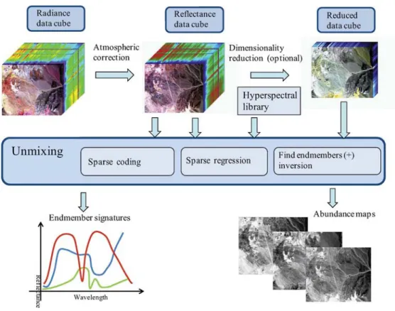
Fig. 4 shows the processing steps usually involved in the hyperspectral unmixing chain: atmospheric correction, di-mensionality reduction, and unmixing, which may be tackled via the classical endmember determination plus inversion, or via sparse regression or sparse coding approaches. Often, endmember determination and inversion are implemented simultaneously. Below, we provide a brief characterization of each of these steps:
1) Atmospheric correction. The atmosphere attenuates and scatterers the light and therefore affects the radiance at the sensor. The atmospheric correction compensates for these effects by converting radiance into reflectance, which is an intrinsic property of the materials. We stress, however, that linear unmixing can be carried out directly on radiance data.
2) Data reduction. The dimensionality of the space spanned by spectra from an image is generally much lower than available number of bands. Identifying appropriate sub-spaces facilitates dimensionality reduction, improving algorithm performance and complexity and data storage. Furthermore, if the linear mixture model is accurate, the signal subspace dimension is one less than equal to the number of endmembers, a crucial figure in hyperspectral unmixing.
3) Unmixing. The unmixing step consists of identifying the endmembers in the scene and the fractional abundances at each pixel. Three general approaches will be discussed here. Geometrical approaches exploit the fact that linearly
Fig. 4. Schematic diagram of the hyperspectral unmixing process.
Fig. 5. Illustration of the simplex set for ( is the convex hull of the columns of , ). Green circles represent spectral vectors. Red circles represent vertices of the simplex and correspond to the endmembers.
mixed vectors are in a simplex set or in a positive cone.
Statistical approaches focus on using parameter
estima-tion techniques to determine endmember and abundance parameters. Sparse regression approaches, which formu-lates unmixing as a linear sparse regression problem, in a fashion similar to that of compressive sensing [78], [79]. This framework relies on the existence of spectral libraries usually acquired in laboratory. A step forward, termed
sparse coding [80], consists of learning the dictionary
from the data and, thus, avoiding not only the need of libraries but also calibration issues related to different conditions under which the libraries and the data were acquired.
4) Inversion. Given the observed spectral vectors and the identified endmembers, the inversion step consists of
solving a constrained optimization problem which mini-mizes the residual between the observed spectral vectors and the linear space spanned by the inferred spectral signatures; the implicit fractional abundances are, very often, constrained to be nonnegative and to sum to one (i.e., they belong to the probability simplex). There are, however, many hyperspectral unmixing approaches in which the endmember determination and inversion steps are implemented simultaneously.
The remainder of the paper is organized as follows. Section II describes the linear spectral mixture model adopted as the base-line model in this contribution. Section III describes techniques for subspace identification. Sections IV, , , VII describe four classes of techniques for endmember and fractional abundances estimation under the linear spectral unmixing. Sections IV and V are devoted to the longstanding geometrical and statistical based approaches, respectively. Sections VI and VII are devoted to the recently introduced sparse regression based unmixing and to the exploitation of the spatial contextual information, respec-tively. Each of these sections introduce the underlying mathe-matical problem and summarizes state-of-the-art algorithms to address such problem.
Experimental results obtained from simulated and real data sets illustrating the potential and limitations of each class of al-gorithms are described. The experiments do not constitute an exhaustive comparison. Both code and data for all the exper-iments described here are available at http://www.lx.it.pt/~bi-oucas/code/unmixing_overview.zip. The paper concludes with a summary and discussion of plausible future developments in the area of spectral unmixing.
Fig. 6. Illustration of the concept of simplex of minimum volume containing the data for three data sets. The endmembers in the left hand side and in the middle are identifiable by fitting a simplex of minimum volume to the data, whereas this is not applicable to the right hand side data set. The former data set correspond to a highly mixed scenario.
II. LINEARMIXTUREMODEL
If the multiple scattering among distinct endmembers is neg-ligible and the surface is partitioned according to the fractional abundances, as illustrated in Fig. 2, then the spectrum of each pixel is well approximated by a linear mixture of endmember spectra weighted by the corresponding fractional abundances [1], [3], [29], [39]. In this case, the spectral measurement1 at
channel ( is the total number of channels) from a given pixel, denoted by , is given by the linear mixing
model (LMM)
(1)
where denotes the spectral measurement of endmember at the spectral band, denotes the frac-tional abundance of endmember , denotes an additive per-turbation (e.g., noise and modeling errors), and denotes the number of endmembers. At a given pixel, the fractional abun-dance , as the name suggests, represents the fractional area occupied by the th endmember. Therefore, the fractional abun-dances are subject to the following constraints:
(2)
i.e., the fractional abundance vector
(the notation indicates vector transposed) is in the standard -simplex (or unit -simplex). In HU jargon, the nonnegativity and the sum-to-one constraints are termed
abun-dance nonnegativity constraint (ANC) and abunabun-dance sum con-straint (ASC), respectively. Researchers may sometimes expect
that the abundance fractions sum to less than one since an algo-rithm may not be able to account for every material in a pixel; it is not clear whether it is better to relax the constraint or to simply consider that part of the modeling error.
Let denote a -dimensional column vector, and denote the spectral signature of the th endmember. Expression (1) can then be written as
(3)
1Although the type of spectral quantity (radiance, reflectance, etc.) is
impor-tant when processing data, specification is not necessary to derive the mathe-matical approaches.
where is the mixing matrix containing the signatures of the endmembers present in the covered area, and . Assuming that the columns of are affinely independent, i.e.,
are linearly independent, then the set
i.e., the convex hull of the columns of , is a -simplex in . Fig. 5 illustrates a 2-simplex for a hypothetical mixing matrix containing three endmembers. The points in green de-note spectral vectors, whereas the points in red are vertices of the simplex and correspond to the endmembers. Note that the inference of the mixing matrix is equivalent to identifying the vertices of the simplex . This geometrical point of view, exploited by many unmixing algorithms, will be further devel-oped in Section IV-B.
Since many algorithms adopt either a geometrical or a sta-tistical framework [34], [36], they are a focus of this paper. To motivate these two directions, let us consider the three data sets shown in Fig. 6 generated under the linear model given in (3) where the noise is assumed to be negligible. The spectral vec-tors generated according to (3) are in a simplex whose vertices correspond to the endmembers. The left hand side data set con-tains pure pixels, i.e, for any of the endmembers there is at least one pixel containing only the correspondent material; the data set in the middle does not contain pure pixels but contains at least spectral vectors on each facet. In both data sets (left and middle), the endmembers may by inferred by fitting a minimum volume (MV) simplex to the data; this rather simple and yet powerful idea, introduced by Craig in his seminal work [81], underlies several geometrical based unmixing algorithms. A similar idea was introduced in 1989 by Perczel in the area of Chemometrics et al. [82].
The MV simplex shown in the right hand side example of Fig. 6 is smaller than the true one. This situation corresponds to a highly mixed data set where there are no spectral vectors near the facets. For these classes of problems, we usually re-sort to the statistical framework in which the estimation of the mixing matrix and of the fractional abundances are formulated as a statistical inference problem by adopting suitable proba-bility models for the variables and parameters involved, namely for the fractional abundances and for the mixing matrix.
Fig. 7. Illustration of a badly-conditioned mixing matrices and noise (repre-sented by uncertainty regions) centered on clean spectral vectors repre(repre-sented by green circles.
Fig. 8. Signal-to-noise-ratio spectral distribution (SNR-SD) for the data sets SudP5SNR40, SusgsP5SNR40, and Rcuprite. The first two are simulated and contain endmembers and the third is a subset of the AVIRIS Cuprite data set.
A. Characterization of the Spectral Unmixing Inverse Problem
Given the data set containing -dimensional spectral vectors, the linear HU problem is, with reference to the linear model (3), the estimation of the mixing matrix and of the fractional abundances vectors corre-sponding to pixels . This is often a difficult inverse problem, because the spectral signatures tend to be strongly cor-related, yielding badly-conditioned mixing matrices and, thus, HU estimates can be highly sensitive to noise. This scenario is illustrated in Fig. 7, where endmembers and are very close, thus yielding a badly-conditioned matrix , and the ef-fect of noise is represented by uncertainty regions.
To characterize the linear HU inverse problem, we use the
signal-to-noise-ratio (SNR)
where and are, respectively, the signal (i.e., ) and noise correlation matrices and denotes expected value. Besides SNR, we introduce the signal-to-noise-ratio spectral
distribution (SNR-SD) defined as
(4)
where is the eigenvalue-eigenvector couple of ordered by decreasing value of . The ratio
yields the signal-to-noise ratio (SNR) along the signal direc-tion . Therefore, we must have for , in order to obtain acceptable unmixing results.
Otherwise, there are directions in the signal subspace signifi-cantly corrupted by noise.
Fig. 8 plots , in the interval , for the following data sets:
• SudP5SNR40: simulated; mixing matrix sampled from a uniformly distributed random variable in the in-terval [0, 1]; ; ; fractional abundances dis-tributed uniformly on the 4-unit simplex; . • SusgsP5SNR40: simulated; mixing matrix sampled
from the United States Geological Survey (USGS) spec-tral library;2 ; ; fractional abundances
dis-tributed uniformly on the 4-unit simplex; . • Rcuprite: real; subset of the well-known AVIRIS cuprite
data cube3 with size 250 lines by 191 columns by 188
bands (noisy bands were removed).
The signal and noise correlation matrices were obtained with the algorithms and code distributed with HySime [83]. From those plots, we read that, for SudP5SNR40 data set,
for and for , indicating that the SNR is high in the signal subspace. For SusgsP5SNR40, the singular values of the mixing matrix decay faster due to the high correlation of the USGS spectral signatures. Neverthe-less the “big picture” is similar to that of SudP5SNR40 data set. The Rcuprite data set yields the more difficult inverse problem because has “close to convex shape” slowly ap-proaching the value 1. This is a clear indication of a badly-con-ditioned inverse problem [84].
III. SIGNALSUBSPACEIDENTIFICATION
The number of endmembers present in a given scene is, very often, much smaller than the number of bands . Therefore, as-suming that the linear model is a good approximation, spectral vectors lie in or very close to a low-dimensional linear subspace. The identification of this subspace enables low-dimensional yet accurate representation of spectral vectors, thus yielding gains in computational time and complexity, data storage, and SNR. It is usually advantageous and sometimes necessary to operate on data represented in the signal subspace. Therefore, a signal sub-space identification algorithm is required as a first processing step.
Unsupervised subspace identification has been approached in many ways. Band selection or band extraction, as the name sug-gests, exploits the high correlation existing between adjacent bands to select a few spectral components among those with higher SNR [85], [86]. Projection techniques seek for the best subspaces to represent data by optimizing objective functions. For example, principal component analysis (PCA) [87] mini-mizes sums of squares; singular value decomposition (SVD) [88] maximizes power; projections on the first eigenvectors of the empirical correlation matrix maximize likelihood, if the noise is additive and white and the subspace dimension is known to be [88]; maximum noise fraction (MNF) [89] and noise
ad-justed principal components (NAPC) [90] minimize the ratio of
noise power to signal power. NAPC is mathematically equiva-lent to MNF [90] and can be interpreted as a sequence of two
2http://speclab.cr.usgs.gov/spectral-lib.html 3http://aviris.jpl.nasa.gov/data/free\_data.html
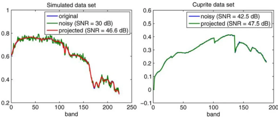
Fig. 9. Left: Noisy and projected spectra from the simulates data set SusgsP5SNR30. Right: Noisy and projected spectra from the real data set Rcuprite
principal component transforms: the first applies to the noise and the second applies to the transformed data set. MNF is re-lated to SNR-SD introduced in (4). In fact, both metrics are equivalent in the case of white noise, i.e, , where de-notes the identity matrix. However, they differ when . The optical real-time adaptive spectral identification system (ORASIS) [91] framework, developed by U. S. Naval Research Laboratory aiming at real-time data processing, has been used both for dimensionality reduction and endmember extraction. This framework consists of several modules, where the dimen-sion reduction is achieved by identifying a subset of exemplar pixels that convey the variability in a scene. Each new pixel collected from the scene is compared to each exemplar pixel by using an angle metric. The new pixel is added to the exemplar set if it is sufficiently different from each of the existing exemplars. An orthogonal basis is periodically created from the current set of exemplars using a modified Gram-Schmidt procedure [92].
The identification of the signal subspace is a model order inference problem to which information theoretic criteria like the minimum description length (MDL) [93], [94] or the
Akaike information criterion (AIC) [95] comes to mind. These
criteria have in fact been used in hyperspectral applications [96] adopting the approach introduced by Wax and Kailath in [97]. In turn, Harsanyi, Farrand, and Chang [98] developed a Neyman-Pearson detection theory-based thresholding method (HFC) to determine the number of spectral endmembers in hyperspectral data, referred to in [96] as virtual dimensionality (VD). The HFC method is based on a detector built on the eigenvalues of the sample correlation and covariance matrices. A modified version, termed noise-whitened HFC (NWHFC), includes a noise-whitening step [96]. HySime ( hyperspectral
signal identification by minimum error) [83] adopts a minimum
mean squared error based approach to infer the signal subspace. The method is eigendecomposition based, unsupervised, and fully-automatic (i.e., it does not depend on any tuning parame-ters). It first estimates the signal and noise correlation matrices and then selects the subset of eigenvalues that best represents the signal subspace in the least square error sense.
When the spectral mixing is nonlinear, the low dimensional subspace of the linear case is often replaced with a low di-mensional manifold, a concept defined in the mathematical
subject of topology [99]. A variety of local methods exist for estimating manifolds. For example, curvilinear component analysis [100], curvilinear distance analysis [101], manifold learning [102]–[107] are non-linear projections based on the preservation of the local topology. Independent component analysis [108], [109], projection pursuit [110], [111], and wavelet decomposition [112], [113] have also been considered.
A. Projection on the Signal Subspace
Assume that the signal subspace, denoted by , has been identified by using one of the above referred to methods and let the columns of be an orthonormal basis for , where , for . The coordinates of the orthogonal projection of a spectral vector onto , with respect to the basis , are given by . Replacing
by the observation model (3), we have
As referred to before, projecting onto a signal subspace can yield large computational, storage, and SNR gains. The first two are a direct consequence of the fact that in most applica-tions; to briefly explain the latter, let us assume that the noise is zero-mean and has covariance . The mean power of the projected noise term is then ( de-notes mean value). The relative attenuation of the noise power implied by the projection is then .
Fig. 9 illustrates the advantages of projecting the data sets on the signal subspace. The noise and the signal subspace were es-timated with HySime [83]. The plot on the left hand side shows a noisy and the corresponding projected spectra taken from the simulated data set SusgsP5SNR30.4 The subspace dimension
was correctly identified. The SNR of the projected data set is 46.6 dB, which is above to that of the noisy data set. The plot on the right hand side shows a noisy and the corresponding projected spectra from the Rcuprite data set. The identified subspace dimension has dimension 18. The SNR of the projected data set is 47.5 dB, which is 5 dB above to that
4Parameters of the simulated data set SusgsP5SNR30: mixing matrix
sampled from a uniformly distributed random variable in the interval [0, 1]; ; ; fractional abundances distributed uniformly on the 4-unit simplex; .
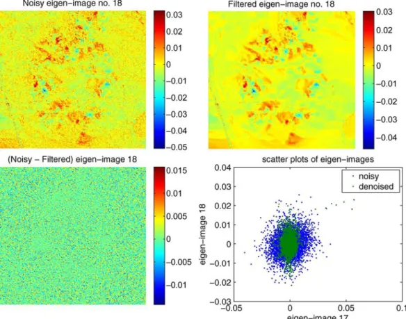
Fig. 10. Top left: noisy eigen-image no. 18 of the Rcuprite data set. Top right: denoised no. 18; Bottom left: difference between noisy and denoised images. Botton right: scatter plots of the Eigen-image no. 17 and no. 18 of the Rcuprite data set (blue dots: noisy data; Green dots: denoised data).
Fig. 11. Projections of the observed data onto an hyperplane: (a) Orthogonal projection on an hyperplane (the projected vectors suffers a rotation); (b) Per-spective projection (the scaling brings them to the hyperplane defined by ).
of the noisy data set. The colored nature of the additive noise explains the difference .
A final word of warning: although the projection of the data set onto the signal subspace often removes a large percentage of the noise, it does not improve the conditioning of the HU inverse problem, as this projection does not change the values of for the signal subspace eigen-components.
A possible line of attack to further reduce the noise in the signal subspace is to exploit spectral and spatial contextual in-formation. We give a brief illustration in the spatial domain. Fig. 10, on the top left hand side, shows the eigen-image no. 18, i.e., the image obtained from for , of the Rcuprite data set. The basis of the signal subspace were obtained with the HySime algorithm. A filtered version using then BM3D [114]
is shown on the top right hand side. The denoising algorithm is quite effective in this example, as confirmed by the absence of structure in the noise estimate (the difference between the noisy and the denoised images) shown in the bottom left hand side image. This effectiveness can also be perceived from the scatter plots of the noisy (blue dots) and denoised (green dots) eigen-images 17 and 18 shown in the bottom right hand side figure. The scatter plot corresponding to the denoised image is much more dense, reflecting the lower variance.
B. Affine Set Projection
From now on, we assume that the observed data set has been projected onto the signal subspace and, for simplicity of nota-tion, we still represent the projected vectors as in (3), that is,
(5) where and . Since the columns of be-long to the signal subspace, the original mixing matrix is simply given by the matrix product .
Model (5) is a simplification of reality, as it does not model pixel-to-pixel signature variability. Signature variability has been studied and accounted for in a few unmixing algorithms (see, e.g., [115]–[118]), including all statistical algorithms that treat endmembers as distributions. Some of this variability is amplitude-based and therefore primarily characterized by spectral shape invariance [38]; i.e., while the spectral shapes of the endmembers are fairly consistent, their amplitudes are variable. This implies that the endmember signatures are af-fected by a positive scale factor that varies from pixel to pixel.
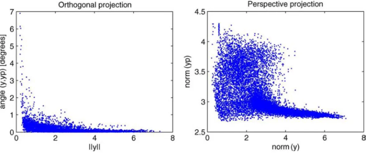
Fig. 12. Left (orthogonal projection): angles between projected and unprojected vectors. Right (perspective projection): scale factors between projected and un-projected vectors.
Hence, instead of one matrix of endmember spectra for the entire scene, there is a matrix of endmember spectra for each
pixel for . In
this case, and in the absence of noise, the observed spectral vectors are no longer in a simplex defined by a fixed set of endmembers but rather in the set
(6)
as illustrated in Fig. 11. Therefore, the coefficients of the end-member spectra need not sum-to-one, although they are still nonnegative. Transformations of the data are required to im-prove the match of the model to reality. If a true mapping from units of radiance to reflectance can be found, then that transfor-mation is sufficient. However, estimating that mapping can be difficult problem or impossible. Other methods can be applied to to ensure that the sum-to-one constraint is a better model, such as the following:
a) Orthogonal projection: Use PCA to identify the affine set that best represent the observed data in the least squares sense and then compute the orthogonal projec-tion of the observed vectors onto this set (see [119] for details). This projection is illustrated in Fig. 11.
b) Perspective projection: This is the so-called dark point fixed transform (DPFT) proposed in [81]. For a given observed vector , this projection, illustrated in Fig. 11, amounts to rescale according to , where is chosen such that for every in the data set. The hyperplane containing the projected vectors is defined by
, for any .
Notice that the orthogonal projection modifies the direction of the spectral vectors whereas the perspective projection does not. On the other hand, the perspective projection introduces large scale factors, which may become negative, for spectral vectors close to being orthogonal to . Furthermore, vectors with different angles produce non-parallel affine sets and thus different fractional abundances, which implies that the choice of is a critical issue for accurate estimation.
These effects are illustrated in Fig. 12 for the Rterrain data set.5 This is a publicly available hyperspectral data cube
distributed by the Army Geospatial Center, United States Army Corps of Engineers, and was collected by the hyperspectral image data collection experiment (HYDICE). Its dimensions are 307 pixels by 500 lines and 210 spectral bands. The figure on the left hand side plots the angles between the unprojected and the orthogonally projected vectors, as a function of the norm of the unprojected vectors. The higher angles, of the order of 1–7 , occur for vectors of small norm, which usually correspond to shadowed areas. The figure on the right hand side plots the norm of the projected vectors as a function of the norm of the unprojected vectors. The corresponding scale factors varies between, approximately, between 1/3 and 10.
A possible way of mitigating these projection errors is dis-carding the problematic projections, which are vectors with an-gles between projected and unprojected vectors larger than a given small threshold, in the case of the perspective projection, and vectors with very small or negative scale factors , in the case of the orthogonal projection.
IV. GEOMETRICALBASED APPROACHES TOLINEAR
SPECTRALUNMIXING
The geometrical-based approaches are categorized into two main categories: Pure Pixel (PP) based and Minimum Volume (MV) based. There are a few other approaches that will also be discussed.
A. Geometrical Based Approaches: Pure Pixel Based Algorithms
The pure pixel based algorithms still belong to the MV class but assume the presence in the data of at least one pure pixel per endmember, meaning that there is at least one spectral vector on each vertex of the data simplex. This assumption, though enabling the design of very efficient algorithms from the com-putational point of view, is a strong requisite that may not hold in many datasets. In any case, these algorithms find the set of most pure pixels in the data. They have probably been the most
often used in linear hyperspectral unmixing applications, per-haps because of their light computational burden and clear con-ceptual meaning. Representative algorithms of this class are the following:
• The pixel purity index (PPI) algorithm [120], [121] uses MNF as a preprocessing step to reduce dimensionality and to improve the SNR. PPI projects every spectral vector onto skewers, defined as a large set of random vectors. The points corresponding to extremes, for each skewer direc-tion, are stored. A cumulative account records the number of times each pixel (i.e., a given spectral vector) is found to be an extreme. The pixels with the highest scores are the purest ones.
• N-FINDR [73] is based on the fact that in spectral di-mensions, the volume defined by a simplex formed by the purest pixels is larger than any other volume defined by any other combination of pixels. This algorithm finds the set of pixels defining the largest volume by inflating a sim-plex inside the data.
• The iterative error analysis (IEA) algorithm [122] imple-ments a series of linear constrained unmixings, each time choosing as endmembers those pixels which minimize the remaining error in the unmixed image.
• The vertex component analysis (VCA) algorithm [123] it-eratively projects data onto a direction orthogonal to the subspace spanned by the endmembers already determined. The new endmember signature corresponds to the extreme of the projection. The algorithm iterates until all endmem-bers are exhausted.
• The simplex growing algorithm (SGA) [124] iteratively grows a simplex by finding the vertices corresponding to the maximum volume.
• The sequential maximum angle convex cone (SMACC) al-gorithm [125] is based on a convex cone for representing the spectral vectors. The algorithm starts with a single end-member and increases incrementally in dimension. A new endmember is identified based on the angle it makes with the existing cone. The data vector making the maximum angle with the existing cone is chosen as the next end-member to enlarge the endend-member set. The algorithm ter-minates when all of the data vectors are within the convex cone, to some tolerance.
• The alternating volume maximization (AVMAX) [126], in-spired by N-FINDR, maximizes, in a cyclic fashion, the volume of the simplex defined by the endmembers with respect to only one endmember at one time. AVMAX is quite similar to the SC-N-FINDR variation of N-FINDR introduced in [127].
• The successive volume maximization (SVMAX) [126] is similar to VCA. The main difference concerns the way data is projected onto a direction orthogonal the subspace spanned by the endmembers already determined. VCA considers a random direction in these subspace, whereas SVMAX considers the complete subspace.
• The collaborative convex framework [128] factorizes the data matrix into a nonnegative mixing matrix and a sparse and also nonnegative abundance matrix . The
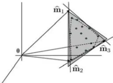
Fig. 13. Illustration of the concept of simplex of minimum volume containing the data.
columns of the mixing matrix are constrained to be columns of the data .
• Lattice Associative Memories (LAM) [129]–[131] model
sets of spectra as elements of the lattice of partially or-dered real-valued vectors. Lattice operations are used to nonlinearly construct LAMS. Endmembers are found by constructing so-called min and max LAMs from spectral pixels. These LAMs contain maximum and minimum coordinates of spectral pixels (after appropriate additive scaling) and are candidate endmembers. Endmembers are selected from the LAMS using the notions of affine inde-pendence and similarity measures such as spectral angle, correlation, mutual information, or Chebyschev distance. Algorithms AVMAX and SVMAX were derived in [126] under a continuous optimization framework inspired by Winter’s maximum volume criterium [73], which underlies N-FINDR. Following a rigorous approach, Chan et al. not only derived AVMAX and SVMAX, but have also unveiled a number of links between apparently disparate algorithms such as N-FINDR and VCA.
B. Geometrical Based Approaches: Minimum Volume Based Algorithms
The MV approaches seek a mixing matrix that minimizes the volume of the simplex defined by its columns, referred to as , subject to the constraint that contains the observed spectral vectors. The constraint can be soft or hard. The pure pixel constraint is no longer enforced, resulting in a much harder nonconvex optimization problem. Fig. 13 further illustrates the concept of simplex of minimum size containing the data. The estimated mixing matrix dif-fers slightly from the true mixing matrix because there are not enough data points per facet (necessarily per facet) to de-fine the true simplex.
Let us assume that the data set has been projected onto the signal subspace , of dimension , and that the vectors
, for , are affinely independent (i.e., , for , are linearly independent). The dimensionality of the simplex is therefore so the volume of is zero in . To obtain a nonzero volume, the ex-tended simplex , containing the origin, is usually considered. We recall that the volume of , the convex hull of , is given by
Fig. 14. Noisy data. The dashed simplex represents the simplex of minimum volume required to contain all the data; by allowing violations to the positivity constraint, the MVSA and SISAL algorithms yield a simplex very close to the true one.
An alternative to (7) consists of shifting the data set to the origin and working in the subspace of dimension . In this case, the volume of the simplex is given by
Craig’s work [81], published in 1994, put forward the seminal concepts regarding the algorithms of MV type. After identifying the subspace and applying projective projection (DPFT), the al-gorithm iteratively changes one facet of the simplex at a time, holding the others fixed, such that the volume
is minimized and all spectral vectors belong to this simplex; i.e., and (respectively, ANC and ASC constraints6) for . In a more formal way:
The minimum volume simplex analysis (MVSA) [132] and the simplex identification via variable splitting and augmented Lagrangian (SISAL) [133] algorithms implement a robust ver-sion of the MV concept. The robustness is introduced by al-lowing the positivity constraint to be violated. To grasp the rel-evance of this modification, noisy spectral vectors are depicted in Fig. 14. Due to the presence of noise, or any other pertur-bation source, the spectral vectors may lie outside the true data simplex. The application of a MV algorithm would lead to the dashed estimate, which is far from the original.
In order to estimate endmembers more accurately, MVSA/ SISAL allows violations to the positivity constraint. Violations are penalized using the hinge function ( if
6The notation stands for a column vector of ones with size .
and if ). MVSA/SISAL project the data onto a signal subspace. Thus the representation of Section III-B is used. Con-sequently, the matrix is square and theoretically invertible (ill-conditioning can make it difficult to compute the inverse nu-merically). Furthermore,
(8) MVSA/SISAL aims at solving the following optimization problem:
(9)
(10)
where with being any set of
of linearly independent spectral vectors taken from the data set is a regularization parameter, and stands for the number of spectral vectors.
We make the following two remarks: a) maximizing is equivalent to minimizing ; b) the term weights the ANC violations. As approaches infinity, the soft constraint approaches the hard constraint. MVSA/SISAL optimizes by solving a sequence of convex optimization problems using the method of augmented Lagrange multipliers, resulting in a computationally efficient algorithm.
The minimum volume enclosing simplex (MVES) [134] aims at solving the optimization problem (10) with , i.e., for hard positivity constraints. MVES implements a cyclic mini-mization using linear programs (LPs). Although the optimiza-tion problem (10) is nonconvex, it is proved in (10) that the existence of pure pixels is a sufficient condition for MVES to identify the true endmembers.
A robust version of MVES (RMVES) was recently intro-duced in [135]. RMVES accounts for the noise effects in the observations by employing chance constraints, which act as soft constraints on the fractional abundances. The chance con-straints control the volume of the resulting simplex. Under the Gaussian noise assumption, RMVES infers the mixing matrix and the fractional abundances via alternating optimization involving quadratic programming solvers.
The minimum volume transform-nonnegative matrix factor-ization (MVC-NMF) [136] solves the following optimfactor-ization problem applied to the original data set, i.e., without dimension-ality reduction:
(11) where is a matrix containing the frac-tional abundances is the Frobenius norm of matrix and is a regularization parameter. The optimiza-tion (11) minimizes a two term objective funcoptimiza-tion, where the
term measures the approximation error and the term measures the square of the volume of the sim-plex defined by the columns of . The regularization param-eter controls the tradeoff between the reconstruction errors and simplex volumes. MVC-NMF implements a sequence of alternate minimizations with respect to (quadratic program-ming problem) and with respect to (nonconvex program-ming problem). The major difference between MVC-NMF and MVSA/SISAL/RMVES algorithms is that the latter allows vio-lations of the ANC, thus bringing robustness to the SU inverse problem, whereas the former does not.
The iterative constrained endmembers (ICE) algorithm [137] aims at solving an optimization problem similar to that of MVC-NMF, where the volume of the simplex is replaced by a much more manageable approximation: the sum of squared distances between all the simplex vertices. This volume regu-larizer is quadratic and well defined in any ambient dimension and in degenerated simplexes. These are relevant advantages over the regularizer, which is non-convex and prone to complications when the HU problem is badly conditioned or if the number of endmembers is not exactly known. Variations of these ideas have recently been proposed in [138]–[141]. ICE implements a sequence of alternate minimizations with respect to and with respect to . An advantage of ICE over MVC-NMF, resulting from the use of a quadratic volume regularizer, is that in the former one minimization is a quadratic programming problem while the other is a least squares problem that can be solved analytically, whereas in the MVC-NMF the optimization with respect to is a nonconvex problem. The sparsity-promoting ICE (SPICE) [142] is an extension of the ICE algorithm that incorporates sparsity-promoting priors aiming at finding the correct number of endmembers. Linear terms are added to the quadratic objective function, one for all the proportions associated with one endmember. The linear term corresponds to an exponential prior. A large number of endmembers are used in the initialization. The prior tends to push all the proportions associated with particular endmembers to zero. If all the proportions corresponding to an endmember go to zero, then that endmember can be discarded. The addi-tion of the sparsity promoting prior does not incur addiaddi-tional complexity to the model as the minimization still involves a quadratic program.
The quadratic volume regularizer used in the ICE and SPICE algorithms also provides robustness in the sense of allowing data points to be outside of the simplex . It has been shown that the ICE objective function can be written in the fol-lowing way:
(12)
where is the sample covariance matrix of the endmembers and is a regularization parameter that controls the tradeoff between error and smaller simplexes. If , then the best solution is to shrink all the endmembers to a single point, so all the data will be outside of the simplex. If , then the
best solution is one that yields no error, regardless of the size of the simplex. The solution can be sensitive to the choice of . The SPICE algorithm has the same properties. versions also exist [143].
It is worth noting the both Heylen et al. [144] and Silvn-Cr-denas [145] have reported geometric-based methods that can either search for or analytically solve for the fully constrained least squares solution.
The -NMF method introduced in [146] formulates a non-negative matrix factorization problem similar to (11), where the volume regularizer is replaced with the sparsity-enforcing reg-ularizer . By promoting zero or small abundance fractions, this regularizer pulls endmember facets towards the data cloud having an effect similar to the volume regularizer. The estimates of the endmembers and of the fractional abundances are obtained by a modification of the multiplicative update rules introduced in [147].
Convex cone analysis (CCA) [148], finds the boundary points of the data convex cone (it does not apply affine projection), what is very close to MV concept. CCA starts by selecting the eigenvectors corresponding to the largest eigenvalues. These eigenvectors are then used as a basis to form linear combina-tions that have only nonnegative elements, thus belonging to a convex cone. The vertices of the convex cone correspond to spectral vectors contains as many zero elements as the number of eigenvectors minus one.
Geometric methods can be extended to piecewise linear mixing models. Imagine the following scenario: An airborne hyperspectral imaging sensor acquires data over an area. Part of the area consists of farmland containing alternating rows of two types of crops (crop A and crop B) separated by soil whereas the other part consists of a village with paved roads, buildings (all with the same types of roofs), and non-deciduous trees. Spectra measured from farmland are almost all linear mixtures of endmember spectra associated with crop A, crop B, and soil. Spectra over the village are almost all linear mixtures of endmember spectra associated with pavement, roofs, and non-deciduous trees. Some pixels from the boundary of the village and farmland may be mixtures of all six endmember spectra. The set of all pixels from the image will then consist of two simplexes. Linear unmixing may find some, perhaps all, of the endmembers. However, the model does not accurately represent the true state of nature. There are two convex regions and the vertices (endmembers) from one of the convex regions may be in the interior of the convex hull of the set of all pixels. In that case, an algorithm designed to find extremal points on or outside the convex hull of the data will not find those endmembers (unless it fails to do what it was designed to do, which can happen). Relying on an algorithm failing to do what it is designed to do is not a desirable strategy. Thus, there is a need to devise methods for identifying multiple simplexes in hyperspectral data. One can refer to this class of algorithms as piecewise convex or piecewise linear unmixing.
One approach to designing such algorithms is to represent the convex regions as clusters. This approach has been taken in [149]–[153]. The latter methods are Bayesian and will therefore be discussed in the next section. The first two rely on algorithms derived from fuzzy and possibilistic clustering. Crisp clustering
Fig. 15. Unmixing results of N-FINDR, VCA, MVC-NMF, and SISAL on different data sets: SusgsP5PPSNR30—pure-pixel (top-left); SusgsP5SNR30—non pure pixel (top right); SusgsP5MP08SNR30—truncated fractional abundances (bottom left); SusgsP5XS10SNR30—and highly mixed (bottom tight).
algorithms (such as k-means) assign every data point to one and only one cluster. Fuzzy clustering algorithms allow every data point to be assigned to every cluster to some degree. Fuzzy clus-ters are defined by these assignments, referred to as member-ship functions. In the example above, there should be two clus-ters. Most points should be assigned to one of the two clusters with high degree. Points on the boundary, however, should be assigned to both clusters.
Assuming that there are simplexes in the data, then the fol-lowing objective function can be used to attempt to find end-member spectra and abundances for each simplex:
(13) such that
Here, represents the membership of the data point in the simplex. The other terms are very similar to those used in the ICE/SPICE algorithms except that there are endmember
matrices and abundance vectors. Analytic update formulas can be derived for the memberships, the endmember updates, and the Lagrange multipliers. An update formula can be used to update the fractional abundances but they are sometimes nega-tive and are then clipped at the boundary of the feasible region. One can still use quadratic programming to solve for them. As is the case for almost all clustering algorithms, there are local minima. However, the algorithm using all update formulas is computationally efficient. A robust version also exists that uses a combination of fuzzy and possibilistic clustering [151].
Fig. 15 shows results of pure pixel based algorithms (N-FINDR and VCA) and MV based algorithms (MVC-NMF and SISAL) in simulated data sets representative of the classes of problems illustrated in Fig. 6. These data sets have
pixels and and the following characteristics: SusgsP5PPSNR30—pure pixels and abundances uniformly distributed over the simplex (top left); SusgsP5SNR30 non pure pixels and abundances uniformly distributed over the sim-plex (top right); SusgsP5MP08SNR30 abundances uniformly distributed over the simplex but truncated to 0.8 (bottom left); SusgsP5XS10SNR30 abundances with Dirichlet distributed with concentration parameter set to 10, thus yielding a highly mixed data set.
In the top left data set all algorithm produced very good re-sults because pure pixels are present. In the top right SISAL
and MVC-NMF produce good results but VCA and N-FINDR shows a degradation in performance because there are no pure pixels. In the bottom left SISAL and MVC-NMF still produce good results but VCA and N-FINDR show a significant degra-dation in performance because the pixels close to the vertices were removed. Finally, in the bottom right all algorithm produce unacceptable results because there are no pixels in the vertex of the simplex neither on its facets. These data sets are beyond the reach of geometrical based algorithms.
V. STATISTICALMETHODS
When the spectral mixtures are highly mixed, the geometrical based methods yields poor results because there are not enough spectral vectors in the simplex facets. In these cases, the statis-tical methods are a powerful alternative, which, usually, comes with price: higher computational complexity, when compared with the geometrical based approaches. Statistical methods also provide a natural framework for representing variability in end-members. Under the statistical framework, spectral unmixing is formulated as a statistical inference problem.
Since, in most cases, the number of substances and their re-flectances are not known, hyperspectral unmixing falls into the class of blind source separation problems [154]. Independent Component Analysis (ICA), a well-known tool in blind source separation, has been proposed as a tool to blindly unmix hyper-spectral data [155]–[157]. Unfortunately, ICA is based on the assumption of mutually independent sources (abundance frac-tions), which is not the case of hyperspectral data, since the sum of abundance fractions is constant, implying statistical depen-dence among them. This dependepen-dence compromises ICA appli-cability to hyperspectral data as shown in [39], [158]. In fact, ICA finds the endmember signatures by multiplying the spectral vectors with an unmixing matrix which minimizes the mutual information among channels. If sources are independent, ICA provides the correct unmixing, since the minimum of the mutual information corresponds to and only to independent sources. This is no longer true for dependent fractional abundances. Nev-ertheless, some endmembers may be approximately unmixed. These aspects are addressed in [158].
Bayesian approaches have the ability to model statistical vari-ability and to impose priors that can constrain solutions to phys-ically meaningful ranges and regularize solutions. The latter property is generally considered to be a requirement for solving ill-posed problems. Adopting a Bayesian framework, the infer-ence engine is the posterior density of the random quantities to be estimated. When the unknown mixing matrix and the abundance fraction matrix are assumed to be a priori indepen-dent, the Bayes paradigm allows the joint posterior of and to be computed as
(14) where the notation and stands for the probability density function (pdf) of and of given , respectively. In (14), is the likelihood function depending on the observation model and the prior distribution
and summarize the prior knowledge regarding these unknown parameters.
A popular Bayesian estimator is [159] the joint maximum a
posteriori (MAP) estimator given by
(15)
(16) Under the linear mixing model and assuming the noise random vector is Gaussian with covariance matrix , then, we have . It is then clear that ICE/SPICE [142] and MVC-NMF [136] algo-rithms, which have been classified as geometrical, can also be classified as statistical, yielding joint MAP estimates in (15). In all these algorithms, the estimates are obtained by minimizing a two-term objective function: plays the role of a data fitting criterion and
consists of a penalization. Conversely, from a Bayesian perspec-tive, assigning prior distributions and to the end-member and abundance matrices and , respectively, is a convenient way to ensure physical constraints inherent to the observation model.
The work [160] introduces a Bayesian approach where the linear mixing model with zero-mean white Gaussian noise of covariance is assumed, the fractional abundances are uni-formly distributed on the simplex, and the prior on is an au-toregressive model. Maximization of the negative log-posterior distribution is then conducted in an iterative scheme. Maximiza-tion with respect to the abundance coefficients is formulated as weighted least square problems with linear constraints that are solved separately. Optimization with respect to is conducted using a gradient-based descent.
The Bayesian approaches introduced in [161]–[164] have all the same flavor. The posterior distribution of the parameters of interest is computed from the linear mixing model within a hi-erarchical Bayesian model, where conjugate prior distributions are chosen for some unknown parameters to account for phys-ical constraints. The hyperparameters involved in the definition of the parameter priors are then assigned non-informative priors and are jointly estimated from the full posterior of the param-eters and hyperparamparam-eters. Due to the complexity of the re-sulting joint posterior, deriving closed-form expressions of the MAP estimates or designing an optimization scheme to approx-imate them remain impossible. As an alternative, Markov chain Monte Carlo algorithms are proposed to generate samples that are asymptotically distributed according to the target posterior distribution. These samples are then used to approximate the
minimum mean square error (MMSE) (or posterior mean)
esti-mators of the unknown parameters
(17) (18) These algorithms mainly differ by the choice of the priors assigned to the unknown parameters. More precisely, in [161], [165], spectral unmixing is conducted for spectrochemical analysis. Because of the sparse nature of the chemical spectral components, independent Gamma distributions are elected as
Fig. 16. Projected pixels (black points), actual endmembers (black circles), endmembers estimated by N-FINDR (blue stars), endmembers estimated by VCA (green stars) and endmembers estimated by the algorithm in [163] (red stars.
priors for the spectra. The mixing coefficients are assumed to be non-negative without any sum-to-one constraint. Interest of including this additivity constraint for this specific application is investigated in [162] where uniform distributions over the admissible simplex are assigned as priors for the abundance vectors. Note that efficient implementations of both algorithms for operational applications are presented in [166] and [167], respectively.
In [163], instead of estimating the endmember spectra in the full hyperspectral space, Dobigeon et al. propose to esti-mate their projections onto an appropriate lower dimensional subspace that has been previously identified by one of the dimension reduction technique described in paragraph III-A. The main advantage of this approach is to reduce the number of degrees of freedom of the model parameters relative to other approaches, e.g., [161], [162], [165]. Accuracy and perfor-mance of this Bayesian unmixing algorithm when compared to standard geometrical based approaches is depicted in Fig. 16 where a synthetic toy example has been considered. This example is particularly illustrative since it is composed of a small dataset where the pure pixel assumption is not fulfilled. Consequently, the geometrical based approaches that attempt to maximize the simplex volume (e.g., VCA and N-FINDR) fail to recover the endmembers correctly, contrary to the statistical algorithm that does not require such hypothesis.
Note that in [162], [163] and [164] independent uniform tributions over the admissible simplex are chosen as prior dis-tributions for the abundance vectors. This assumption, which is equivalent of choosing Dirichlet distributions with all hyperpa-rameters equal to 1, could seem to be very weak. However, as demonstrated in [163], this choice favors estimated endmem-bers that span a simplex of minimum volume, which is pre-cisely the founding characteristics of some geometrical based unmixing approaches detailed in paragraph IV-B.
Explicitly constraining the volume of the simplex formed by the estimated endmembers has also been considered in [164]. According to the optimization perspective suggested above, pe-nalizing the volume of the recovered simplex can be conducted by choosing an appropriate negative log-prior .
Arngren et al. have investigated three measures of this volume: exact simplex volume, distance between vertices, volume of a corresponding parallelepiped. The resulting techniques can thus be considered as stochastic implementations of the MVC-NMF algorithm [136].
All the Bayesian unmixing algorithms introduced above rely on the assumption of an independent and identically Gaussian distributed noise, leading to a covariance matrix of the noise vector . Note that the case of a colored Gaussian noise with un-known covariance matrix has been handled in [168]. However, in many applications, the additive noise term may neglected be-cause the noise power is very small. When that is not the case but the signal subspace has much lower dimension than the number of bands, then, as seen in Section III-A, the projection onto the signal subspace largely reduces the noise power. Under this cir-cumstance, and assuming that is invertible and the observed spectral vectors are independent, then we can write
where is the fractional abundance pdf, and compute the em maximum likelihood (ML) estimate of . This is precisely the ICA line of attack, under the assumption that the fractional abundances are independent, i.e., . The fact that this assumption is not valid in hyperspectral ap-plications [158] has promoted research on suitable statistical models for hyperspectral fractional abundances and in effec-tive algorithms to infer the mixing matrices. This is the case with DECA [169], [170]; the abundance fractions are modeled as mixtures of Dirichlet densities, thus, automatically enforcing the constraints on abundance fractions imposed by the acquisi-tion process, namely nonnegativity and constant sum. A cyclic minimization algorithm is developed where: 1) the number of Dirichlet modes is inferred based on the minimum description length (MDL) principle; 2) a generalized expectation maximiza-tion (GEM) algorithm is derived to infer the model parameters; 3) a sequence of augmented Lagrangian based optimizations are used to compute the signatures of the endmembers.
Piecewise convex unmixing, mentioned in the geometrical approaches section, has also been investigated using a Bayesian approach.7 In [171] the normal compositional model is used to
represent each convex set as a set of samples from a collection of random variables. The endmembers are represented as Gaus-sians. Abundance multinomials are represented by Dirichlet distributions. To form a Bayesian model, priors are used for the parameters of the distributions. Thus, the data generation model consists of two stages. In the first stage, endmembers are sampled from their respective Gaussians. In the second stage, for each pixel, an abundance multinomial is sampled from a Dirichlet distribution. Since the number of convex sets is unknown, the Dirichlet process mixture model is used to identify the number of clusters while simultaneously learning the parameters of the endmember and abundance distributions.
7It is an interesting to remark that by taking the negative of the logarithm of
a fuzzy clustering objective function, such as in (13), one can represent a fuzzy clustering objective as a Bayesian MAP objective. One interesting difference is that the precisions on the likelihood functions are the memberships and are data point dependent.