This is an author-deposited version published in: http://oatao.univ-toulouse.fr/ Eprints ID: 5310
To cite this version:
Vachon, Alexandre and Desbiens, Andre and Gagnon,
Eric and Bérard, Caroline Comparison of three equations of motion
schemes for a space launcher. (2011) Journal aéronautique et spatial du
Canada. ISSN 0008-2821
Open Archive Toulouse Archive Ouverte (OATAO)
OATAO is an open access repository that collects the work of Toulouse researchers and makes it freely available over the web where possible.
Any correspondence concerning this service should be sent to the repository administrator: staff-oatao@inp-toulouse.fr
1
COMPARISON OF THREE EQUATIONS OF MOTION SCHEMES FOR
A SPACE LAUNCHER
Alexandre Vachon (a), André Desbiens (a), Eric Gagnon (b), and Caroline Bérard (c)
(a) LOOP (Laboratoire d’Observation et d’Optimisation des Procédés), Department of Electrical and Computer Engineering, Université Laval, Québec City, Québec, alexandre. vachon. 2@ulaval. ca, (+1) 418-‐656-‐2131 ext5652
(b) Defence Research and Development Canada-Valcartier, Québec City, Québec (c) Université de Toulouse – ISAE, Toulouse, France
Abstract
This paper compares three different sets of translation equations of motion for a space launcher. Two of these schemes, the Cartesian and the polar approaches, are widely used and the third one, the full quaternion approach has just been recently introduced. This paper does not present the mathematical development leading to each of them, but it compares the three schemes in terms of accuracy, robustness and computation time. The three schemes produce the exact same trajectory, but the polar one is the best suited for an onboard guidance algorithm as it is quicker to solve.
Introduction
Université Laval has recently started a research group on guidance, navigation and control of space launchers. The first focus of this group is to develop the guidance law. As the goal of this law is to define a trajectory that will bring the launcher to the desired orbit doing it first will allow the group to validate the definition of a launcher, mainly its propulsion system and its mass repartition, before undertaking research on control, which depends more on the shape and the mass repartition than guidance. The guidance law, based on an onboard model of the equations of motion, propagates the states of the launcher (mass, speed and position) to calculate the complete trajectory and the final orbit. The guidance algorithm, by iterating on the controlled variables, finds the optimal trajectory to bring the launcher to the desired orbit. As the on-board model is computed at each iteration, it needs to be simple enough to accommodate the low onboard computation power but representative enough to produce an accurate injection. As stated by Blakelock[1],the three degrees of freedom (3DoF) equations of motion are suitable for the simulation of a trajectory. These equations can be developed in Cartesian coordinates, in polar coordinates or with a full quaternion.
The Cartesian approach is straightforward. To obtain the equations of this approach, one just has to transform the external forces into an inertial frame then, by using Newton’s second law, directly integrates the velocity and the position of the launcher. The mathematical developments are not presented here but, for completeness, the result can be seen in Appendix A. These developments can be found in many books dealing with modeling and simulation of vehicle dynamics like, for example, Zipfel[2].
The polar approach is less intuitive than the previous one to obtain. This approach requires to derivate the inertial speed, the speed of the launcher relative to Earth added of its speed due to the Earth rotation, expressed in the trajectory frame. The time derivative of the inertial speed is the inertial acceleration which is used into Newton second’s law to link the position and speed of the launcher to the external forces. Again, all these developments are not presented in this paper, but can be found in, for example, Tewari[3]. However, the results are presented in Appendix B.
The full quaternion approach is the least intuitive of the three schemes. The launcher speed and position are expressed as a function of a full quaternion. The quaternion dynamics is introduced by the time
2 derivative of the speed. Newton’s second law links the time derivative of the speed and therefore the quaternion dynamics to the force terms. This approach is less common than the two others as it has just recently been introduced by Vachon, et al.[4]. The resulting equations are presented in Appendix C.
An exhaustive comparison of the advantages and disadvantages of each of the three schemes have never been done. The current paper will do so. In the first section, a pre-simulation analysis of the schemes will be done. The analysis of the mathematical developments and resulting equations exhibits some characteristics for each scheme. In the second section, a simulation with each scheme will be done and, from these simulations, a comparison on accuracy will be undertaken. The third section will consist of a more in-depth analysis of the simulations based on computation time and on-board viability will be carried out.
Section 1: Pre-Simulation Analysis
Before doing any simulations, looking at the developments and equations of each scheme allows to drawn some key characteristics for each of the three.
For the Cartesian coordinates, the equations are written in an inertial frame of coordinates, this can result in some problems. The thrust and the aerodynamics forces are defined in a trajectory frame and the gravity is defined in a local one. These external forces need to be transferred into an inertial frame. It is done by using transfer matrices. These matrices are defined by a series of rotations, each of these rotations by an angle. Unfortunately, these angles are not directly available in the states of the scheme and need to be calculated from them. One of these matrices needs the time, either the elapsed one since the beginning of the launch or the sidereal one. All these additional operations are not complicated but increase the computation time. Also, the states of this scheme represent inertial vectors, the visualization and the manipulation of these vectors is complicated as they do not have a physical meaning. But, on the other hand, the Cartesian approach does not have any discontinuities.
The polar coordinates are the most user friendly scheme. Their states all have a physical meaning: flight-path speed (V), distance between Earth center and launcher mass center (r), mass (m), flight-flight-path inclination (γ), flight-path heading (χ), latitude (δ) and longitude (λ). Also, all the equations of this scheme explicitly show their dependency of each forces and states. Therefore, they are easier to understand, to visualize and to use. But, this leads to three possibilities of division by 0; one when the flight-path speed is null, one when the launcher is moving perpendicularly to the horizon (flight-path inclination of 90˚) and one when the launcher is over the poles (latitude of ± 90˚).
The full quaternion approach is a compromise in between the two others. Its development is done in the trajectory frame with reference to an Earth fixed one. Hence, the external forces do no need to be transferred into a different frame. In counterpart, the fictitious forces need to be developed and introduced into the equations. The forces have a dependency to some variables that are not directly available in the quaternion states. So, as for the Cartesian coordinates approach, a few supplementary operations are added to the computation of this scheme. Also, the states of this scheme do not have a physical meaning making their understanding a bit harder. But, this approach does not need sidereal time. As the mathematical object used to model the rotation is a quaternion, there is no discontinuity at poles. However, the discontinuities when the flight-path speed is null and when the launcher is perpendicular to the horizon are still present.
3
Section 2: Simulation and Accuracy Analysis
The three schemes were implemented into a Matlab® simulator to analyse their efficiencies in a discontinuity-free launch. To do so, a launch of a 1860 kg payload with VEGA from the Kourou launch site was simulated. The simulation was done with no guidance law; the thrust was always parallel to the body. However, the launch sequence was chosen to bring the payload to a sustainable orbit, eccentricity of 0.0561 and semi-major axis of 7622.05 km.
To eliminate the problem with the discontinuity of the quaternion and polar approaches when the launcher is perpendicular to the horizon, the simulation starts at the end of the pitch-over maneuver. From this point, the first stage burns completely. At the end of its burn, it is jettisoned and the second stage immediately ignites. Again, it burns completely and it is jettisoned at the end of its burn. However, here, the jettison is followed by a short coast arc of 60 s to lower the heat flux. After this coast, the fairings are jettisoned and the third stage ignites. At the end of its burn, it is also jettisoned and the fourth stage ignites immediately after. After 144 s of burn, the fourth stage is turned off and the launcher goes into a long coast arc of 2500 s where it gains in altitude with a small decrease in the speed. Then the fourth stage reignites and burns completely. This sequence gives the results presented on Figure 1 and Figure 2.
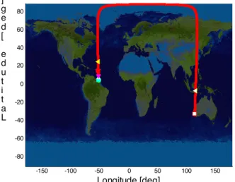
-150 -100 -50 0 50 100 150 -80 -60 -40 -20 0 20 40 60 80 Longitude [deg] L a t i t u d e [ d e g ]
Figure 1: Ground track of the simulated trajectory, obtained with the quaternion scheme
Figure 1 presents the ground track of the simulated trajectory, obtained with the quaternion scheme. Figure 2 presents a the superposition of the speed, the flight-path heading and inclination, the longitude, the latitude and the altitude of the launcher as function of the flight time obtained with each scheme. The graphics of Figure 2 show the three schemes produce a pretty similar trajectory. For the six presented variable, the difference is negligible, less than 1 %.
Section 3: Computation time and In-depth Analysis
As stated in section 1, the equations of each scheme are quite different in their development but also in their use. These differences affect the implementation and computation time of each scheme. The polar coordinates are the easiest one to implement; the differential equations just have to be written into the simulator. There is no further task to be done as all the variables required in the processing are directly available. In the Cartesian approach, the physical values of the radius and of all the angles defining the transfer matrices has to be calculated from the Cartesian states. Then it is possible to compute the forces and transfer matrices to finally write the differential equations. The quaternion approach is similar; the radius, the flight-path speed and, depending of the precision of the Earth model, the latitude and the longitude need to be calculated before being able to compute the external and the fictitious forces, and to
4 implement the differential equations. These supplementary operations increase the computation time of these two schemes. Also, for the Cartesian and quaternion approaches, physical variables need to be calculated from their states to compare their trajectories with the polar one. The graphic of Figure 3 shows the computation time of the quaternion and the Cartesian approaches to be respectively 3.75 times and 2.75 times longer than the polar one. As a point of comparison, the polar approach lasts 1.4852 s on a 2 GHz Intel® T3200 processor. The difference in computation time between the quaternion and Cartesian schemes can be explained by the fact that the mathematical operations on quaternion are harder and therefore longer than their equivalent on vectors.
a) Speed b) Flight-path heading
0 500 1000 1500 2000 2500 3000 -40 -20 0 20 40 60 80 100 Time [s] L a t i t u d e [ d e g ] c) Latitude 0 500 1000 1500 2000 2500 3000 -20 0 20 40 60 80 100 Time [s] F l i g h t -p a t h I n c l i n a t i o n [ d e g ] d) Flight-path inclination 0 500 1000 1500 2000 2500 3000 -100 -50 0 50 100 150 Time [s] L o n g i t u d e [ d e g ] e) Longitude 0 500 1000 1500 2000 2500 3000 -200 0 200 400 600 800 1000 Time [s] A l t i t u d e [ k m ] Quaternion Polar Cartesian f) Altitude Figure 2: Superposition of the simulations with the three schemes
Also, the polar and the quaternion approaches cannot be used for the whole launch as they have discontinuities. Mainly the discontinuity of the flight-path inclination at 90˚ will cause problems at the beginning of the launch when the launcher is in its vertical ascent phase. The polar coordinates can be approximated by a vertical polar scheme, see Marrdonny and Mobed[5] but, in this approximation, it is impossible to add the thrust orientation angles (σ and ε); the pitch-over maneuver cannot be done with this approximation. These discontinuities make the Cartesian approach the only one which is suitable for the whole launch. As the atmospheric part of the launch is nearly never guided[6], the model does not need to
5 be able to predict the states of the launcher in this part, the discontinuity discussed in this paragraph is not relevant outside the vertical ascent phase. Therefore, regarding guidance law, this discontinuity should not interfere in the analysis of the schemes.
However, the discontinuity when the launcher passes over the poles can be, in high inclination orbits, a problem for the guidance algorithm. This pass will occurs during the guided exo-atmospheric phase. Hence, regarding the discontinuity at the poles, the choice of polar coordinates appears risky.
Quaternion Polar Cartesian
0 0.5 1 1.5 2 2.5 3 3.5 4 R e l a t i v e C o m p u t a t i o n T i m e
Figure 3: Comparison of the computation time
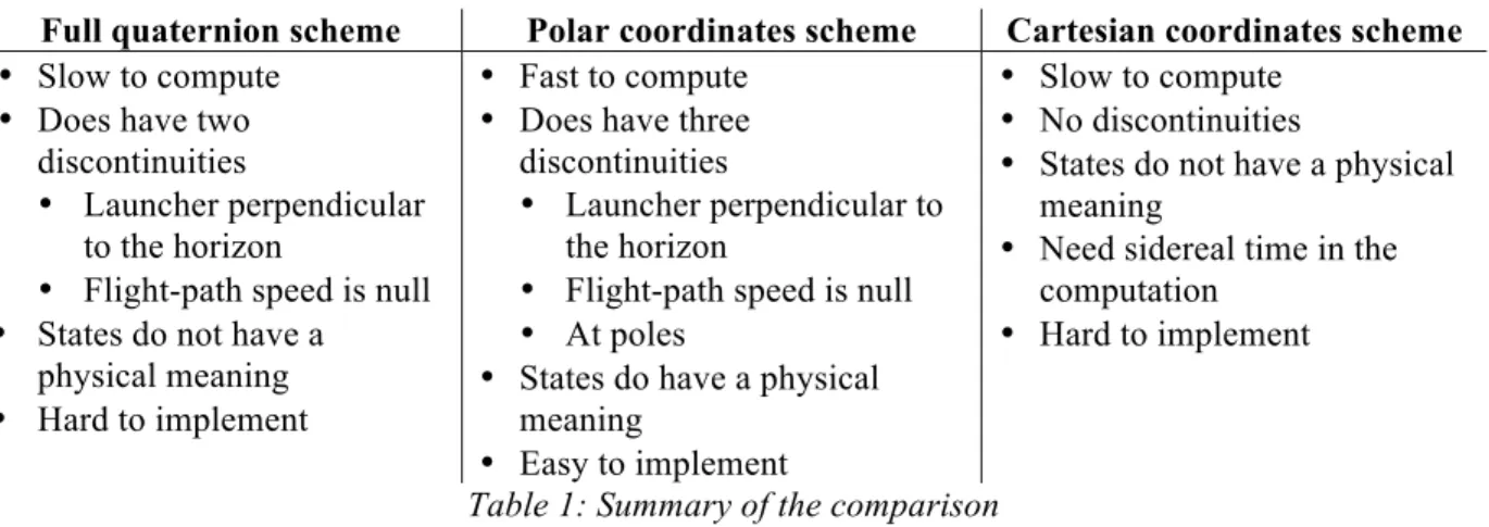
The Table 1 summarizes all these previous comparisons.
Full quaternion scheme Polar coordinates scheme Cartesian coordinates scheme
• Slow to compute • Does have two
discontinuities
• Launcher perpendicular to the horizon
• Flight-path speed is null • States do not have a
physical meaning • Hard to implement
• Fast to compute • Does have three discontinuities
• Launcher perpendicular to the horizon
• Flight-path speed is null • At poles
• States do have a physical meaning
• Easy to implement
• Slow to compute • No discontinuities
• States do not have a physical meaning
• Need sidereal time in the computation
• Hard to implement
Table 1: Summary of the comparison
Conclusion
This paper presents a comparison between three schemes for the translation equations of motion of a launcher: one based on polar coordinates, one based on Cartesian coordinates and one using a full quaternion. The second section showed the accuracy of the three schemes is similar. In the first and third sections, comparisons on inherent characteristics and on computation time show major differences between the three schemes.
The polar coordinates scheme seems best suited for exo-atmospheric guidance. It is the quickest to compute and the easiest to visualize and understand. However, it should not be used around the discontinuity at the poles. A protection to switch to Cartesian scheme, the approach with no discontinuity, when the launcher get close to it should be included.
6
Acknowledgement
The authors would like to thank the Natural Sciences and Engineering Research Council of Canada (NSERC), Numérica Technologies Inc. and the Fonds Québécois de Recherche sur la Nature et les Technologies (FQRNT). Their financial support has made this work possible. We would also like to thank Defence Research and Development Canada (DRDC) who initiated and supported this project.
References
[1] Blakelock, John H. Automatic Control of Aircraft and Missiles. 2nd edition. John Wiley & Sons, Inc.,
1991.
[2] Zipfel, Peter H. Modeling and Simulation of Aerospace Vehicle Dynamics Second Edition. 2nd
Edition. AIAA Education Series, 2007.
[3] Tewari, Ashish. Atmospheric and Space Flight Dynamics. Birkhäuser Boston, 2007.
[4] Vachon, Alexandre, André Desbiens, Eric Gagnon, and Rocco Farinaccio. "Equations of Motion of a
Launcher Using a Full Quaternion." 20th AAS Space Flight Mechanics Meetings. 2010.
[5] Marrdonny, Mohamadd, and Mohammad Mobed. "A Guidance Algorithm for Launch to Equatorial
Orbit." Aircraft Engineering and Aerospace Technology 81, no. 2 (2009): 137-148.
[6] Dukeman, Gregory A. Closed-Loop Nominal and Abort Atmospheric Ascent Guidance for
Rocket-Powered Launch Vehicles. PhD Thesis, Georgia Institute of Technology, 2005.
7
Appendix B: Polar Equations