Multi-scale navigation of large trace data: A survey

Titre:

Title

: Multi-scale navigation of large trace data: A survey

Auteurs:

Authors

: Naser Ezzati-Jivan et Michel R. Dagenais

Date: 2017

Type:

Référence:

Citation

:

Ezzati-Jivan, N. & Dagenais, M. R. (2017). Multi-scale navigation of large trace data: A survey. Concurrency and Computation: Practice and Experience, 29(10),

p. 1-20. doi:10.1002/cpe.4068

Document en libre accès dans PolyPublie

Open Access document in PolyPublie

URL de PolyPublie:

PolyPublie URL: https://publications.polymtl.ca/2980/

Version: Version finale avant publication / Accepted version_{Révisé par les pairs / Refereed} Conditions d’utilisation:

Terms of Use: Tous droits réservés / All rights reserved

Document publié chez l’éditeur officiel

Document issued by the official publisher

Titre de la revue:

Journal Title: Concurrency and Computation: Practice and Experience

Maison d’édition:

Publisher: Wiley

URL officiel:

Official URL: https://doi.org/10.1002/cpe.4068

Mention légale:

Legal notice:

This is the peer reviewed version of the following article: Ezzati-Jivan, N. & Dagenais, M. R. (2017). Multi-scale navigation of large trace data: A survey. Concurrency and Computation: Practice and Experience, 29(10), p. 1-20, which has been published in final form at 10.1002/cpe.4068. This article may be used for non-commercial purposes in accordance with Wiley Terms and Conditions for Self-Archiving.

Ce fichier a été téléchargé à partir de PolyPublie, le dépôt institutionnel de Polytechnique Montréal

This file has been downloaded from PolyPublie, the institutional repository of Polytechnique Montréal

Multi-scale Navigation of Large Trace Data: A Survey

Naser Ezzati-Jivan

Department of Computer and Software Engineering

Ecole Polytechnique Montreal Montreal, Canada

n.ezzati@polymtl.ca

Michel R. Dagenais

Department of Computer and Software Engineering

Ecole Polytechnique Montreal Montreal, Canada

michel.dagenais@polymtl.ca

ABSTRACT

Dynamic analysis through execution traces is frequently used to analyze the runtime behavior of software systems. However, tracing long running executions generates volu-minous data, which is complicated to analyse and manage. Extracting interesting performance or correctness character-istics out of large traces of data from several processes and threads is a challenging task. Trace abstraction and visu-alization are potential solutions to alleviate this challenge. Several efforts have been made over the years in many sub-fields of computer science for trace data collection, main-tenance, analysis, and visualization. Many analyses start with an inspection of an overview of the trace, before dig-ging deeper and studying more focused and detailed data. These techniques are common and well supported in geo-graphical information systems, automatically adjusting the level of details depending on the scale. However, most trace visualization tools operate at a single level of representation, which is not adequate to support multi-level analysis. So-phisticated techniques and heuristics are needed to address this problem. Multi-scale (multi-level) visualization with support for zoom and focus operations is an effective way to enable this kind of analysis. Considerable research and several surveys are proposed in the literature in the field of trace visualization. However, multi-scale visualization has yet received little attention. In this paper, we provide a sur-vey and methodological structure for categorizing tools and techniques aiming at multi-scale abstraction and visualiza-tion of execuvisualiza-tion trace data, and discuss the requirements and challenges faced in order to meet evolving user demands.

1.

INTRODUCTION

Software comprehension is the process of understanding of how a software program behaves. It is an important step for both software forward and reverse engineering, which facili-tates software development, optimization, maintenance, bug fixing, as well as software performance analysis [1]. Soft-ware comprehension is usually achieved by using static or dynamic analysis [2].

Static analysis refers to the use of program source code and other software artifacts to understand the meaning and func-tion of software modules and their interacfunc-tions [3]. Although the software source codes and documents can be useful to understand the meaning of a program, there are situations where they are not very helpful. For instance, when the documents are outdated, they may not be very useful. Sim-ilarly, a rarely occurring timing related bug in a distributed system may be very difficult to diagnose by only examining the software source code and documents.

Dynamic analysis, on the other hand, is a runtime anal-ysis solution emphasizing dynamic data (instead of static data) gathered from program execution. Dynamic analysis records and examines the program’s actions, logs, messages, trace events, while it is being executed. Dynamic analysis is based on the program runtime behavior. This information is usually obtained by instrumenting the program’s binary or source code and putting hooks at different places (e.g., entry and exit points of each function) [1, 4]. However, there are other ways to dynamic analysis as well, for instance, VTune [5] and HPCToolkit [6] are two examples of sampling-based performance tools that add no instrumentation.

The use of dynamic analysis (through execution traces) to study system behavior is increasing among system adminis-trators and analysts [7, 8, 9]. Tracing can produce precise and comprehensive information from various system levels, from (kernel) system calls [10, 11, 12] to high-level architec-tural levels [13], leading to the detection of more faults, (per-formance) problems, bugs and malwares than static analysis [14].

Although dynamic analysis is a useful method to analyze the runtime behavior of systems, this brings some formidable challenges. The first challenge is the size of trace logs. They can quickly become very large and make analysis difficult [15]. Tracing a software module or an operating system may generate very large trace logs (thousands of megabytes), even when run for only a few seconds. The second challenge is the low-level and system-dependent specificity of the trace data. Their comprehension thus requires a deep knowledge of the domain and system related tools [10].

In the literature, there are many techniques to cope with these problems: to reduce the trace size [12, 2], compress trace data [16, 4], decrease its complexity [17], filter out the useless and unwanted information [11] and generate high

level generic information [18]. Visualization is another mech-anism that can be used in combination with those techniques to reduce the complexity of the data, to facilitate analysis and thus to help for software understanding, debugging and profiling, performance analysis, attack detection, and high-lighting misbehavior while associating it to specific software sub-modules (or source code) [19, 20, 21].

Even using trace abstraction and visualization techniques, the resulting information may still be large, and its analy-sis complex and difficult. An efficient technique to alleviate this problem is to organize and display information at dif-ferent levels of detail and enable some hierarchical analysis and navigation mechanism to easily explore and investigate the data [22, 23]. This way, multi-scale (multi-level) vi-sualization, can enable a top-down/bottom-up analysis by displaying an overview of the data first, and letting users go back and forth, as well as up and down (focus and zoom) in any area of interest, to dig deeper and get more detailed information [24, 25].

Of the many different trace visualization tools and tech-niques discussed in the literature [26, 20, 27, 3] and among those few interesting surveys on trace abstraction and vi-sualization techniques [19, 15, 1], only a small fraction dis-cusses and supports multi-level visualization. This moti-vated the current survey, to discuss and summarize the tech-niques used in multi-level visualization tools and interfaces (whether used for tracing, spatial tools, online maps, etc.) and the way to adapt those solutions to execution trace anal-ysis tools.

Indeed, constructing an interactive scalable multi-level vi-sualization tool, capable of analyzing and visualizing large traces and facilitating their comprehension, is a difficult and challenging task. It needs to address several issues. How to generate a hierarchy of abstract trace events? How to orga-nize them in a hierarchical manner, helping to understand the underlying system? How to visualize and relate these events in various levels with support of appropriate LOD (Level of Details) techniques?

Although the techniques discussed in this paper are generic and applicable to any trace data, our focus will be more on the area of operating system (kernel) trace data and anal-ysis, when this distinction is relevant. Kernel traces have some specific features that differentiate them from appli-cation (user) level traces. For example, there is mostly a discontinuity between the execution of events for a process, because of preemption and CPU scheduling policies. An-other example is, unlike An-other (e.g., user-level) tracers that monitor only one specific module or process, kernel traces usually contain events from different modules (disk blocks, memory, file system, processes, interrupts, etc.), which may complicate the analysis.

The paper is structured as following. First, we discuss the techniques to generate multiple levels of trace events from the original logs, focusing on kernel trace data. Secondly, we present a taxonomy for multi-scale visualization methods targeting hierarchical data, looking at the existing trace vi-sualization tools. Then, we study various solutions to model the hierarchical data. Finally, this paper will conclude with

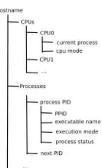
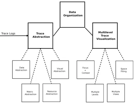
a summary and outline for future work. Figure 1 depicts the topics investigated in this paper.

2.

MULTI-LEVEL TRACE ABSTRACTION

TECHNIQUES

As mentioned earlier, execution traces can be used to an-alyze system runtime data to understand its behavior and detect system bottlenecks, problems and misbehaviors [7, 8]. However, trace files can grow quickly to a huge size which makes the analysis difficult and cause a scalability problem. Therefore, special techniques are required to reduce the trace size and its complexity, and extract meaningful and useful information from original trace logs.

In the literature, various trace abstraction techniques are surveyed, including two recent systematic surveys [1, 2]. Here, we present a different taxonomy of trace abstraction techniques, based on their possible usages in a multi-level visualization tool.

We categorize trace abstraction techniques into four major categories: 1- Content-based (data-based) abstraction tech-niques, those based on the content of events. 2- Metric-based abstraction, the techniques to aggregate the trace data based on some predefined metrics and measures. 3- Visual abstrac-tion, the techniques mostly used in the visualization steps. 4- Resource abstraction techniques, those techniques about extracting and organizing the resources involved within trace data.

2.1

Content-based (data-based) Abstraction

Using the events content to abstract out the trace data is called content-based abstraction or data-based abstraction. Data-based abstraction can be used to reduce the trace size and its complexity, generalize the data representation, group similar or related events to generate larger compound events, and aggregate traces based on some (predefined) metrics. In the following, we study all of these content-based abstraction techniques.

Trace Size Reduction

In the literature, various techniques have been developed to deal with the trace size problem: selective tracing, sampling, filtering, compression, generalization and aggregation. Selective tracing [9] refers to trace only some selected mod-ules/processes of the system, or gather only the interesting behavior, instead of the whole system. Abstract execution [28] is one of the selective tracing techniques. It stores only a small set of execution trace events for later analysis. Once needed, for any area of interests, this technique re-generates a full trace data by re-executing the selected program mod-ule. Shimba [3], a trace visualization tool, also uses a selec-tive tracing method. LTTng Linux kernel tracer [29] can be configured to trace only the requested modules, say network, file system, etc, instead of tracing the whole operating sys-tem, resulting in a reduced amount of collected trace data which is useful and important for an efficient postmortem analysis.

Instead of processing all events, trace sampling selects and inspects only a variety of events from the trace data. Trace

Figure 1: Taxonomy of topics discussed in this paper.

sampling is used in [30], [31], [32] and [33] and also in AVID visualization tool [26]. STAT (Stack Trace Analysis Tool) [34] is a scalable debugging tool that targets very large scien-tific applications. STAT processes the stack traces gathered during a sampling time to build a call graph prefix tree to extract and group common behavior classes within the pro-gram runtime space. In addition to sampling at the time of postmortem analysis, trace size reduction can be also done via sampling events at the time of measurement [35]. Since sampling filters trace events in an arbitrary manner, it may lose information and not preserve the actual system behav-ior.

Trace filtering is the removal of all redundant and unnec-essary events from the trace events, highlighting the events that have some pre-specified importance. Filtering can be done based on various criteria such as event timestamp, event type, event arguments, function name, process name, class or package name, and also the priority and importance of events [36, 37]. For example, an analyst may keep only the events related to socket and network operations and fil-ter the rest out when he/she works only on the network behavior analysis. Fadel et al. [11] use filtering in the con-text of kernel traces to remove memory management events (out of analysis scope events) and page faults (noises) from the original data.

Trace compression is another technique used to reduce the trace size. It works by storing the trace events in a compact form by finding similarities and removing redundancies be-tween them [4]. Compression has two common forms: lossy compression that may discard some parts of the source data (e.g., used in video and audio compression) and lossless com-pression that retains the exact source data (e.g., used in ZIP file format). Kaplan et al. [16] studied both lossy and loss-less compression techniques for memory reference traces and proposed two methods to reduce the trace size by

discard-ing useless information [16]. The drawback is that the com-pression technique cannot be used much for trace analysis purposes. Indeed, compression is more a storage reduction technique rather than an analysis simplification technique. Moreover, since trace compression is usually applied after generating trace events and storing them in memory or disk, it is not applicable for online trace analysis, when there is no real storage for all live trace events.

Event Generalization

Being dependent on a specific version of the operating sys-tem or particular version of tracer tool can be a weakness for the trace analysis tools. Generalization is one solution to this problem: the process of extracting common features from two or more events, and combining them into a gen-eralized event [38]. Generalization can be used to convert the system related events into more generalized events. Es-pecially in Linux, many system calls may have overlapping functionality. For example, the read, readv and pread64 system calls in Linux may be used to read a file. However, from a higher level perspective, all of them can be seen as a single read operation. Another example is generalizing all file open/read/write/close events to a general “file oper-ation” event in the higher levels [10]. PAPI interface [39] abstracts hardware specific events to a set of general and derived events (such as ratios of native and preset events and integration of events with system parameters). Using this interface users can dynamically specify the new derived events to be used in postmortem analysis and modelling.

Event Grouping and Aggregation

Trace aggregation is one of the critical steps for enabling multi-scale analysis of trace events, because it can provide a high-level model of a program execution and ease its compre-hension and debugging [40]. In the literature, it is a broadly used method to reduce the size and complexity of the traces, and generate several levels of high level events [41, 11, 40,

42, 12, 18]. In essence, trace aggregation integrates sets of related events, participating in an operation, to form a set of compound and larger events, using pattern matching, pat-tern mining, patpat-tern recognition and other techniques [42]. For instance, Fadel et al. [11] used pattern matching to aggregate kernel traces gathered by the LTTng Linux ker-nel tracer [29]. Since trace data usually contain entry and exit events (for function calls, system calls, or interrupts), it is then possible to find and match these events and group them to make aggregated events, using pattern matching techniques. For example, they form a “file read” event by grouping the “read system call” entry and exit events [11], and some possible file system events between these two (Fig-ure 2). A similar technique is exploited by [14] to group function calls into logically related sets, but in user-space level.

By using a set of successive aggregation functions, it is pos-sible to create a hierarchy of abstract events, in which the highest level reveals more general behaviors, whereas the lowest level reveals more detailed information. The highest level can be built in a way that represents an overview of the whole trace. To generate such high level synthetic events, it is required to develop efficient tools and methods to read trace events, look for the sequences of similar and related events, group them, and generate high level expressive syn-thetic events [42, 43].

Figure 2: Recovering a “file read” event from trace events.

Source [11]

Wally et al. [12] used trace grouping and aggregation tech-niques to detect system faults and anomalies from kernel traces. However, their focus was on creating a language for describing the aggregation patterns (i.e., attack scenarios). Both proposals [11, 12], although useful for many examples of trace aggregation and for applications to the fault identi-fication field, do not offer the needed scalability to meet the demands of large trace sizes. Since they use disjoint pat-terns for aggregating the events, for large traces and for a large number of patterns, it will be a time-consuming task to take care all of patterns separately. Further optimization work is required in order to support large trace sizes and a more efficient pattern processing engine [18].

Matni et al. [17] used an automata-based approach to de-tect faults like “escaping a chroot jail” and “SYN flood at-tacks”. They used a state machine language to describe the attack patterns. They initially defined their patterns in the SM language and using the SMC compiler [44]. They were able to compile and convert the outlined patterns to C lan-guage. The problem with their work is that the analyzer is not optimized and does not consider common information sharing between patterns. Since their patterns mostly ex-amine events belonging to a small set of system processes and resources, it would be possible to share internal states between different but related patterns. Without common shared states, patterns simply attempt to recreate and compute those shared states and information, leading to re-duced overall performance. Also, since preemptive schedul-ing in the operatschedul-ing system mixes events from different pro-cesses, the aforementioned solutions cannot be used directly to detect complex patterns, because of the time multiplexing brought by the scheduler. It needs to first split the events sequences for the execution of each process and then apply those pattern matching and fault identification techniques. These problems were addressed in our previous work [10, 18]. We proposed a stateful synthetic event generator in the context of operating system kernel traces. An efficient trace aggregation method is designed for kernel traces consider-ing all kernel specific features (extractconsider-ing execution path, considering scheduling events, etc). The work shows that sharing the common information simplifies the patterns, re-duces the storage space required to retain and manage the patterns, increases the overall computation efficiency, and finally reduces the complexity of the trace analysis (Figure 3).

Figure 3: Trace aggregation time comparisons for stateful and stateless approaches [18].

Pattern mining techniques are also used to aggregate traces and extract high level information from trace logs [45]. It is used to find the patterns (e.g., system problems) that are frequently occurring in the system. Several pattern mining techniques have been studied in [46]. Han et al. [47] clas-sified the pattern mining techniques into correlation min-ing (discovery of correlation relationships), structured pat-tern mining (similarity indexing of structured data), sequen-tial pattern mining (mining of subsequent or frequently oc-curring ordered events), frequent pattern-based clustering (computing frequently occurring patterns in any subsets of high-dimensional data), and associative classification

(dis-covery of different association between frequent patterns); they described several applications for each category. They reported that frequent pattern mining can lead to the dis-covery of interesting associations between various items, and can be used to capture the underlying semantics in input data.

Pattern mining may also be used to find system bugs and problems through mining live operating system trace logs as applied by Xu et al. [8] and LaRosa et al. [7]. LaRosa et al. [7] developed a kernel trace mining framework to detect ex-cessive inter-process communication from kernel traces gath-ered by LTT and dTrace kernel tracers. They used a fre-quent itemset mining algorithm by dividing up the kernel trace events into various window slices to find maximal fre-quent itemsets. Using this technique, they were able to de-tect the excessive inter-process interaction patterns affecting the system’s overall performance [7]. Similarly, they also could find the denial of service attacks by finding processes which use more system resources, and have more impact on the system performance. However, their solution cannot be used to find (critical bug) patterns that occur infrequently in the input trace.

Although pattern-based approaches are used widely in the literature, they face some challenges and have some limita-tions, especially for use in the kernel trace context. Effi-cient evaluation of patterns has been studied in several ex-periments [48, 49]. Productive evaluation of the specified patterns is closely related to multiple-query optimization in database systems [49] that identifies common joins or filters between different queries. These studies are based on iden-tification of sub-queries that can be shared between distinct concurrent queries to improve the computational efficiency. The idea of sharing the joint information and states has also been deployed by Agrawal et al. [48]. They proposed an automaton model titled ”N F Ab_{” for processing the event}

streams. They use the concept of sharing execution states and storage space, among all the possible concurrent match-ing processes, to gain efficiency. This technique is also used in the context of kernel trace data to share the storage and computation between different concurrent patterns [18].

2.2

Metric-based Abstraction

Besides the grouping of trace events and generation of com-pound events, used to reduce the trace size and its complex-ity, another method is to extract some measures and aggre-gated values from trace events, based on some predefined metrics. These measures (e.g., CPU load, IO throughput, failed and successful network connections, number of attack attempts, etc.) may present an overview of the trace and can be used to get an insight into what is really happening in the (particular portion of) trace, in order to find possible underlying problems.

Bligh et al. [50], for instance, show how to use the statis-tics of system parameters to dig into the system behavior and find real problems. They use kernel traces to debug and discover intermittent system bugs like inefficient cache utilization and poor latency problems. Trace statistics, to analyze and find system problems, have been also used in [8, 51, 52]. Xu et al. [8] believe that system level performance indicators can denote the high-level application problems.

Cohen et al. [52] established a large number of metrics such as CPU utilization, I/O request, average response times and application layer metrics. They then related these metrics to the problematic intervals (e.g., periods with a high av-erage response time) to find a list of metrics that are good indicators for these problems. These relations can be used to describe each problem type in terms of atypical values for a set of metrics [51]. They actually show how to use statistics of system metrics to diagnose system problems; However, they do not consider scalability issues, where the traces are too large, and storing and retrieving statistics is a key challenge.

Ezzati et al. [53] proposed a framework to extract the impor-tant system statistics by aggregating kernel traces events. The following are examples of statistics that can be ex-tracted from a kernel trace [53, 54]:

• CPU used by each process, proportion of busy or idle state of a process.

• Number of bytes read or written for each/all file and network operation(s), number of different accesses to a file.

• Number of fork operations done by each process, which application/user/process uses more resources. • The number (or area) of disk is mostly used, the

la-tency of disk operations, and the distribution of seek distances.

• The network IO throughput, the number of failed con-nections.

• The memory usage of a process, the number of (pro-portion of) memory pages are (mostly) used.

To perform metric-based abstraction, a pattern of events is registered for each metric (i.e., a mapping table). Each pattern contains a set of events and an aggregation func-tion identifying how to compute the metric values from the matching trace events. For example, the pattern of a metric like process IO throughput includes all corresponding file read and write events as well as a SUM function (as the aggregation function). The trace abstraction module uses these patterns to inspect the events and aggregate them for all predefined metrics.

Most visualization tools support metric-based abstraction, Vampir [24], Jumpshot[27], TuningFork [21], etc. In these tools, the statistics gathered by metric-based abstraction are displayed as histograms or counts (or average, min, max, etc.), and usually rendered as the highest level of the data hierarchy to show an overview of the underling trace.

2.3

Visual Abstraction

Data abstraction, as explained in the previous section, mostly deals with the data content and does not usually have a sense of the visualization environment. When displaying a large trace set, it may not be possible to visualize all abstract trace events together, because of the limited screen display area. It is sometimes required to perform separately a visual

abstraction of trace data, to aggregate the data and display a small set of events, enabling a simpler and more usable view. Applying different types of visual abstraction, like filtering some unimportant items, grouping and aggregating related events (related rectangles), displacement, simplification, ex-aggeration, or reducing or enlarging the size and shape of events, may reduce the visual complexity of the trace, in-crease its readability and clarity, and sometime improve the performance of graphical rendering of the trace items [55]. While data abstraction is based on analyzing and manip-ulating the trace content, visual abstraction is more about manipulating the trace representation (and not the data it-self) [23]. Many visualization tools use colors and shapes as the elementary elements to represent the trace events. Trace Compass and LTTV [56] use colors to differentiate the var-ious states (waiting, system call, user space, etc.) extracted from trace events. Rectangles are usually used to represent the abstract events and states. In the same way, arrows are used to represent the communication and message passing between different modules (processes). In the LTTV and Trace Compass visualization tools [56], for example, when there is more than one trace event in an area smaller than a pixel, a black dot is shown instead of those events. Annotation is another way to visually abstract the trace items. Annotation can be used to describe a group of events, to display user comments about a trace section, or the con-tent of a message passed between different resources [57]. Labels, as a specific type of annotation, is also used in dif-ferent visualization tools. Ovation [58], the Google chrome tracing tool [59] and Trace Compass [56] use labels to repre-sent function names, system calls, return values, etc. Labels can be also filtered, shortened, enlarged or aggregated when there is more or less display area available [43].

2.4

Resource Abstraction

Trace events are usually multi-dimensional in nature and in-clude interactions of different resources (dimensions). There may be a large number of resources (processes, files, CPUs, memory pages, ...) about which a tracer gathers informa-tion. For instance, a “file open” trace event may contain information from the running process, the file that has been opened, the current scheduled CPU for this operation and the return value (i.e., file descriptor (fd) of the file). There-fore, the abstraction of the resources, and their represen-tation, can also be important to reduce the complexity of the trace display. Grouping resources [25, 41], filtering of uninteresting resources [60], or hierarchical organization of resources [61, 53, 62] are the related techniques used in the reviewed literature.

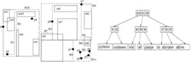
Montplaisir et al. [61] exploited a tree representation (called attribute tree) to organize resources extracted from trace events. One important feature of their work is extracting the resources dynamically from traces. It may also be pos-sible to statically define and organize all existing system re-sources (all classes, all packages, all processes, all files, etc.). However, since the trace data may contain events and in-formation for only a small number of resources, defining the resources statically and in advance will be a waste of time and display space (Figure 4).

Figure 4: Hierarchical abstraction of resources ex-tracted from trace events.

Another representation of resources extracted from trace events is presented in [53, 62]. In their work, a hierarchy is defined for each resource type (also called domain), e.g., one hierarchy for processes, one for files, etc., and the metrics are defined between these domains. They present solutions for constructing cubes of trace data to be used later in trace OLAP (OnLine Analytical Processing) analysis.

Schnorr et al. [25] group the threads based on their asso-ciated processes and then by machine name, cluster and so on. Automatic clustering of system resources is performed in [41]. Two approaches were used: automatic clustering of processes based on their runtime inter-process tion intensity, and combining the inter-process communica-tion informacommunica-tion and the informacommunica-tion of processes extracted from static source code [41].

2.5

Applications of Trace Abstraction

Tech-niques

As explained, trace abstraction techniques are used to re-duce the size and complexity of trace logs to make their analysis simple and more straightforward. One direct appli-cation, for trace reduction and simplifiappli-cation, is system be-havior understanding and comprehension [1]. Other applica-tions are security problems detection (e.g., network attacks), system problems investigation (e.g., performance degrada-tion), comparisons of system execution, monitoring, etc. Beaucamps et al. [63] propose a method for malware de-tection, using abstraction of program traces. They detect malware by comparing the aggregated events to a reference set of malicious behaviors. Uppuluri [38] uses a pattern matching approach to diagnose system problems. In [64], [65] and [66] similar techniques are also used to detect sys-tem problems and attacks. They mainly differ in describ-ing and representdescrib-ing the patterns. STATL [64] models use signatures in the form of state machines, while in [65] sig-natures are expressed as colored petri nets (CPNs), and in MuSigs [66] directed acyclic graphs (DCA) are used to rep-resent the security specifications. Chun Yuan et al. [67] provides an abstraction of system trace events by means of statistical learning technique and classifying system call se-quences to automatic identification of root-causes of known problems (such as page loading error in Internet Explorer web browser).

network problems, and attacks, by looking for fault and at-tack patterns and scenarios in execution traces. Using this method, users can discover problems like inefficient CPU scheduling, network attack attempts, slow disk accesses, lock contention, inappropriate latency, non-optimal memory and cache utilization, and uncontrolled sensitive file modifica-tions [50, 17, 8]. The techniques used in pattern-based fault identification tools resemble the attack discovery techniques in intrusion detection systems (IDS). Intrusion detection sys-tems analyze network packets and look at their payload to find and detect attack signatures. Similar to IDS systems, trace analysis tools, upon detecting such a problematic pat-tern, may generate an alarm or even trigger an automatic response (e.g., killing a process, rebooting the system, etc.) [68].

One of the other techniques to reduce trace complexity and improve understanding is visualization. A proper visual-ization, specially multi-scale visualvisual-ization, can significantly help to alleviate big data analysis problems, as investigated in the next section.

3.

MULTI-LEVEL

TRACE

VISUALIZA-TION

After creating a hierarchy of events, using various abstrac-tion techniques, it is important to have a proper visual-ization model to store and display the hierarchy of events, including a proper navigation and exploration mechanism. Without such a visualization model, displaying large traces may become overly complex, leading to information over-load [69]. In this section, we focus on multi-level visual-ization techniques and tools, and investigate the different techniques for displaying and visually organizing the hierar-chical trace data.

3.1

Hierarchy Visualization Techniques

In the literature, there are many techniques to visualize large hierarchical structures. We categorized them into four main groups: space filling, context+focus, multiple levels, and multiple views. In the following, we explain each technique in more detail.

Space Filling Technique

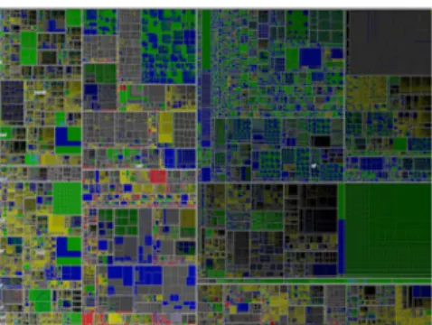
Space filling is a visualization technique used for hierarchi-cal structures which uses almost all available screen space. In this technique, intermediate and leaf nodes are both dis-played as rectangles (or polygons), for which sizes are com-puted based on their importance or property values. One space filling technique is the radial method [70], in which items are drawn radially, the higher levels at the center of the display and lower layers away from the center. Treemap [71] is another popular space filling technique. It allocates the rectangle space of the visible screen to the root node and then splits it among its children based on their properties. In this technique, the rectangle corresponding to each node is labeled with an attribute of that node (size, resource usage, importance, etc). The technique was first used to visualize the directory structure of the file system of a 80MB hard disk [71]. It was later also used to visualize the trace data in Triva visualization tools [25], as well as in Gammatella [72] and LogView [73]. Figure 5 shows the visualization of one million items using the Treemap technique.

Figure 5: Visualization of one million items using treemap.

(source: wikipedia.org)

The main focus of space filling techniques is on the leaf nodes, whereas the non-leaf nodes are not clearly shown. Thus, it can be a candidate for the cases where the leaf-level nodes are of interest and important for analysis (e.g., for presenting unusual patterns at the leaf level). Furthermore, users may loose the focus of the whole system, since it is more difficult to focus on one part, and at the same time keep a global overview. Another problem with this tech-nique is that the small areas (rectangles or polygons) may be difficult to distinguish.

Focus+Context Technique

One problem with the space-filling techniques is that users may loose the position of the visible items, due to the lack of a global overview. Focus+Context techniques solve this problem by simultaneously displaying an overview of the data while also zooming on a small part of the view. In other words, users can zoom and focus on any part of the view, while they see the overall context [74]. One example of this technique is using a magnifier over a text document. You can zoom on any part of the text and enlarge the con-tent by moving the magnifier, while retaining an overview of the data (i.e., the entire page). Tree based visualization techniques are another example of this method, e.g., in a tree based window explorer, you can expand a node to see its content and details, while you see the overview of the data simultaneously.

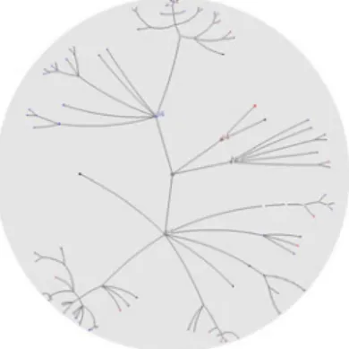
Hyperbolic browser/tree, originally introduced by Lamping et al. [74] exploits a Focus+Context technique. Hyperbolic browser/tree displays the hierarchical data on the hyperbolic space rather than Euclidean space and then maps it to the unit disk, making the entire tree visible at once. In this tree, the focused node is displayed larger, and the degree of interest of other nodes is calculated automatically based on their distances from the selected node. Since the degree of interest for each node is changing with respect to the focused node, the cost of tree redrawing leads to speed concerns. The other problem with this approach is that it cannot display non-hierarchical relationships. Mizoguchi [75] has used the Hyperbolic tree and also machine learning techniques to find the tracks of an intruder in his anomaly detection system. Figure 6 depicts a view of the Hyperbolic technique.

Figure 6: An example of a hyperbolic browser. (source: wikipedia.org)

Multiple-levels Technique

Focus+Context techniques are typically used for displaying and following data sets having clear hierarchies and cate-gories. These techniques display both the context and focus within the same screen, but sometimes, when there is more detailed data for each selected area, it might not be possible to display both the details and the overview on the same display at the same time [76]. One solution for this problem is using various views for displaying the different levels, as often used in online geographical maps.

Two techniques are usually supported in this method. First, semantic zooming [23], in which another semantic level of objects is displayed when changing the zoom level. In a non-semantic zooming approach, as used in many visualiza-tion tools, (TuningFork [21], Jumpshot [27], Trace Compass [56] and Chrome tracing environment [59]), the objects are displayed in larger size as the available display area becomes larger.

The multiple-levels technique usually supports (different types of) linking between the different data layers. To do so, a direct link is kept for different objects (referring), or objects are organized in such a way that relationships can easily be extracted later (matching). Establishing links be-tween different layers enables multi-scale analysis, because it makes possible following one data item within other hier-archy levels.

In the multiple-level techniques, various levels are used to display the different data resolutions, overview on top, and details at the bottom. Users typically see a top-level view and then can zoom and focus on any selected part to get more details [76]. The difference with the Focus+Context approach is that here the views appear separately, not si-multaneously. In other words, more information can be dis-played in this method, because the whole display is used to visualize a view, and there will be no wasted space to show the overview or other data levels. In this method, the trace data is divided, and visualized in various spatial lay-ers. When users zoom, the current view becomes hidden and a completely new view with more detailed data appears (more details and more labels are shown). Supporting se-mantic zooming in this method enables showing more/less information about objects, when users zoom in/out. For

ex-ample, in the highest overview level, only labels of important objects are shown, while in the lowest level, more labels are shown (like in Google maps) [43].

There is a special case of this method called overview + de-tails, used in many visualization tools (Jumpshot [27], Vam-pir [24], Trace Compass [56], etc.), in which the overview and detailed views are shown next to each other (Figure 7). The overview can be the statistics of the important system pa-rameters or only a simple time navigator. Users can browse the overview pane and click on interesting parts to see in another view that section in more details. This method al-lows a simultaneous display of the views. However, it splits the screen and limits the available space for each view [76].

Figure 7: Overivew + Detail method (Trace Com-pass LTTng viewer).

This method shows different data resolutions at different lev-els and lets the user understand and detect the relationships between the different data resolutions intuitively. Although space-usage efficient, and widely used in visualization tools and applications to display large data sets, this method is not exploited much in trace visualization tools. It deserves more consideration, because of its remarkable features.

Multiple Views Technique

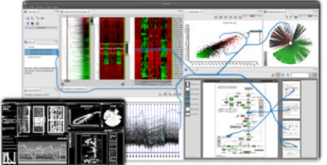
One popular visualization technique, widely used in trace vi-sualization tools, is multiple-views. This technique exploits a flat visualization technique and shows sequentially the dif-ferent aspects of the trace in difdif-ferent (coordinated) views [77].

Using this method, displaying hierarchical data is also pos-sible. It is often implemented as separate views, in which each view displays a separate level. A Primary view is used to show the mainline of the system or an overview of the execution, and a set of auxiliary views display other aspects (or levels), such that selecting an item in one view leads to highlighting corresponding areas in other views [78]. This technique helps users to get a better comprehension through different views. Many trace visualization tools like Zinsight [20], TraceVis [57], Vampir [24], LTTV, Trace Com-pass [56], etc. use coordinated views to display trace ele-ments. The problem with this technique is that users need to simultaneously follow various related views to analyze the system execution, that can be difficult for some users. The views are usually coordinated. Timestamps of events or system resources (e.g., a process name) are used to co-ordinate the views together. For example, when an area is selected in a statistics histogram, all events whose times-tamps are in the range of the selected area will be displayed or highlighted in the events view. Also, when a process is selected in the control flow diagram, all events belonging to this process will be shown in the events view.

In the same way, to show hierarchical relationships between events at different levels, one possible solution is using im-plicit links between elements at different levels. For example, when an item is selected in one level (view), related events in another level (view) can be highlighted. Trace Visualiza-tion tools typically use event timestamps to link the related data together in the hierarchy. When a high level event is selected in one view, all related events in other views with the same timestamp are highlighted and shown.

Figure 8: Context-preserving visualization of re-lated items and links.

Data Correspondence

One important issue in multi-level visualization is deciding about managing and representing the correspondence be-tween data. Techniques are required to extract, organize and visualize the links between related data at different levels. Supporting data correspondence and multi-level navigation are important features of visualization tools to provide. For instance, when users want to follow and dig into an interest-ing high level entity (e.g., an event displayinterest-ing a performance problem or a network attack), these features can be used. In the focus+context and other tree-based methods, the relations between entities at different levels are normally displayed using a tree-based view (expand/collapse). Such relations are also fairly explicit in space filling techniques. However, in multiple-level views, the detection of relations between data at different levels is less explicit, left to the user intuition. In this technique, it is important to present data in such a way that users can seamlessly navigate and understand the relationships between relevant data. To link events in the multiple-view technique, as explained earlier, two general methods may be used: 1- structure-based linking 2- content-structure-based linking. In the former, the events bounding information (e.g., timestamps) or the sys-tem resources (e.g., process, file, etc.) are used to relate events together. In the latter, data semantics are used to link events from different layers (views), e.g., selecting a “HTTP connection” abstract event in a view results in displaying all related events (e.g., socket create, socket call, socket send, socket receive, socket close and so on) in another detailed view.

The details of the links between events, regardless of their type (e.g., structure or content based), can be extracted stat-ically (in the process of aggregation), or dynamstat-ically using matching techniques. In the former, event links are

gener-ated in advance and stored in a type of index to be used later. In the latter, no linking information is stored in ad-vance, the related events are instead matched dynamically in the visualization phase.

Matching is commonly used in spatial applications using a geometric matching algorithm [79]. This algorithm as-sumes that some attributes of the related objects should be matched. In this technique, semantic attributes, metrics, ge-ometrical and structural information from objects are used, for matching similar objects at different scales [80]. To display the links, besides highlighting the related events, it is sometimes useful to also show lines and arrows between relevant views and items, as investigated by Collins et al. [81], Waldner et al. [82] and Steinberger et al. [83]. Collins and Carpendale [81] introduced VisLink, a visual-ization environment that reorganizes various 2D elements and displays links between them. VisLink is generalized for different visualization techniques like Treemap, Hyperbolic, etc. In VisLink, each graph is represented on a separate plane, and the relationships between these planes are dis-played using edge propagation from one visualization to an-other. The same approach is also used in [84] to effectively present all relevant gene expressions and the relations be-tween them and bebe-tween multiple pathways. Waldner et al. [82] extend visual links to graphically present links between related pieces of items across desktop application windows. Figure 9 shows an example of the VizLink visualization.

Figure 9: Visualization of related items and the links between them.

Steinberger et al. [83] believe that using this links visual-ization technique may lead to hiding valuable information. For solving this problem, they introduced context-preserving visual links [83]. In this approach, the items and the con-necting lines are highlighted, helping to find and discover the related items, but special care is taken to avoid hid-ing valuable content. Indeed, the links are routed along the window borders to avoid obstructing the view of items. This technique is attractive and has clear advantages over tradi-tional visual links. However, it may lead to possible visual interferences. Moreover, the issue of dealing with scalable data sets was not addressed in their work and is likely prob-lematic. In the case of particularly large traces, visualizing the links between events may cost too much, and should be studied carefully. Figure 8 depicts context preserving links

visualization.

In this section, different ways to visualize hierarchical data, popular in trace visualization tools, were investigated. In the next section, we study some existing trace visualization tools, explain the abstraction techniques used, and investi-gate their support for multi-level visualization.

3.2

Visualization Tools

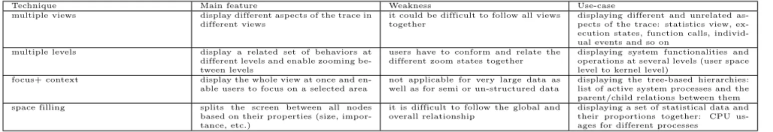
By using an appropriate multi-level visual representation, users can view an overview of the trace, then focus and zoom into areas of interest to get more details. Several stud-ies have been conducted in the area of scalable visualization [15, 20, 85, 22]. In the following, we study various trace visualization tools, from operating system level to applica-tion level tracing, and for each we review the abstracapplica-tion method used, and discuss if they support multi-level visual-ization and the way they handle visualvisual-ization scalability. Vampir [24] is a trace analysis tool used for performance analysis and visualization of MPI (Message Passing Inter-face) programs. Vampir uses the multiple views technique and contains different synchronized views such as global timeline view, process timeline view and communication statistics view. Global timeline is the default view that gets activated automatically when opening a trace. It displays a fine-grained view of the execution behavior. Analysts can then select any individual section of the timeline and zoom to get more detailed information for that part. In addi-tion, users can view statistics (metric based abstraction) for the displayed time interval [86]. Hierarchical visualization is supported using a multi-level space-time (timeline) diagram. In this view, the highest level shows the statistics and there is the possibility of focusing and zooming, where users can explore data for different levels of resources such as cluster, machine, or process. However, the metrics used for repre-senting the system behavior are too low level, and analysts may therefore not understand easily what improvements are possible. A summary of this tool (in conjunction with other tools) is displayed in Table 1.

Similar to Vampir, Jumpshot [27] is a visualization tool for understanding the performance of parallel programs. Jump-shot first displays an overview of the whole trace, and, once the user selects an interval, it displays a detailed view of that interval. The length of time intervals is fixed at each level, and is selected statically or dynamically. Jumpshot uses the SLOG2 trace format [87], a hierarchical file format to handle a large number of events and states in a scalable way, even for large-scale applications. Jumpshot abstracts out the trace events to generate ready-to-display hierarchi-cal preview drawable objects: preview state, preview arrow and preview event. At each detail level, it uses a separate pack degree that shows how many underlying events are used to create the preview objects of the current level. Users can zoom-in and narrow the view to see large intervals and states that were too small in the previous views, but large enough for the current view. Jumpshot supports also resource ab-straction, displaying an aggregated set of processes in a spe-cial view called “mountain range”. The link between views is established based on timestamps. There is no other mecha-nism to directly link the different views and their associated events.

The high-performance computing (HPC) field has developed a rich set of tools and techniques for trace collection, anal-ysis, and visualization. Hardware performance counters, memory traffic, network traffic, call path samples, are some of the data collected by tracing tools in the HPC area. Ex-cept Vampir [24] and Jumpshot [27], there are other great HPC performance analysis tools such as Allinea’s map [88], Intel’s VTune [5], HPCToolkit’s hpctraceviewer [6], TAU [89], and Scalasca [90]. Each of these tools has rich trace collection mechanisms and visualization interfaces. For ex-ample, hpctraceviewer [6] organizes its sampled traces in 3D, where the x-axis is the time, y-axis is is resources, and the depth-axis is the call stack depth. Scalasca [90] organizes its performance data in a CUBE format.

Significant efforts are made in visualizing HPC performance data. Isaacs et al. organize trace data in a logical time or-dering for the ease of understanding performance anomalies [91]. Isaacs et al. [92] provide a rich survey of visualization tools for performance analysis. Landge et al. [93] devised 2D and 3D techniques to visualize the network traffic in mas-sively parallel simulations. Bhatele et al. [94] devised a novel scheme to map performance data from a hardware topol-ogy to an application domain. They use intuitive colouring scheme and weighted arrows to indicate network bottleneck in a tree topology.

AVID (Architecture Visualization of Dynamics in Java Sys-tem) [26] is an Ecplise based offline visualization tool to sum-marize and visualize the object-oriented system’s execution at the architectural level. The diagrams generated by AVID demonstrate the system execution by visualizing the objects and the interactions between them. The system execution is represented by animating the sequences of cells. Each cell denotes the aggregated summary information of the system execution up to that point. A trace sampling method is used to select only a portion of the trace data related to a specific analysis scenario, instead of the whole trace. Even using a sampling method, AVID has scalability issues, and scenarios dealing with large traces cannot be efficiently visu-alized. As mentioned, AVID can be used to understand the system behavior at the architecture level, but it needs the architecture model of the system to be available. This may not always be feasible for all systems. Moreover, it needs a high level model, and the mapping between classes and the architectural entities, to be manually defined by the analyst. However, the analyst is not expected to be familiar with the system architecture [15].

Shimba [3] integrates both static and dynamic information to analyze the behavior of manually selected artifacts of Java applications. Its purpose is not to display a general overview of the system. Using reverse engineering, the static informa-tion including various software artifacts (classes, methods, variables...) are extracted and displayed. Users may then select any interesting component to be traced by Shimba. The resulting trace extracts the interactions between se-lected components and visualizes them using UML sequence diagrams. Shimba uses several abstraction techniques to cope with scalability problems. It generates several levels of abstraction from both static and dynamic information. An example of the former is grouping related software com-ponents to construct higher level entities. An example of

the later is abstracting out the dynamic information, such as sequence diagrams, to higher level diagrams. A pattern matching technique is used to generalize the sequence dia-grams [3]. Unlike other tools that use system-level tracing and then reduce the data, Shimba uses component-level trac-ing, resulting in a small trace data size. It relies on users to select the component that implements a specific feature. However, this is not always possible in a complex system. One problem with this tool is that diagrams are sometimes very large, and thus harder to understand.

Jinsight [95], is an Eclipse based tool for visualization and performance analysis of Java programs. It provides several dynamic views depicting object populations, method calls, thread activities and memory usage. Using an automatic pattern recognition technique, Jinsight can detect repeated behavior patterns from trace data. It uses these patterns to produce an abstract view of the program execution. Jin-sight uses different views to illustrate different aspects of the investigated software behavior. Jinsight supports infor-mation filtering, enabling analysts to filter out uninteresting behaviors. De Pauw et al. [95] showed that the tool was suc-cessful in detecting various problems, such as memory leaks in industrial applications. However, it does not scale well to large traces. Jinsight supports trace aggregation over time in some views.

Ovation [58] is another tool that uses a tree based view called “execution patterns” to visualize execution traces. Similar to Jinsight, it uses automatic pattern recognition to extract and identify patterns of repeated executions. The execution pattern view displays multiple levels of data to users: a high level view first and more details on demand. Ovation firstly shows a generalized view of the system behavior using exe-cution patterns. It supports drill-down, roll-up, zoom and pan operations. Users can zoom and focus on any area of interest to see and find more details in an enlarged view. De Pauw et al. [58] reported that Ovation has been used successfully to detect unexpected execution patterns and to improve performance of large systems. However, Ovation reveals relatively detailed low level (i.e. method-level) infor-mation about the application execution, and assumes that the analyst has enough knowledge of the system to query this information. Furthermore, it works better for single program comprehension, rather than general multi-module systems (like operating system).

Zinsight introduced by De Pauw et al. [20], is a visualization tool that facilitates system comprehension and performance problems detection. It is used to analyze special mainframe software and hardware by examining operating system level trace events. Zinsight provides facilities for creating high level abstract views from the low level execution traces. It uses pattern recognition techniques to discover and extract execution flow patterns from raw events. It supports dif-ferent coordinated views like event flow view, sequence con-text view, statistics view. These linked views help analysts to see the system execution at a higher level of abstraction, and make them able to navigate through different levels. Al-though Zinsight supports trace abstraction and linked views, it has scalability problems and is not able to visualize traces unless they completely fit in main memory [96].

TuningFork [21] was introduced to analyze and visualize traces gathered from the execution of very large realtime systems. They vertically integrate data from multiple levels of abstractions, from hardware and operating system lev-els to the application level, in order to analyze the system. TuningFork also stores coarse-grained summaries of data, enabling navigation across different time scales, from hours to milliseconds, and exploration in multiple levels of granu-larity.

Tracevis [57] is used to visualize Java programs. It uses mul-tiple views to display different aspects of program execution, including timeline and dynamic call graph. Tracevis sup-ports zooming in any selected area to display detailed trace data. Tracevis also supports correlating trace instructions with both the assembly and c code. A multi-level statis-tics view is supported to show different levels of abstrac-tion. Tracevis uses metrics based abstraction and displays the statistics for any selected area by means of annotations. Triva [25] is another tool that aims to visualize the trace events of large parallel applications in a hierarchical manner, supporting visualization scalability. It supports the dynamic hierarchical organization of trace data and uses the Treemap space filling technique to visualize trace data. Triva also supports a hierarchical organization of resources, in which the threads of a process are grouped together, and processes are then grouped by machine, cluster and then grid. In this way, Triva can simultaneously visualize more monitoring entities than other traditional techniques (e.g., space-time), in different time granularity (from microseconds to days) [25].

LTTV (Linux Trace Toolkit Viewer) [56], developed at Dor-sal lab, is another visualization tool that shows events gener-ated by the LTTng kernel tracer [29]. It provides a statistics view, control flow view and event view. The statistics view presents metrics for the different event types. The control flow view displays an overall view of the system execution, aggregated by processes and threads. It supports physical zooming, scrolling and filtering. However, it does not sup-port multi-level trace abstraction and linked events. The same limitation applies to Trace Compass [56] a full-featured Eclipse based LTTng trace viewer, with more views and features and supporting different visual abstraction mech-anisms (e.g., labels, etc).

4.

HIERARCHICAL ORGANIZATION OF

TRACE DATA

A single pass over the trace data is normally sufficient to aggregate the trace and generate high level events to reduce its size, and possibly detect some problems. In multi-level trace visualization, users want to access any arbitrary area of a trace with support for interactive exploration, panning, searching (e.g., interval search, etc.), focusing and zooming. A proper hierarchical modeling of the trace data then be-comes very important for large traces.

Behind the scene of the aforementioned visualization tools and techniques, are the supporting data structures. The first step for building a multi-level visualization tool, and linking events at different levels, is modeling and storing the generated abstract events in such a way that they can easily

T ab le 1 : T rac e v is u al iz at io n t o o ls and the ir fe atu re s. T ra ce Vi su a liza ti o n T o ol Mu lt ip le L ev el s Ab st rac ti o n T y p e Vi su a liza ti o n T y p e d a ta a b st ra ct io n m et ri c-b a sed a b st rac ti o n v isu a l ab st ra ct ion reso u rce a b st ra ct io n sp a ce fi lli n g tec h n iq u e m u lt ip le lev el s m u lt ip le v iews co n tex t + fo cu s V a m p ir 4 fi lt er in g + a gg rega ti on 4 4 4 4 4 A VID m a n u al sa m p lin g a n im at io n m a n u al 4 Ju m p sh o t 4 4 4 4 m o u n ta in ran g e 4 4 S h im b a st a ti c an a ly si s sel ect iv e tr a ci n g an d a b st rac ti o n a gg rega ti on o f se q u en ce d ia gr a m Ji n si g h t 4 rep et it ion d et ect ion 4 4 4 4 O v a ti on 4 rep et it ion d et ect ion 4 4 4 ex ecu ti o n p at ter n s Zi n si gh t 4 rep et it ion d et ect ion 4 a n n ot a ti o n 4 4 ev en t fl o w ev en t ty p e st at ist ics T u n in g F or k 4 4 co lor 4 T ra cev is 4 fi lt er in g 4 a n n ot a ti o n 4 4 T ri v a 4 4 co lor 4 tr eem a p L TTV 4 co lor 4 4 4

be fetched and extracted on demand. For efficient manage-ment of various abstract events, it is required to exploit an optimized data organization in terms of compactness and access efficiency. The data organization should enable both horizontal and vertical analysis in large traces. Horizontal analysis means going back and forth in the trace, inspecting events and processing the data for understanding the trace. Vertical analysis refers to hierarchical and multi-level anal-ysis. In the following, we review different data structures used to model and manage trace events, abstract events and states, and also establish links between them.

Every time users query the system and ask to view the events and information (e.g., statistics of some system parameters), at arbitrary places in the trace, it would be possible but impractically long to reprocess the trace from the starting point, apply the requested trace analysis (abstraction, re-duction, etc.) techniques and get the requested information. The cost of reading and processing the whole trace for each single query, would indeed be too costly for anything but the smallest traces. Indeed, the horizontal analysis aims to support the efficient and scalable analysis of large traces for arbitrary points (and intervals). Users want to jump effi-ciently, without any undue or apparent delay, to any place in the trace to analyze the data to get an insight into the program behavior at that point. The challenge is similar for the vertical analysis.

Some projects use periodic snapshots (at checkpoints) to col-lect and store the intermediate analysis data. This method splits the input trace into equal (or possibly different) du-rations (e.g., a checkpoint for each 100K events) and stores aggregated data at each checkpoint. Later, at interactive analysis time, instead of reading the whole trace, the viewer opens and reads the trace from the nearest previous check-point to the given query check-point and rerun the patterns for this small set of events and regenerates the desired informa-tion. The checkpoint method is used in LTTV (the LTTng trace viewer) and was used initially in Trace Compass [56]. Related to the checkpoint method, LTTngTop, developed by Desfossez et al. [54] at Dorsal lab1, is an efficient command-line tool to index LTTng kernel traces and extract various statistics on the system parameters. It is, to a certain ex-tent, a more detailed and efficient version of the Linux TOP command. It dynamically displays an ongoing state of the system, for continuous time periods, using operating system trace data. LTTngTop aggregates trace events and stores them in different checkpoints to enable navigating through the time axis and producing statistics for any time period, for the current time or any time in the past.

Although the checkpoint method is useful to avoid reading the whole trace for each query, it has some limitations. For instance, it always requires accessing the original trace data. Then, when the original trace data is not available, or if there is not enough space for storing a whole streaming trace, this method cannot be used. Moreover, the snapshots have a fairly constant size while their number increases with the trace duration. There may indeed be a lot of redundancy between the content of snapshots at consecutive checkpoints.

1

http://www.dorsal.polymtl.ca

Some values change frequently while others rarely vary and remain constant from one checkpoint to the next. This does not scale very well for large trace sizes and long durations. In some tools, the snapshots were stored in main memory, forcing a limit on the trace size that they could handle. To solve this problem, Ezzati et al. [53] proposed a dy-namic checkpoint method (different checkpoint intervals for different metrics) to analyze trace events. In their work, each metric uses its own checkpoint interval, based on its precision, degree of granularity and importance. They also avoid storing the whole trace to answer the analysis queries. Queries are served using only a compact trace index, created at trace pre-processing time. Although the solution pre-sented in [53] works well with offline traces and was tested for very large traces, since they store snapshots and trace events at regular-basis periods, the size of data stored be-hind their work grows linearly with the trace size and can become unexpectedly large for long streaming traces. The cube data model [62] was proposed to address this problem for live trace streams of arbitrary size. It enables efficient multi-level and multi-dimensional trace analysis, similar to OLAP analysis in database applications.

Montplaisir et al. [97, 98] introduced a tree-based structure, called “state history tree” to store and query the incremen-tally arriving interval data. They used this data structure to manage and model the system state value changes [61]. Since a tree-based structure is used, they can answer the queries quickly and directly by only traversing the related branches and nodes, without requiring access to the origi-nal trace. The problem with their proposed structure is the large size of the generated tree, which was addressed by the partial history tree [97]. A partial history tree avoids stor-ing all intermediate data in the tree, but requires access to the original trace data during the analysis phase. The par-tial state history reduces the state history tree size by more than a hundredfold for a small increase in query time. In their approach [98, 61], the proposed history tree essentially stores intervals, each interval represents a state value and contains a key, a value and a time interval. Since (raw or abstract) trace events usually have the same content, they can also be modeled and stored as interval data, as is the case for the SLOG file format [87].

Chan et al. [87] proposed a file format called SLOG (and improved later as SLOG2), a hierarchical trace format used to store trace events (called drawable objects in their work) in a R-tree like structure for efficient interactive display. The SLOG file format contains intervals, representing the draw-able objects, and a tree index schema to provide direct access to any address within the file. Each interval is described by bounding times and a thread number. The index tree is like a binary tree that stores the elements in different-size buck-ets. At each level of the tree, the duration of the buckets is the same. In this tree, the root node represents the whole trace length (interval 0 to T). Each node in the second level represents time intervals of size 0+T₂ . The next level shows intervals of size 0+T

4 . In the same way, leaf nodes show

in-tervals that are smaller than or equal to a ∆Tmin. Objects

are stored in the smallest containing node, in both leaf and non-leaf nodes.

At display time, for any given time t, only the intervals intersecting with t will be read and displayed. Using this file format, Chan et al. [87] reported that they could achieve nearly constant access time for different time intervals. The main problem with their work is that they use the same time durations to store the drawable items. For the cases where trace events are not uniformly distributed along the time axis, some nodes will be full and others almost empty. This may affect the access time and give different access times for different locations in the trace. This solution models the different drawable objects (events, states and so on) but does not consider the links and the relations between objects. Their file format has been used in Jumpshot [27]. Modeling trace events as interval data, and using interval management structures to store the trace events, appears to be a good solution for very large traces.

There are many other interval management structures that could be used as storage for trace events. The segment-tree is a basic data structure used for storing the line segments. It is a balanced binary tree where each node is defined by its bounding box. In this tree, leaf nodes represent the el-ementary segments in an ordered way, and non-leaf nodes correspond to the intervals that are union of the underlying children’s intervals. The interval duration of each node is approximately half the interval of its parent node. Figure 10 shows an example of a segment tree. Searching a segment tree with n intervals and retrieving k intervals intersecting a query point p, take O(logn + k) time. For retrieving the segments that intersect a point p, the search starts at the root node and follows only the branch whose nodes contain point p, and returns only the intervals that contain the given point p. A segment tree with n intervals also needs O(n logn) storage size and can be built in O(n logn) time. Segment tree is an ideal solution for storing intervals in main mem-ory. However, for very large traces, when the tree size would exceed main memory, such a binary tree (each node has two children) would be difficult to store efficiently on disk, given its small node size and important depth.

Figure 10: Examples of the segment and interval tree.

(source: wikipedia.org)

Very similar to the segment tree is the interval tree. The intervals in this tree are defined as the projection of the segments (in a segment tree) on the x-axis (Figure 11). In other words, the difference is that an interval tree performs stabbing queries in a single dimension. Since the intervals are not decomposed like for the segment tree, there will be no

redundancy, and therefore the construction time complexity will be better (O(n) instead of O(nlogn)).

Figure 11: Segments versus intervals. The Relational Interval Tree (RI-tree) proposed by Kriegel et al. [99], uses built-in indexes on top of relational databases to optimize the interval queries. It does not re-quire any interface below the SQL level and just adds an in-memory index for interval data to the existing RDBMS. It can be used to answer efficiently the intersection queries. The main idea here is to use the built-in relational index structures, instead of accessing directly the disk blocks, to manage the object relationships. It is an interesting idea, since it can easily integrate with relational database sys-tems, without having to re-implement their existing features. However, it would remain restrictive for tracing tools to use only a specific database tool. Montplaisir et al. [97] ex-perimented with storing traces in databases but incurred a considerable overhead in both storage space and access time. R-tree [100] is one of the most common tree data structures for indexing multi-dimensional information. The R-tree and its several variants are commonly used to store spatial in-formation, usually in two or three dimensions. The data structure groups nearby objects and represents them with their minimum bounding box (MBB) in the higher levels. Nodes at the leaf level represent a single object by keeping track of pointers to that object. However, the nodes in non-leaf levels describe a coarse aggregation of groups of low level objects. These objects may overlap or may be contained in several higher level nodes. In this case, the object is asso-ciated with only one tree node. Thus, for answering some queries, it may require examining several nodes for figur-ing out the presence or absence of a specific object. R-tree has several extensions such as the R+-tree, R*-tree, SS-tree, SR-tree and many other variants that aim to increase the ef-ficiency of the original R-tree method [101, 102].

Figure 12: Set of 2D rectangles indexed by R-tree and the corresponding structure (right)