Title
: Redundancy schemes for high availability computer clusters
Auteurs:
Authors
: Christian Kobhio Bassek, Samuel Pierre et Alejandro Quintero
Date: 2006
Type:
Article de revue / Journal articleRéférence:
Citation
:
Bassek, C. K., Pierre, S. & Quintero, A. (2006). Redundancy schemes for high availability computer clusters. Journal of Computer Science, 2(1), p. 33-47.
doi:10.3844/jcssp.2006.33.47
Document en libre accès dans PolyPublie
Open Access document in PolyPublieURL de PolyPublie:
PolyPublie URL: https://publications.polymtl.ca/4769/
Version: Version officielle de l'éditeur / Published versionRévisé par les pairs / Refereed Conditions d’utilisation:
Terms of Use: CC BY
Document publié chez l’éditeur officiel Document issued by the official publisher
Titre de la revue:
Journal Title: Journal of Computer Science (vol. 2, no 1)
Maison d’édition:
Publisher: Science Publications
URL officiel:
Official URL: https://doi.org/10.3844/jcssp.2006.33.47
Mention légale:
Legal notice:
Ce fichier a été téléchargé à partir de PolyPublie, le dépôt institutionnel de Polytechnique Montréal
This file has been downloaded from PolyPublie, the institutional repository of Polytechnique Montréal
ISSN 1549-3636
© 2006 Science Publications
Corresponding Author: Samuel Pierre, Department of Computer Engineering, École Polytechnique de Montréal, C.P. 6079, Station Centre-ville, Montreal, Quebec, H3C 3A7, Canada, Tel: (514) 340-4711 ext. 4685, Fax: (514) 340-5159
Redundancy Schemes for High Availability Computer Clusters
Christian Kobhio Bassek, Samuel Pierre and Alejandro Quintero Mobile Computing and Networking Research Laboratory (LARIM)Department of Computer Engineering, École Polytechnique de Montréal, C.P. 6079 Station Centre-ville, Montreal, Quebec, H3C 3A7, Canada
Abstract: The primary goal of computer clusters is to improve computing performances by taking
advantage of the parallelism they intrinsically provide. Moreover, their use of redundant hardware components enables them to offer high availability services. In this paper, we present an analytical model for analyzing redundancy schemes and their impact on the cluster’s overall performance. Furthermore, several cluster redundancy techniques are analyzed with an emphasis on hardware and data redundancy, from which we derive an applicable redundancy scheme design. Also, our solution provides a disaster recovery mechanism that improves the cluster’s availability. In the case of data redundancy, we present improvements to the replication and parity data replication techniques for which we investigate the availability of the cluster under several scenarios that take into account, among other things, the number of replicated nodes, the number of CPUs that hold parity data and the relation between primary and replicated data. For this purpose, we developed a simulator that analyzes the impact of a redundancy scheme on the processing rate of the cluster. We also studied the performance of two well-known schemes according to the usage rate of the CPUs. We found that two important aspects influencing the performance of a transaction-oriented cluster were the cluster’s failover and data redundancy schemes. We simulated several data redundancy schemes and found that data replication offered higher cluster availability than the parity model.
Key words: Computer cluster, high availability, redundancy scheme, performance evaluation, fault
tolerance
INTRODUCTION
Computer clusters can be generically described as being composed of hundreds of heterogeneous processors (or processing units) in which multiple queues are used for query processing and that share a single address space[1-3]. At first, clusters where mainly used in high performance computing (HPC), but as their prices declined other applications where found. As an example, the telecommunications industry is using computer clusters to offer high availability services. A cluster is characterized by a single entry point, a unique file system hierarchy, a centralized management and control of processes, a cluster-wide shared memory, a user interface and finally, process migration mechanisms. Furthermore, clusters integrate a resource management (RMS) layer that distributes the workload, mainly applications, processes and query, over multiple processors.
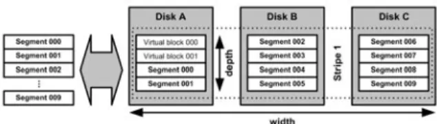
In the particular case of data server clusters, it is of the utmost importance that input/output (I/O) operations be optimized. Techniques such as wide striping[4-6] enable parallel access to an object whose data blocks are distributed over several processors. This technique is illustrated in Fig. 1.
Fig. 1: Wide striping principle
The main goals of a parallel system composed of an architecture and management algorithms are to offer performance, scalability, high processing throughput and high service availability at low cost. In telecommunications, the goal is to reach 7x9s service availability which amounts to about 30 seconds of service interruption per year[7]. Unplanned service interruptions are a consequence of failures caused by hardware, operating system, applications, from errors caused by data access, backup or human manipulations, or from climatic disasters or terrorist attacks, among others[8-10]. The first step in the design of a high availability system (HAS) is to provide a reliable environment. The system must detect and diagnose errors rapidly and apply corrective procedures intelligently. Such an environment can reach up to 3x9s service availability, that is, less than 30 h of service
interruption per year[10]. The critical step in failure recovery is the failover mechanism which redistributes the workload of the failed processor over other processors in the cluster. To be effective, this mechanism needs to be transparent and automatic. In other words, it must not require human intervention. Computer clusters lend themselves particularly well to the concept of failover because of their intrinsically redundant architecture.
A redundancy scheme (RS) is defined by the type of redundancy it provides the system, which can be either data or hardware and by the redundancy management algorithms it implements. Adding a redundancy scheme to a cluster introduce an overhead to query management and processing. The literature offers a wealth of redundancy techniques but as the same time, analysis of these techniques rarely show how they affect quantitatively the cluster’s performance. Furthermore, to our knowledge, there are no quantitative studies on the effect of redundancy schemes on system availability.
This paper evaluates the availability and performance of clusters in terms of redundancy schemes’ properties. More specifically, we designed a cluster model that enables us to analyze a cluster’s behavior in the case of failure of one or several of its nodes. We also propose a general redundancy scheme that can achieve high availability standards.
Background and related work: Here, we present
concepts and techniques pertaining to the implementation of redundancy schemes. Also, we introduce several redundancy schemes that will be used in the solution proposed below.
Hardware redundancy: Failover is a failure recovery
mechanism that exploits hardware redundancy by redistributing the failed node’s workload over other active nodes in the cluster. There are some methods as : N-ways failover and N+m failover.
Fig. 2: N-ways failover
N-ways failover: In N-ways failover, the computer
cluster is composed of N processing units (PU) working jointly and processing incoming transactions. This kind of cluster configuration is called Active/Active since every node in the cluster and its backup are active
during the servicing period[2,10]. All N nodes are primary (active) nodes and backup nodes at the same time. Hence, every node in the cluster has potentially
N-1 backup nodes as illustrated in Fig. 2.
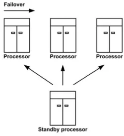
N+m failover: For a cluster composed of N processing
units, there are m backup nodes where each active node is associated one or more backup nodes as illustrated in Fig. 3. In this configuration, also called Active/Standby, backup nodes are in a standby or passive mode[2,10,11]. When a node failure is detected, one or several of its backup nodes are activated and take over its workload. Furthermore, if there are as much active nodes as backup ones where m = N, the model becomes 2xN failover.
Fig. 3: Failover in an active/standby configuration
Data redundancy: The simplest solution to recover
lost data following a disaster or a failure is using backup copies. Two well-known data backup methods are total backup and incremental backup[12]. In the first case, the whole data object is replicated while in the second case, only data blocks modified since the last backup or newly created ones are updated in the backup object. Moreover, updates can be synchronous, meaning they are triggered at regular time intervals or asynchronous which means they are triggered when an object is modified or created.
File objects are sometimes distributed as data blocks like in the wide striping technique. In that case, files are linked to more than one physical memory space. Thus, backup techniques make a distinction between physical memory updates and file or data block updates. Furthermore, to maintain an acceptable throughput, all backups are performed in real-time or while the system is online.
Backup copies must be located somewhere geographically distant from the backup site to prevent loss of the copies during disaster. To facilitate such failure or disaster recovery, restoration scripts for the system and replicated data should be available.
Data replication and chained desclustering: Data
replication simply consists of replicating the desired
data object on one or more distinct processing units[12]. One way to distribute replicated copies over the cluster, also called declustering, is chained declustering[6]. Using this technique, if the primary copy of the object is on processor i, the replicated copies of the object can be distributed on processors j as follows:
]
))[
(
(
i
C
R
N
j
=
+
(1)Where, C(R) is a function that determines the location of the rth replicated object with r=1, 2, 3, …, R,
R is the number of replicated objects and [N] is an
expression meaning modulo and N being the number of processors in the cluster.
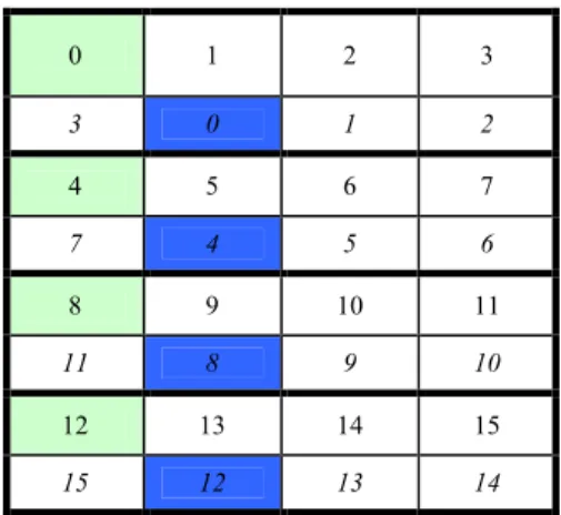
In the simplest form of chained declustering, we have a single replicated object with R = 1 and a distribution function C(R) = 1 which indicates that the replicated object is located on the PU next to the processor where the original copy was located and so on. Figure 4 illustrates the data layout for the aforementioned case. 0 1 2 3 3 0 1 2 4 5 6 7 7 4 5 6 8 9 10 11 11 8 9 10 12 13 14 15 15 12 13 14
Fig. 4: Data layout of the replicated objects
When the cluster detects that processor i has failed, the responsibility fraction (the fraction of queries requiring access to a particular object) of a primary data block and a replicated data object for an active processor j, noted
f
( j
i
,
)
andr
( j
i
,
)
respectively, are given by formulas (2) and (3)[6]:11)}[ ] ( { ) , (i j = N − iN−−j+ N f (2) 1 ] )}[ 1 ( { ) , ( − + − − = N N i j N j i r (3)
Parity, an ECC type scheme: ECC-like (error checking and correcting) schemes are based on computing methods that add several extra bits to the
original data set. These additional bits are used in failure situations, when some part of the data has been lost, to restore the original data. Hence, with this technique, the replicated data set is divided in two parts: the original data set and the parity bits set. Most of the techniques in this family use the exclusive-or (XOR) operation to determine the exact number and type of parity bits that need to be added to the data set.
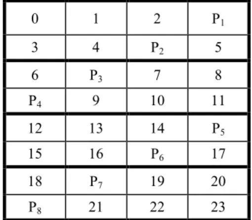
In the computing industry, this scheme is also known as level 3 RAID (Redundant Array of Independent Disks), in which all parity bits are dispersed horizontally over an array of hard drives at the bit level[4,13,14]. Level 4 RAID offers approximately
the same functionality as level 3, but bits, this time, are dispersed by data blocks. Figure 5 illustrates one possible data layout for this scheme, where Pi is the parity block for stripe i.
Data access to an object requires reading one or several of the N-1 processing units holding the desired data. When a transaction modifies the contents of a block, a read/write operation is performed on both the data block and the associated parity block. The latter is updated using an XOR operation.
When one of the cluster’s processing units fails, the original data set can be restored by applying the XOR operation on the data blocks of the remaining PUs, including the parity processing unit. This operation is performed for each stripe. If the failure occurs on the processing unit holding the parity data, it can be restored at a later time while the useful data still being accessible to the users.
0 1 2 P1 3 4 5 P2 6 7 8 P3 9 10 11 P4 12 13 14 P5 15 16 17 P6 18 19 20 P7 21 22 23 P8
Fig. 5: Example data layout for the parity scheme
Cluster reliability: A processing unit is considered to be in failure mode when it exhibits an abnormal behavior, in such a way that the results returned by the PU cannot be used either by the remaining PUs or by the users of the cluster[15-17]. The time between the
detection of the error, leading to a failure and its first occurrence is called the error detection delay. Error detection can be accomplished using different techniques such as self-testing, consisting of the periodical execution by PUs of state validation
programs, or with watchdog timers which are based on query execution time traces and are triggered when the processing time exceeds a certain threshold for the same query[2].
Metrics and reliability evaluation of a cluster:
Among all the failure models available in the literature, we chose to base our analysis on the tolerance-requirements model[18]. This model considers that even
if the system can still process incoming query, it is in failure if it cannot satisfy requirements. Hence, a cluster is in failure if K of its N processing units are in failure, with K < N.
The event causing the failure of a PU follows a random variable for which transitions from one state to another are irreversible. Transition between states is memory-less, in other words, it does not depend on past states and to go back to a preceding state, a restoration process needs to be performed. Furthermore, we consider that the average failure occurrence and variance are constant. The Poisson distribution is appropriate to model this phenomenon[18,19]. Let X be
the random variable for the number of failures of a processing unit, if we know that we have on average loss of service per time unit, then the probability to have n failures in a time interval of t is given by:
[
]
( )
!PrX=n=e t−λnλt n, n=0, 1, 2,… , t >0 (4)
Components and systems availability: In the case of repairable systems, we have to take into account the notion of availability. In a repairable system, all failed components can be substituted with inactive (standby) components and failed components can be reintroduced within the system once they are repaired. The most common definitions for availability include instantaneous availability, noted a(t), availability on a time interval T, noted
a
and the availability taken a the limit when time reaches infinity, also called asymptotic availability and noted A. These last two definitions of availability are given by (5) and (6), respectively:= Ta t dt T a 1 0 () (5)
( )
t a t A lim ∞ → = (6)When a component cannot be repaired its availability strictly corresponds to its reliability. The instantaneous availability of such a component, characterized by an average failures rate λ, can be calculated using formula (7)[18]:
( )
t e ( )t a λ µµ
λ
λ
µ
λ
µ
− + + + + = (7)Where,
µ
=
τ
1
and τ is the average time required to repair the component, or MTTR (mean time to repair). The asymptotic availability can then be calculated with formula (8): MTTR MTBF MTBF A + = + = µ λµ (8)Where, MTBF (Mean Time Between Failures) is the average time between failures and corresponds to
λ1.
Markov chains are an important tool in evaluating the availability of multiple components systems.
For the general case where there are n discrete states, we introduce
Pr
i(t
)
, which means that the system is in state i at time t. The state of the system is calculated using formula (9), while equation (10) shows that the system can only be in one and only one state at time t:Pr
t
Pr
i(
)
=
(9) ==
n i 1Pr
it
1
)
(
(10)ρ
ij
is the transition rate from state i to state j, where i,j=1, 2, 3, …, n, that form the transition matrix P. It has been shown[18] that, under certain conditionsfor P and by resolving the equation
π
P
=
0
, we can obtain the probabilities π, a vector of size n, of finding the system in a given state i at given time t. Another way of finding a solution to the problem is resolving the Chapman-Kolmogoroff equations,π
Q
=
0
, with the constraint that the sum of allπ
ibe equal to 1. Q is the rate transition matrix derived from the transition matrix P.THE PROPOSED REDUNDANCY MODEL
Now, we present our model and formalize some of the concepts introduced earlier. Furthermore, these concepts will be used for analyzing the cluster’s behavior under different failure scenarios.
Modeling the cluster: The cluster model used for this paper is based on the TelOrb model[20,21] and is
composed of several processing units interconnected through reliable 100 Base-T Ethernet switches. A front-end node serves as an access point to the system and as a proxy to the public network. This node accepts incoming queries and distributes them to available PUs.
Moreover, the front-end node is equipped with a memory used to store past cluster states (checkpointing) and for loading applications on processing units when the PUs are booted for the first time or rebooted after maintenance or after a fault occurred.
The cluster plays the role of a server in a mobile communication network and contains user information. Queries addressed to the system can only trigger processes that consult or update user information. We will only consider faults or errors that result in permanent failure of a processing unit. Furthermore, because it is especially difficult to model, failure detection will not be taken into account. Hence, we consider that the failure detection system in place is reliable and each failure is detected and located, covering 100% of the cluster. These constraints do not hinder the evaluation of the cluster’s availability since the average time taken to detect a failure is negligible when compared to the average time required to repair the failure.
In short, the cluster under consideration is a system for which read/write queries are fairly distributed over a finite set of identical processing units (P1, P2, … , Pn) that share a single network space and equipped with a distributed database utilizing the wide striping technique for data redundancy.
Failover in the Active/Active configuration: In this configuration, all N processing units are both primary (active) nodes and backup nodes for each other. Hence, every node in the cluster has N-1 backup nodes. The fact that all processing units are active at the same time allows the cluster to carry out “hot” failover, also called hot swapping. In this particular case, failover is completed faster than when one or several standby or inactive nodes have to be awaken before redistributing the failed node’s workload. However, since all processing units are active at the same time, they all are subject to a failure rate λ. As a consequence, the failure rate is N×λ for a cluster of N PUs. Under normal operation (no failures), the cluster’s performance is greater than in the Active/Standby configuration since all N PUs process incoming queries which in turn increases the processing throughput of the cluster as a whole. Nonetheless, as we have already mentioned, this increase in performance is not free since the overall risk of a failure occurring on one or more PUs is also greater. Under failure operation, this configuration performs better than its counterpart mostly because failover time is reduced to its minimum and thus might also improve the overall system’s availability.
Let’s consider a cluster designed to process R queries per second with N processing units and with an average response time T. If the cluster looses one processing unit while the N-1 remaining PUs function at full capacity, then the cluster’s overall performance might degrade noticeably, especially if the failover occurs from one PU to another instead of one PU to N-1
PUs. Indeed, the distribution of the failed node’s transactions over N-1 PUs reduces the rate variation of incoming queries and thus stabilizes each PU’s workload.
Failover in the Active/Standby configuration: It is possible to design a cluster with N+m processors where m passive nodes are used as backup nodes for the N active nodes. The challenge with this configuration is choosing the value of m in such a way that it increases the availability of the system without substantially increasing the overall cost of the cluster. It is important to note that the cluster’s original cost increases by a factor proportional to +
N m
1 when this configuration is used.
Failover delays in the Active/Standby configuration are greater than in the Active/Active configuration because the backup node must go through a transition phase not required in the latter. This kind of failover can also be called warm failover in opposition to the hot failover where the transition phase is almost instantaneous. Thus, if a hot failover requires a delay d to complete, then a warm failover will require a delay of (2-3d) to complete[22-25].
When analyzing this scheme under the angle of availability, we have to consider three characteristics or rates: the average failure rate (N×λ), the average repair time rate ( r) and the average failover rate ( s). A state is then characterized by the number of processing units under reparation and the number of available or active PUs. Since the failover and repair time rates are much greater than the failure rate, we can limit the analysis of the present scheme to states containing two simultaneous failures without dramatically changing the ensuing results. Hence, if we consider this simplified analysis model, we obtain a triangular Markov system.
In the case where m equals N, the cluster is composed of 2×N processors. Hence, the cost of the cluster is twice as much as the cost of the original cluster. This new configuration possesses two advantages over the N×m configuration. First, it offers the possibility to implement a decentralized control, which means that no particular node has to perform failure detection and second, it is possible to mimic the hot swap or hot failover technique as with the Active/Active configuration[10,26].
Disaster recovery: The aforementioned schemes cannot prevent every type of system failure. Indeed, in the event of a physical disaster like an earthquake, a fire, or a failure of the SS7 link linking the cluster to the network, for example, a redundancy scheme alone may not be suitable and thus to restore the system to the state it was in before the disaster occurred a recovery scheme is needed. The 2×N scheme mentioned in the presentation of the Active/Standby configuration, in spite of its high cost, may be beneficial in such a
scenario in the sense that the N primary and N backup nodes may be geographically distant from one another while being connected through a TCP/IP WAN (Wide Area Network). The difficulty here is to maintain coherence between the databases of the two sites. To improve performance, it is of good practice to adopt an optimistic approach and thus, to do regular non-blocking transaction updates from site to site but also to validate regularly (at regular time intervals or after a given number of replications) the coherence of the data between the two sites. In an Active/Active configuration, each site manages half of the cluster’s traffic and hence half of the data. One advantage of this configuration is that it offers better transaction throughput than its counterpart since transaction replication requires less resources than transaction creation[21]. It is worth noting that only transactions
modifying at least one traffic object are replicated. Each processing unit runs the software processes required for asynchronous, incremental and online replication of transactions modifying traffic objects. Furthermore, PUs are also equipped with independent TCP/IP connections linking them to their backup node and used to deliver IP packets in a reliable way. However, since TCP/IP does not preserve packet order, it is possible that transactions may not be recorded in their execution order. In other words, a newer transaction may be recorded at the backup site before an older one. A simple solution to this problem is to allocate IDs to transactions in order to preserve their execution order and markers to created or deleted objects.
Data redundancy: We consider that replicated objects are updated incrementally and that only records modified by a transaction are updated. In fact, only transactions concerning primary objects are copied and applied to the replicated objects. Updating is performed asynchronously since in a mobile communication network modifications happen frequently. For replication schemes that take into account file continuity, like in wide striping, file restoration can be performed relatively fast in case of system or component failure. However, file backup operations are slowed down because they require additional operations to search for the adequate data blocks and result in an overload of memory accesses and hence in a decrease of data throughput. On the other hand, a replication scheme based on the physical location of data blocks increases backup performance while it complicates and slows down file restoration. Moreover, no asynchronous updates are possible with this scheme.
Replication scheme: The main drawback with this scheme is the need to double the total memory capacity of the cluster. In normal operational mode (no failures), the read operation is performed on the two copies (original and replicated), which should improve performances when reading data. While performing a
read operation, the system is required to validate every transaction on the original data as well as on the replicated data. The exact number of replicated object depends on the type of applications used, on access frequency and on the probability to loose a PU. It is possible to approximate the probability to loose data when the object is replicated at the memory space level and not at memory blocks level, which means that every replicated object on processor a is replicated on processor b. If we limit the size of the Markov chain to a maximum of 4 states (this allows a maximum of two failures in a given time period) and considering a cluster of size N=8 with a failure rate of λ=500 h and a replacement or repair time rate of µ=5 h, we get a probability equal to 0.0008 of loosing data, which amounts to about 7 h of downtime per year.
When the cluster is in failure mode, queries intended for processor a are rerouted towards processor b which in turn, implies that the latter processor’s workload is increased while its performance decreases, especially if processor b’s initial workload was over 50% of its capacity. In such situation, the overall performance of the cluster decreases since the initially uniformly distributed workload is now more or less randomly distributed over the available processors. Thus, to efficiently redistribute queries to all processors we have to decluster data on a per block basis. In this case, we have C(R) = k [N], with k = 0 initially and incremented one unit each time we have determine the next location of the replicated block. An example data layout obtained from this scheme is illustrated in Fig. 6. If we consider that each block is accessed with the same frequency, each available processor’s overload increases uniformly when one processor in the cluster fails. Although, it improves overall performance, the probability to loose data blocks increases up to 0.0745 which approximately equals 27 days of downtime per year. A solution to reduce this downtime is to create relative clusters which are mini-clusters composed of m of the N original processors. Thus, we now have
m
N
M =
relative clusters for which declustering can be performed independently. If we consider the aforementioned constraints and divide the original cluster in two relative clusters of 4 processors each, it is possible to reduce the cluster’s overall downtime to 19 h per year.Parity, an ECC type scheme: This scheme induces an increase in memory requirements proportional to
N1 . At first, we note that it does not seem suitable for applications in which data is frequently modified. Indeed, to restore lost data, the scheme requires an intensive access to the Nth processor that holds the parity blocks. This in turn overloads the parity processor, which becomes the bottleneck of the cluster
0 1 2 3 3 0 1 2 4 5 6 7 7 4 5 6 8 9 10 11 11 8 9 10 12 13 14 15 15 12 13 14
Fig. 6: Data layout for the multiply chained declustering scheme 0 1 2 P1 3 4 P2 5 6 P3 7 8 P4 9 10 11 12 13 14 P5 15 16 P6 17 18 P7 19 20 P8 21 22 23
Fig. 7: Data layout for parity blocks distributed over all processors
and limits its performances. To enhance the performance of the cluster in failure mode operation, one solution is to initially distribute parity blocks over all processors, as illustrated in Fig. 7.
In this configuration, all nodes hold both data and parity blocks. The configuration only permits failure of a single processor at a given time. We can improve this by creating several relative or mini-clusters that form disjoint parity sets. The new configuration, as illustrated in Fig. 8, can tolerate the loss of a processor in each mini-cluster and thus increases the overall tolerance of the cluster. If we divide the N processors of the cluster in groups of m processors, with m N, we now have
m N
M = mini-clusters and the cluster as a
whole could tolerate up to M failures at the condition they happen in M distinct groups or mini-clusters. To give an idea of the improvement, we consider that the failure of a processor follows an exponential law with parameter λ = 500 h, that the time required to repair or replace a processor is given by µ = 5 h and that there are 8 processors divided in two mini-clusters of 4
processors each. The probability to have two processors failing at the same time, one in each group, is 0.0745 while the probability of having two processors failing in the same group is 0.0022. The probability to loose data, or in other words to have three processors failing at the same time, is 0.0003, which amounts to 2.5 h of downtime per year. Moreover, if we include an N+m failover scheme, we can further reduce the downtime. 0 1 P1 2 3 P9 4 P2 5 6 P10 7 P3 8 9 P11 10 11 12 13 P4 14 15 P12 16 P5 17 18 P13 19 P6 20 21 P14 22 23 24 25 P7 26 27 P15 28 P8 29 30 P16 31
Fig. 8: Data layout of the parity scheme on two relative clusters
ANALYTICAL AND SIMULATION RESULTS
Now, we presents the results for the availability of the cluster. These results where obtained from two phases of simulation. The first phase implements a simple model that will enable us to validate analytical results while the second phase implements a more realistic model allowing more precision in the results.
Availability of the cluster: Analytical results
N-ways scheme processor availability: In the case of
the N-ways failover scheme, the solution to the problem of maximum availability can be reduced to resolving an irreducible Markov chain consisting of a birth and death process whose states are characterized by the number of failed processors. An example of such a Markov chain is given in Fig. 9. The failure or repair time rate of a processor marks the transition between states.
Fig. 9: Analytical model of the N-ways scheme This model is equivalent to an M/M/1/N/N queue, using Kendall’s notation, where N is the number of processors in the cluster. The model is also known in the literature as the machine-repair model[27]. The
probability to find k processors failing at the same time in the cluster can be calculated with formula (11):
= − − = N j N j k N k k j 0( 1 )! )! ( ρ ρ π (11)
We consider that the system is unavailable after one of its processor fails, hence we have:
0
π
=
A
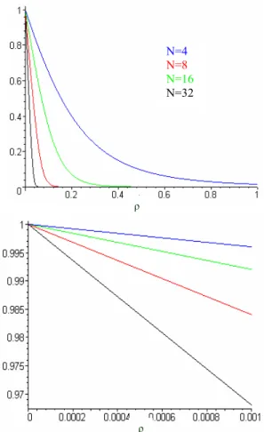
(12)Figure 10 illustrates the availability of the cluster as a function of
µ λ
ρ= and for different number of
processors N in the cluster (4, 8, 16 and 32). We note that there is a high availability value (99%) when is in the order of the thousandth. When increases, the availability of the cluster drops sharply. The degree at which the availability drops depends on the number of processors in the cluster. Thus, to maximize the cluster’s availability, we have to minimize the value of as well as the number of processors. So, to obtain cluster availability in the neighborhood of 99.9%, we need a value of less than or equal to 0.0001. In other words, the mean time to repair (MTTR) needs to be about 10000 times inferior to the mean time between failures (MTBF).
Fig. 10: Availability results for N=4, 8, 16 and 32 processors as a function of
N+m scheme processor availability: If we consider that in general is in the order 0.00002 at a minimum[28], then the only logical way to achieve 7x9s
is by applying the N+m scheme to the cluster. The most precise model describing this scheme consists of a closed network of three queues as illustrated in Fig. 11.
Fig. 11: Closed network model with three distinct queues of the N+m scheme
The fist queue represents active processors or, in other words, processors waiting to service incoming queries. In Kendall’s notation, the queue would be noted as M/M/N/N, where the first N is the number of servers while the second N represents the number of queries the system can process. It is worth noting that the number of queries the system can process at one time exactly matches the number of processors within the system. Hence, we have at most one query per processor. Service time corresponds to the time between failures and is equal to
λ1. The second queue represents a processor’s repair process and is modeled with an M/M/1 queue with a service rate of µ. Finally, the third queue models a processor waiting to take over a failing processor. The queue used here is M/M/ where the average service rate equals the average delay required to complete a failover.
All in all, we have a network where the first queue has fixed capacity while the other two have infinite capacity. Hence, we can say that the model creates a non-homogenous network. Moreover, we have a blocking system since, for example, a processor cannot be processed on queue 3 before a server on queue 1 is free. This type of blocking action is called blocking before start (BBS)[19,29]. The number of queries L in the
system equals the number of active processors to which we add all waiting processors so that L=N+m. We will now reduce this network so as to obtain an analytical solution.
We consider that the delay induced by the failover is negligible and is equivalent to passing a query from the queue to the server. This simplification results in a closed network with two queues, where queue 1 becomes an M/M/N queue with unlimited capacity while queue 2 stays the same. By resolving the system (the details are given in appendix A), we get the following expression: j N N L j G N A= −
N
= µ λ ! 0 (13) N=4 N=8 N=16 N=32where:
(
)
1 1 1 1 1 ! ! − + − + − = − − + − = L ρ N ρLρN N L n n n L N N n L N N G (14)The traces In Fig. 12 show availability results obtained for a cluster composed of 4, 8, 16 and 32 processors and a processor waiting for service (L=N+1).
Fig. 12: Availability results for an N+1 model
The four curves can be differentiated by the speed at which availability drops as the value of increases. Furthermore, we note that the range of values for which availability is high augments as the value for L increases from N. In this way, it is possible to achieve 7x9s availability with a reasonable value for (for L=N+2, ’s value is in the order of 0.005 which corresponds to an average repair time 200 times superior to the time between failures). To adequately compare this scheme with N-ways, we suppose that both schemes’ costs are equal and that they each use L processors. The cluster is available as long as there are N processors to service incoming queries. Simulation results obtained for both schemes are based on the assumption that the average failure rate for processors in waiting state is null. The behavior of the N+m and N-ways schemes for L=N+2 is depicted In Fig. 13.
As we have seen in a precedent section, we can have an N+m configuration for which L=2×N. It is obvious that in that case, as Fig. 14 shows for a cluster of N = 4 processors, the cluster’s availability is greater than in any of the configuration seen so far. Indeed, we observe that the minimal availability is about 72% while the 7x9s availability can be achieved with relatively high values of ρ. On the down side, this configuration is costly when compared with the other two and is not profitable unless we have a suitable value for (in the neighborhood of 0.2). It is important to mention that the results just presented are valid if partial failover (a failed processor in the first site is relieved by its backup in the backup site) is allowed between the two sites.
Fig. 13: Availability comparisons of the N+m and N-ways for L=N+2
Fig. 14: Availability results for the 2×N configuration with N = 4
Data availability: We analyze different data protection configurations in order to better understand their influence on the cluster’s availability in terms of data accessibility and we determine to what measure the loss of a processor can induce loss of data. When no redundancy schemes are applied, the loss of a processor automatically induces loss of data. If we assume that when data is lost the cluster becomes unavailable, then in this context the cluster’s availability can be calculated using equation (9).
There are many alternatives or models to choose when applying a replication scheme. Two parameters common to all replication schemes are the number r of replicated objects and the relation established between the processors holding primary data and those holding backup or replicated data. Since the main drawback of all replication schemes revolves around memory size, we limit our analysis to schemes generating a single replicate. These alternatives are distinguished by the relation they create between primary and replicated data. The first replication scheme we introduce is based on a static relation that assigns a backup processor j to N=4 N=8 N=16 N=32 N=4 N=8 N=16 N=32
each primary processor I and inversely. The second alternative or model assigns backup processors in chain following j=i+1 [N], where j is a backup processor, i a primary processor and N the number of processors in the cluster. The third considered model follows equation j=i+k [N] where k is incremented for each data block and hence, replication is done on a per block basis. The principal advantage of this last model is that, when in failure mode operation, queries addressed to lost processor i are rerouted towards all remaining processors, uniformly redistributing the lost processor’s workload and preserving the cluster’s performance.
If we assume that at a given time the cluster operates with n < N, there are p lost processors (p = N - n). The probability to find the cluster in such a state is given by Sp. To determine the cluster’s availability, we have to evaluate, for each model presented, the probability of having all data available, noted Sp. As for the parity scheme, the probability of having unavailable data following the failure of p processors is closely related to the number of mini-clusters in use. Indeed, when at least two processors within the same mini-cluster have failed, data becomes automatically unavailable. Thus, by resolving the different data redundancy models using results detailed in Appendix B, we find that the cluster’s availability D can be expressed by: = = + + + = /2 2 1 0 ( ) () ( ) N j j Rj m P jRj m D (15)
Where, P depends on the redundancy scheme applied to the cluster (parameterized replication or parity). The variable parameters that we have to watch for are N, L and for all replication schemes and M for the parity redundancy scheme.
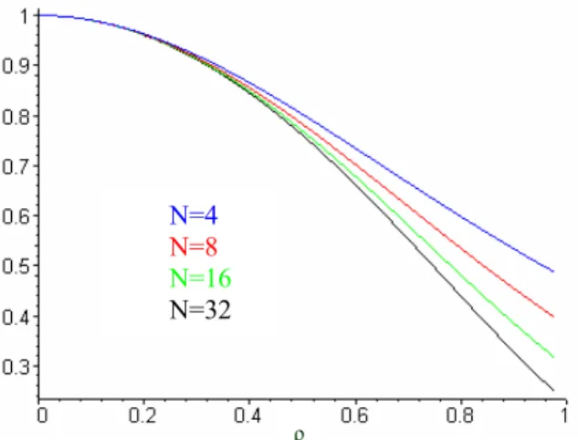
Figure 15 and 16 show data availability for a cluster composed of 8 and 16 processors, respectively, for two replication schemes and several parameters for the parity scheme. As we can see, the first replication model (model 1) offers the highest cluster availability. Moreover, its availability does not become null when ρ reaches its limit of 1. The cluster’s availability when we apply the parity scheme with 2 mini-clusters is the lowest of all simulated schemes and its performance is equivalent to the second replication model (model 2). On the other hand, when we apply the same parity scheme with 4 mini-clusters, the resulting availability curve closely follows the first replication scheme’s curve and offers better performance when compared to the second replication scheme.
It is important to note that, when the number of processors is sufficiently high, all schemes offer approximately the same availability level, whatever the number of mini-clusters in the parity scheme. In fact, the number of processors per mini-cluster is more important than the number of mini-clusters itself.
Fig. 15: Data availability results for a cluster composed of 8 processors
Fig. 16: Data availability results for a cluster composed of 16 processors
Finally, we observe that the curves tend to move away from one another as the value of increases.
Performance analysis: To analyze the impact on the cluster’s performance of the schemes presented so far, we developed a second simulator. This simulator is based on the cluster model presented earlier. We calibrated the simulator so that the range of incoming queries would be limited at a maximum to 4000 queries per second. The first results obtained from the simulator give the average response time for a cluster operating without any redundancy scheme. These results are in the order of the millisecond (as TelOrb’s traffic manager) and will serve as a reference for comparison with clusters running a replication or parity scheme. The first step of the simulation is to determine the average value of the schemes’ parameters and to evaluate these schemes so as to choose one in each class based on its relative performance to the baseline. Afterwards, we analyze the impact of the schemes’ parameters on the cluster’s performance with the aforementioned three schemes.
We start by analyzing the impact of update operations, given in percentage, on the cluster’s
+++ Model 1 (replication) Model 2 (replication) Parity 1 (M=2) Parity 2 (M=4) +++ Model 1 (replication) . . . Model 1 (replication) Parity 2 (M=4) Parity 3 (M=8)
0 200 400 600 800 1000 1200 0 100 200 300 400 500 600 réplication parité référence Write/total 10%
Queries/10 per second
Thr ou ghpu t /10 per se con d Replication Parity Reference 0 200 400 600 800 1000 1200 0 100 200 300 400 500 600 réplication parité référence Write/total 10%
Queries/10 per second
Thr ou ghpu t /10 per se con d Replication Parity Reference 0 200 400 600 800 1000 1200 0 50 100 150 200 250 300 350 400 450 500 réplication parité référence Write/total 20%
Queries/10 per second
Th ro ug hp ut /1 0 p er se con d Replication Parity Reference 0 200 400 600 800 1000 1200 0 50 100 150 200 250 300 350 400 450 500 réplication parité référence Write/total 20%
Queries/10 per second
Th ro ug hp ut /1 0 p er se con d Replication Parity Reference 0 200 400 600 800 1000 1200 0 50 100 150 200 250 300 350 400 450 500 réplication parité référence 8 processors
Queries/10 per second
Thr ou gh put /1 0 pe r se co nd Replication Parity Reference 0 200 400 600 800 1000 1200 0 50 100 150 200 250 300 350 400 450 500 réplication parité référence 8 processors
Queries/10 per second
Thr ou gh put /1 0 pe r se co nd Replication Parity Reference 0 200 400 600 800 1000 1200 0 100 200 300 400 500 600 réplication parité référence 32 processors
Queries/10 per second
Th ro ug hp ut / 10 pe r s ec on d Replication Parity Reference 0 200 400 600 800 1000 1200 0 100 200 300 400 500 600 réplication parité référence 32 processors
Queries/10 per second
Th ro ug hp ut / 10 pe r s ec on d Replication Parity Reference
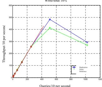
throughput. To do so, we fix the number of nodes in the cluster to 24 and vary the update percentage from 10 to 20%. The ensuing results are scaled by 10 so we can better observe the differences between the curves. Figure 17 (a) and (b) show the cluster’s throughput for update percentages of 10 and 20%, respectively.
a) Cluster throughput in percentage: 10%
b) Cluster throughput in percentage: 20% Fig. 17: Cluster throughput in percentage
As we can see, the curves follow similar trends. We note that when the cluster enters its critical zone (its maximum value for the query rate), the curves show substantial differences in terms of throughput. Moreover, we observe that the curves start moving apart from one another when the incoming query rate reaches 2500 queries per second, then the curves’ slope decreases dramatically. The impact on the parity scheme’s throughput is more important than for the replication scheme. The difference in results for the two schemes increases as the percentage itself increases. Such discrepancies can be explained by the fact that additional memory accesses are required by the parity
scheme. Finally we will analyze, for the two chosen schemes, the impact of the number of nodes on the cluster’s behavior. To do so, we fix the update percentage to 10% and vary the number of node in the cluster from 8 to 32 nodes. Figure 18 (a) and (b) illustrate simulation results obtained for these two scenarios. We observe that, as we increase the number of nodes in the cluster, the curves move apart from one another. Indeed, we note that the parity scheme’s throughput moves away from the reference while the replication scheme’s throughput closes on the baseline throughput.
a) Cluster throughput for 8 processors
b) Cluster throughput for 32 processors
Fig. 18: Cluster throughput for different number of processors
CONCLUSION
In this study, we have proposed some redundancy schemes to insure availability and quality of service of computer clusters. The main goal as to maximize a
cluster’s availability, by applying several redundancy schemes while minimizing their impact on overall system performance. In this context, two important properties of the system are the cluster’s throughput (number of queries processed by unit time) and its response time (time required to service a query).
We found that two important aspects influencing the performance of a transaction-oriented cluster were the cluster’s failover and data redundancy schemes. The resulting schemes were analyzed in two phases. In the first phase, we simulated an analytical model in order to better understand the impact of these schemes’ implementation parameters on the cluster’s availability. We observed that the N+m failover scheme with a standby processor offered higher availability than the N-ways scheme for values of in the range of the thousandth. We were able to attain 5x9s availability with this scheme. Moreover, when m = N, we observed that the minimum availability exceeded 72% and that 7x9s availability could be obtained with relatively high values of . We simulated several data redundancy schemes and found that data replication offered higher cluster availability than the parity model. The latter scheme’s performance approaches replication either when we increase the number of mini-clusters or reduce the number of nodes in each mini-cluster. It is interesting to note that when the number of nodes in the cluster is sufficiently high, all schemes offer similar availability notwithstanding the number of mini-clusters for the parity scheme. Also, we observed that the cluster’s throughput increased almost linearly for all schemes in the 0 to 5000 queries per second range. When the number of incoming queries exceeded the rate of 5000 queries per second, we observed that the curves moved apart from one another and that service quality dropped significantly. This phenomenon does not depend on the scheme applied to the cluster but seems related to the cluster’s processing power.
Moreover, our analysis shows that parity with the maximum allowable number of mini-clusters and replication with an incrementable backup processor index offer the best performances in each scheme’s class. The difference between those two schemes, with a slight advantage for replication, increases as the percentage of update operations increases. In the same way, as the number of cluster nodes increases the difference in performance between the two schemes becomes more visible. A better comparison would require comparing two architectures with equal costs or to compare the cost of two architectures with similar performances. Another way to solve the problem would be to consider that parity, for a given memory size, allows more user data to be stored than replication. Hence, the incoming query rate can be increased by
C
N2+N , which in turn implies a better throughput. For comparison purposes, we would have to apply a translation to the right to the parity curve. The parity
scheme would then have a higher throughput in the zone where the rate is positive while its maximum throughput would still remain inferior to the replication scheme’s and reference model maximum throughputs. This trick is only valid when in the zone where the rate is positive since, when the rate is negative, the parity scheme’s throughput would be penalized. In other words, it works in a context where the cluster is not limited by its CPU’s performance or by memory accesses. We came to the conclusion that in practice, this comparison is not necessary since in general the cluster’s acquisition budget is fixed. In these conditions, the methodology used to choose the best fitted redundancy scheme among the ones available is: * To determine the number of nodes (2P) that can be
acquired with the allocated budget
* We can choose one of the following two failover schemes:
* N-ways configuration with 2P nodes * N+m configuration with N+m = 2P
* To identify the right configuration to implement, we have to determine the cluster’s performance threshold in terms of throughput or response time, which will allow us to define the exact number of active processors (PA)
* The PA parameter is determined by analyzing the comparative performance in terms of incoming query rate, which depends on the number of clients, for the parity and replication schemes under normal and failure operation mode
* We can now choose the most appropriate data redundancy scheme according to desired cluster performances. If the replication scheme is chosen, we have to assert that PA < P+1 at all times
* Finally, if PA < 2P, we can apply the N+m scheme with m = 2P - PA. If this condition does not hold, we can always choose an N-ways scheme.
It would be advantageous to analyze the cluster’s behavior in the case of large size read/write operations. Indeed, in our context, we considered that user data corresponded to a mobile telephony client’s data and was about 8 Kb in size. If we apply wide striping to the PVFS file system, for example, default data blocks are about 64 Kb in size which implies that access to an object is equivalent to an access to a single cluster node. For applications such as video on demand (VoD), the average data size of a query would in the order of megabits.
Appendix A: This network possesses a stationary state and the solution is given as a product:
∏ = = 2 1 ( ) ) ( i f isi G s R (1)
Where, s is a state vector representing the number of processors in the system (a queue and its servers form a system). The contribution of queue i is given
by
f
i
(si
)
while G is a normalization constant, necessary because it’s a closed network and the number of processors is constant as well. According to BCMP[19,29,30], the probability R(s) to be in a given states = (s1, s2) can be calculated based on formula (2):
)
(
)
(
)
(
s
G
f
1s
1f
2s
2R =
(2) with < = otherwise. , 1 ! if , 1 ! ) ( 1 1 1 1 1 1 1 s N s s N N N s s N s f λ λ (3) and s s f2( 2)=µ
1 2 (4)knowing that each query goes through both queues which means that the visit ratio for each queue is equal to 1. So if we substitute (3) and (4) in (2), we get:
< = otherwise. , 1 1 ! if , 1 1 ! ) ( 2 1 2 1 1 1 1 s s N s s s N N G N s s N G s R µ λ µ λ (5)
Since we know that the system is a closed network, we have L = s1 + s2 at all times. Hence, we can eliminate a variable by substituting s1 = L - s2 in equation (5) and get a single variable equation given by equation (6): − − ≤ = otherwise. , )! ( if , ! ) ( 1 j L j s N j L N G N L j N N G s R µ λ µ λ (6)
To define the constant G, we know that the sum of probabilities for all L processors in the system must equal 1 and thus, we get:
(
)
1 1 1 1 1 ! ! − + − + − = − − + − = L ρ N ρLρN N L n n n L N N n L N N G (7)Now that we have the probability of having j processors in the repair queue at the same time, we can determine the cluster’s availability. Indeed, we consider that the system is available as long as we have N active (in service) processors, or in other words, as long as there less than L-N in the repair queue. So, the system’s availability can be calculated using expression (8):
− = =L N j j N N N G A 0 !
µ
λ
(8)Appendix B: If we consider that cluster operates with n < N processors at a given time, there are p failed processors (N = n + p). The probability to find the cluster in that sate is given by Sp. To calculate the cluster’s availability, we first need to determine the probability of having all data available at a given time for the replication and parity schemes, noted Pp. Hence, we have Pp = 1 when p r and Pp = 0 when p >
2 N , which is also valid for the parity scheme. Let’s consider first the relation used for the third replication scheme. In that case, all processors are linked together to improve data protection and thus, the failure of at least two processors automatically implies that data is unavailable. The cluster’s availability in such situation is equivalent to having N-2 or less active processors and can be calculated using formula (1):
=
=
N p pS
D
2 (1) For the first relation it is possible to determine, using equation (2), the probability of not having any one pair of processors linked together among the p > 1 failed processors.( )
! )! 1 2 ( )! (! 2 2 1 N p N p N N p p p + − − = 1< p N2 (2)As for the second replication relation, we cans show that: ) 2 )( 1 ( 2 1 2 = N− N− p p p p 1< p N2 (3)
It is important to note that we consider that we have an even number of processors. We can justify this constraint by the fact that if we need j nodes to service a given number of clients, we will have a total of 2j nodes after applying replication.
As for the parity scheme, the probability of having unavailable data following a failure of p processors closely depends on the number of mini-clusters implemented within the cluster. Indeed, when two or more processors within a single mini-cluster are lost, some of the data becomes unavailable and hence, the cluster’s itself becomes unavailable. So for the parity scheme, we have Pp = 1 when p > M, the number of mini-clusters. In the case where p M, the cluster’s availability (all data is available) can be calculated as follows: )! (! )! (! p M N p N M pp= −− p M (4)
It is worth noting that all mini-clusters must have the same number of processors and thus, N is a multiple of M. These considerations are both practical and mathematical. A well balanced workload over all processors leads to better performance of the cluster.
Since we have now defined data availability probabilities for all schemes, we can determine the cluster’s overall data availability D, which is given by:
P p N p S p D = = 0 (5) When the N-ways scheme is applied, Sp is equal to p
and when an N+m scheme is used, we can define Sp as
the probability of having m+p processors out of service. If we take into account this assumption, we can calculate the cluster’s availability using formula (6):
= = + + + = /2 2 1 0 ( ) () ( ) N j j R j m P jR j m D (6)
Where, P depends on the redundancy scheme applied to the cluster (parameterized replication or parity).
REFERENCES
1. Buyya, R., 1997. Single System Image: Need, Approaches and Supporting HPC Systems. The 1997 Intl. Conf. Parallel and Distributed Processing, Techniques and Applications (PDPTA’97). CSREA Publishers, Las Vegas, USA, pp: 1106-1110.
2. Buyya, R., 1999. High Performance Cluster Computing: Architectures and Systems. Prentice Hall, New Jersey.
3. Pfister, G., 1998. In Search of Clusters. Prentice Hall PTR, NJ, 2nd Edn., N.J.
4. Chen, P. and G. Gibson G., 1990. An Evaluation of Redundant Arrays of Disks Using an Amdhal 5890. Joint Intl. Conf. Measurement and Modeling of Computer Systems, Colorado, pp: 74-85. 5. Gordon, D., 2002. The floating column algorithm
for shaded, parallel display of function surfaces without patches. IEEE Trans. Visualization and Computer Graphics, 8: 76-91.
6. Hsiao, H.I. and D.J. DeWitt, 1990. Chained Declustering: A New Availability Strategy for Multiprocessor Database Machines. Proc. 6th Intl. Conf. Data Engineering, Los Angeles, CA, pp: 456-465.
7. Shen, K., T. Yang and L. Chu, 2003. Clustering support and replication management for scalable network services. IEEE Trans. Parallel and Distributed Systems, 14: 1168-1179.
8. Gray, J., 1986. Why do Computers Stop and What Can be Done About It? 5th Symp. Reliability in Distributed Software and Databse Systems, Los Angeles, CA, USA, pp: 3-12.
9. Siweiorek D.P. and R.S. Swarz, 1983. The Theory and Practice of Reliable System Design. Digital Press, Digital Equipment Corporation.
10. Weygant, P.S., 1996. Clusters for High Availability-A Primer of HP-UX Solutions. Hewlett-Packard Company, Prentice Hall PTR, Upper Saddle River, New Jersey 07458.
11. Copeland, G. and T. Keller, 1989. A Comparison of High-Availability Media Recovery Techniques. Proc. ACM-SIGMOD Intl. Conf. Management of Data, Portland, pp: 98-109.
12. Zou, H. and F. Jahanian, 1999. A Real-Time Primary-Backup Replication Service. IEEE Trans. Parallel and Distributed Systems, 10: 533-548. 13. Alvarez, G., W. Burkhard and C. Flaviu, 1997.
Tolerating Multiple Failures in RAID Architectures with Optimal Storage and Uniform Declustering, 1996. Proc. ACM/IEEE 24th Ann. Intl. Symp. Computer Architectures, Denver, Collorado, pp: 62-72.
14. Sorin, D., M. Martin, M. Hill and D. Wood, 2002. SafetyNet: Improving the availability of shared memory multiprocessors with global checkpoint/recovery. Proc. 29th Ann. Intl. Symp. Computer Architecture, pp: 123-134.
15. Bhargava, A. and B. Bhargava, 1999. Measurements and Quality of Service Issues in Electronic Commerce Software. Proc. 1999 IEEE Symp. Application Specific Systems and Software Engineering & Technology, Richardson, Texas, pp: 26-33.
16. Deris, M., M. Rabiei, A. Noraziah and H. Suzuri, 2003. High service reliability for cluster server systems. IEEE Intl. Conf. Cluster Computing, pp: 280-287.
17. Lopez, M. and S. Wood, 2003. Systems of multiple cluster tools: Configuration, reliability and performance. IEEE Trans. Semiconductor Manufacturing, 16: 170-178.
18. Modarres, M., M. Kaminskiy, V. Krivtsov and M. Dekker, 1998. Reliability Engineering and Risk Analysis: A Practical Guide. New York, N.Y. 19. Balsamo, S. and V. De Nitto Personè, 1991. Closed
Queueing Networks with Finite Capacities: Blocking Types, Product-Form solution and Performance Indices. Performance Evaluation, 12: 85-102.
20. Hennert, L. and A. Larruy, 1999. TelOrb-The Distributed Communications Operating System. Ericsson Review, No. 03.
21. Hennert, L. and A. Larruy, 2000. TelOrb Network Redundancy. Ericsson Review, No .02.
22. Banchini, R. and E.V. Carrera, 2000. Analytical and Experimental Evaluation of Cluster-Based Networks Servers. Technical Report 718, Department of Computer and Sciences, University of Rochester.
23. Chang, W., 2001. A resource efficient scheme for network service recovery in a cluster. IEEE Intl. Conf. Systems, Man and Cybernetics, 2: 1087-1091.
24. Cretu, A., V. Groza, A. Al-Dhaher and R. Abielmona, 2002. Performance evaluation of a software cluster, Proc. 19th IEEE Conf. Instrumentation and Measurement Technology, 2: 1543-1548.
25. Gail, H.R. and E. Souza e Silva, 1992. Performability Analysis of Computer Systems: From Model Specification to solution. Performance Evaluation, 14: 157-196.
26. Yong, C., L. Ni, X. Chengzhong, Y. Mingyao, J. Kusler and Z. Pei, 2002. CoStore: A reliable and highly available storage system using clusters. Proc. 16th Ann. Intl. Symp. High Performance Computing Systems and Applications, pp: 3-11. 27. Molloy, M., 1988. Fundamentals of Performance
Modeling. Macmillan Publishing Company, NY. 28. Carreira, J., H. Madeira and J. Silva, 1998.
Xception: A technique for the experimental evaluation of dependability in modern computers. IEEE Tran. Software Engineering, 24: 125-136. 29. Balsamo, S., V. De Nitto and R. Onvural, 2000.
Analysis of Queueing Networks with Blocking. Kluwer Academic Publishers, Boston, Hardbourg. 30. Balsamo, S., 2000. Closed Queueing Networks
with Finite Capacity Queues: Approximate Analysis. Proc. ESM 2000, SCS, European Simulation Multiconference, Ghent, pp: 23-26.