HAL Id: hal-00618967
https://hal-mines-paristech.archives-ouvertes.fr/hal-00618967
Submitted on 4 Sep 2011HAL is a multi-disciplinary open access
archive for the deposit and dissemination of sci-entific research documents, whether they are pub-lished or not. The documents may come from teaching and research institutions in France or
L’archive ouverte pluridisciplinaire HAL, est destinée au dépôt et à la diffusion de documents scientifiques de niveau recherche, publiés ou non, émanant des établissements d’enseignement et de recherche français ou étrangers, des laboratoires
Variance scaling of Boolean random varieties
Dominique Jeulin
To cite this version:
Variance scaling of Boolean random varieties
Dominique Jeulin
Centre de Morphologie Mathématique Mathématiques et Systèmes
Mines ParisTech
35 rue Saint-Honoré, F77300 Fontainebleau, France email: [email protected],
26-08-2011
Abstract
Long …bers or strati…ed media show very long range correlations. This media can be simulated by models of Boolean random varieties. We study for these models the non standard scaling laws of the variance of the local volume fraction with the volume of domains K: on a large scale, a the variance of the local volume fraction decreases with power laws of the volume of K. The exponent is equal to 2
3 for Boolean …bers in 3D, and 1
3 for Boolean strata in 3D. When working in 2D, the scaling exponent of Boolean …bers is equal to 1
2. These laws are expected to hold for the prediction of the e¤ective properties of such random media from numerical simulations.
Keywords: Boolean model, random …ber networks, random strata, Poisson varieties, RVE, integral range, long range correlations, scaling law, numerical homogenization
1
Introduction
The scaling of ‡uctuations of morphological properties such as the volume fraction, or of local …elds (such as electrostatic or elastic …elds) is necessary to de…ne the size of a statistical representative element (RVE). For years a geostatistical approach [13] was used in image analysis for this purpose [5]. It was recently extended to the computation of e¤ective properties by numerical homogenization [2, 9, 10]. The calculation of the scaling of the variance makes use of the integral of the centred covariance, namely the integral range. In some situations with very long range correlations, it turns out that the integral range is in…nite, and new scaling laws of the variance an occur [12]. In this paper, we study such models of random sets, the Boolean models built on the Poisson varieties, generating for instance random …ber
networks or random strata made of dilated planes in the three-dimensional space.
After a reminder on Poisson varieties [14], of Boolean random varieties [6, 7] and on the statistical de…nition of the RVE for the volume fraction, we give theoretical results on the scaling of the variance of the Boolean random varieties.
2
Poisson varieties
2.1 Construction and properties of the linear Poisson
vari-eties model in Rn
A geometrical introduction of the Poisson linear varieties is as follows [14]: a Poisson point process fxi(!)g, with intensity k(d!) is considered on the varieties of dimension (n k) containing the origin O, and with orientation !. On every point xi(!) is given a variety with dimension k, Vk(!)xi, orthogonal
to the direction !. By construction, we have Vk = [xi(!)Vk(!)xi. For
instance in R3can be built a network of Poisson hyperplanes (orthogonal to the lines D! containing the origin) or a network of Poisson lines in every plane ! containing the origin (…gure 1).
De…nition 1 In Rn, n Poisson linear varieties of dimension k (k = 0; 1; :::; n 1) Vk, can be built: for k = 0 is obtained the Poisson point process, and for k = n 1 are obtained the Poisson hyperplanes. For k 1, a network of Poisson linear varieties of dimension k can be considered as a Poisson point process in the space Sk Rn k, with intensity k(d!) n k(dx); k is a positive Radon measure for the set of subspaces of dimension k, Sk, and
n k is the Lebesgue measure of Rn k.
If k(d!) is any Radon measure, the obtained varieties are anisotropic. When k(d!) = k d!, the varieties are isotropic. If the Lebesgue mea-sure n k(dx) is replaced by a measure n k(dx), we obtain non stationary random varieties.
The probabilistic properties of the Poisson varieties are easily derived from their de…nition as a Poisson point process.
Theorem 2 The number of varieties of dimension k hit by a compact set K is a Poisson variable, with parameter (K):
(K) = Z k(d!) Z K(!) n k (dx) = Z k(d!) n k(K(!)) (1) where K(!) is the orthogonal projection of K on the orthogonal space to Vk(!), Vk?(!). For the stationary case,
(K) = Z
The Choquet capacity T (K) = P fK \ Vk6= ?g of the varieties of dimension k is given by T (K) = 1 exp Z k(d!) Z K(!) n k(dx) ! (3) In the stationary case, the Choquet capacity is
T (K) = 1 exp Z
k(d!) n k(K(!)) (4)
Proof. By construction, the varieties Vk(!) induce by intersection on every orthogonal variety of dimension n k, Vk?(!), a Poisson point process with
dimension n k and with intensity k(d!) n k(dx). Therefore, the contri-bution of the direction ! to N (K), is the Poisson variable N (K; !) with intensity n k(K(!)). Since the contributions of the various directions are independent, Eq. (1) results immediately.
Proposition 3 We consider now the isotropic ( k being constant) and sta-tionary case, and a convex set K. Due to the symmetry of the isotropic version, we can consider k(d!) = kd! as de…ned on the half unit sphere (in Rk+1) of the directions of the varieties Vk(!). The number of varieties of dimension k hit by a compact set K is a Poisson variable, with parameter
(K) with: (K) = k Z n k(K(!)) d! = k bn kbk+1 bn k + 1 2 Wk(K) (5)
where bk is the volume of the unit ball in Rk (bk =
k=2 (1 +k
2)
) (b1= 2; b2 =
; b3 = 4
3 ), and Wk(K) is the Minkowski’s functional of K, homogeneous and of degree n k [14].
The following examples are useful for applications:
When k = n 1, the varieties are Poisson planes in Rn; in that case, (K) = n 1nWn 1(K) = n 1A(K), where A(K) is the norm of K (average projected length over orientations).
In the plane R2 are obtained the Poisson lines, with (K) = L(K), L being the perimeter.
In the three-dimensional space are obtained Poisson lines for k = 1 and Poisson planes for k = 2. For Poisson lines, (K) =
4 S(K) and for Poisson planes, (K) = M (K), where S and M are the surface area and the integral of the mean curvature.
3
Boolean random varieties
Boolean random sets can be built, starting from Poisson varieties and a random primary grain [6, 7].
De…nition 4 A Boolean model with primary grain A0
is built on Poisson linear varieties in two steps: i) we start from a network Vk; ii) every variety Vk is dilated by an independent realization of the primary grain A0. The Boolean RACS A is given by
A = [ Vk A0
By construction, this model induces on every variety Vk?(!) orthogonal
to Vk(!) a standard Boolean model with dimension n k and with primary grain A0
(!) and with intensity (!)d!. The Choquet capacity of this model immediately follows, after averaging over the directions !; it can also be deduced from Eq. (4), after replacing K by A0
K and averaging.
Theorem 5 The Choquet capacity of the Boolean model built on Poisson linear varieties of dimension k is given by
T (K) = 1 exp Z
k(d!) n k(A 0
(!) K(!)) (6)
For isotropic varieties, the Choquet capcity of Boolean varities is given by T (K) = 1 exp k bn kbk+1 bn k + 1 2 Wk(A 0 K) (7)
Particular cases of Eq. (6) are obtained when K = fxg (giving the probability q = P fx 2 Acg = exp
Z
k(d!) n k(A0(!)) and when K = fx; x + hg, giving the covariance of Ac, Q(h) :
Q(h) = q2exp Z
k(d!) Kn k(!;!h :!u (!)) (8) where Kn k(!; h) = n k(A0(!) \ A0 h(!)) and !u (!) is the unit vector with the direction !. For a compact primary grain A0
, there exists for any h an angular sector where Kn k(!; h) 6= 0, so that the covariance generally does not reach its sill, at least in the isotropic case, and the integral range, de…ned in section (4.1), is in…nite. We consider now some examples.
3.1 Fibers in 2D
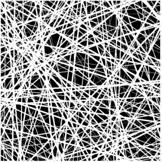
In the plane can be built a Boolean model on Poisson lines. For an isotropic lines network (…gure 1), and if A0 K is convex, we have, from equation (7):
T (K) = 1 exp L(A0 K) (9)
If A0
K is not convex, the integral of projected lengths over a line with the orientation varying between 0 and must be taken. If A0
and K are convex sets, we have L(A0
K) = L(A0
) + L(K). In the isotropic case and using for A0
a random disc with a random radius R (with expectation R) and for K is a disc with radius r, equation 9 becomes:
T (r) = 1 exp 2 (R + r) T (0) = P fx 2 Ag = 1 exp 2 R
which can be used to estimate and R , and to validate the model.
Figure 1: Simulation of a 2D Boolean model built on isotropic Poisson lines.
3.2 Random Fibers and Strata in 3D
3.2.1 Boolean model on Poisson planes
A Boolean model built on Poisson planes generates a structure with strata. On isotropic Poisson planes, we have for a convex set A0
K by application of equation (7):
T (K) = 1 exp M (A0 K) (10)
When A0
and K are convex sets, we have M (A0
K) = M (A0
) + M (K). If A0
K is not convex, T (K) is expressed as a function of the length l of the projection over the lines D!by T (K) = 1 exp
Z 2 ster
l(A0
(!) K(!)) d! . For instance if A0
is a random sphere with a random radius R (with expec-tation R) and K is a sphere with radius r, equation 10 becomes:
T (r) = 1 exp 4 (R + r)
T (0) = P fx 2 Ag = 1 exp 4 R
which can be used to estimate and R , and to validate the model. Figure 1 can be interpreted as a 2D section of a 3D Boolean model built on Poisson hyperplanes. It was shown in [8] that a two-components microstructure made of an in…nite superposition of random sets made of dilated isotropic Poisson planes with a large separation of scales owns extremal physical e¤ective properties (like electric conductivity, or elastic properties): when the highest conductivity is attributed to the dilated planes, the e¤ective conductivity is the upper Hashin-Shtrikman bound, while it is equal to the lower Hashin-Shtrikman bound, when a¤ecting the lower conductivity to the dilated planes.
3.2.2 Boolean model on Poisson lines
A Boolean model built on Poisson lines generates a …ber network, with possible overlaps of …bers. On isotropic Poisson lines, we have for a convex set A0 K T (K) = 1 exp 2S(A 0 K) (11) If A0
K is not convex, T (K) is expressed as a function of the area A of the projection over the planes ! by
T (K) = 1 exp Z
2 ster
A(A0(!) K(!)) d! (12)
If A0
is a random sphere with a random radius R (with expectation R and second moment E(R2)) and K is a sphere with radius r, equation 11 becomes: T (r) = 1 exp 2 2 (E(R 2) + 2rR + r2) T (0) = P fx 2 Ag = 1 exp 2 2 E(R 2)
which can be used to estimate , E(R2) and R , and to validate the model. A model of Poisson …bers parallel to a plane, and with a uniform distribution of orientations in the plane was used to model cellulosic …ber materials in [3]. In [17], non isotropic dilated Poisson lines were used to model and to optimize the acoustic absorption of nonwoven materials.
4
Fluctuations and RVE of the volume fraction
When operating on bounded domains, like 2D or 3D images of a material, one can be concerned by estimating the ‡uctuations of spatial average values Z(V ) of some random function Z(x) over the domain B with volume V . For instance if Z(x) is the indicator function of a random set A, Z(V ) is the area (in 2D) or the volume (in 3D) of the intersection A \ V . If Z(x) is some component of the strain …eld or of a stress …eld in an elastic medium, we can compute as well the average of these components over V , which are the standard way to de…ne and to estimate the e¤ective properties by homogenization [8, 9, 10].
When working on images of a material or on realizations of a random medium, it is common to consider the representativity of the volume fraction or of the e¤ective property estimated on a bounded domain of a microstruc-ture. Practically, we need to estimate the size of a so-called "Representative Volume Element" RVE [5, 8, 9, 10]. We address this problem by means of a probabilistic approach giving size-dependent intervals of con…dence, and based on the size e¤ect of the variance of the e¤ective properties of simula-tions of random media.
4.1 The integral range and scaling of the variance
We consider ‡uctuations of average values over di¤erent realizations of a random medium inside the domain B with the volume V . In Geostatistics [13], it is well known that for an ergodic stationary random function Z(x), with mathematical expectation E(Z), one can compute the variance D2Z(V ) of its average value Z(V ) over the volume V as a function of the central covariance function C(h) of Z(x) by : D2Z(V ) = 1 V2 Z B Z B C(x y) dxdy; (13) where
For a large specimen (with V A3), equation (13) can be expressed to the …rst order in 1=V as a function of the integral range in the space R3, A3, by
D2Z(V ) = DZ2A3 V ; (14) with A3= 1 D2 Z Z R3 C(h) dh; (15)
where DZ2 is the point variance of Z(x) (here estimated on simulations) and A3 is the integral range of the random function Z(x), de…ned when the integral in equations (13) and (15) is …nite. When Z(x) is the indicator function of the random set A, (14) provides the variance of the local volume fraction (in 3D) as a function of the point variance D2Z = p(1 p), p being the probability for a point x to belong to the random set A. When working in 2D, as was done to solve sampling problems in image analysis [5], the volume V is replaced by the surface area, and the integral range becomes A2 after integrating the covariance in the 2D space R2 in equation 15. The asymptotic scaling law (14) is valid for an additive variable Z over the region of interest B. To estimate the e¤ective elasticity or permittivity tensors from simulations, we have to compute the spatial average stress h i and strain h"i (elastic case) or electric displacement hDi and electrical …eld hEi. For the applied boundary conditions, the local modulus is obtained from the estimations of a scalar, namely the average in the domain B of the stress, strain, electric displacement, or electric …eld. Therefore the variance of the local e¤ective property follows the equation (14) when the integral range A3 of the relevant …eld is known. Since the theoretical covariance of the …elds ( or ") is not available, the integral range can be estimated according to the procedure proposed by G. Matheron for any random function [15]: working with realizations of Z(x) on domains B with an increasing volume V (or in the present case considering subdomains of large simulations, with a wide range of sizes), the parameter A3 is estimated by …tting the obtained variance according to the expression (14).
Some typical microstructures with long range correlations, like dilated Poisson hyperplanes mentionned in section 3.2.1 or like dilated Poisson lines in 3D have an in…nite integral range [6, 7], so that the computation of the variance D2
Z(V ) of equation (14) cannot be used anymore. In this situation, a scaling law by a power < 1 was suggested [12], and used in various applications where a coe¢cient close to 1 was empirically estimated [2, 10]. With this scaling law, the variance becomes
DZ2(V ) = D2Z A3
V ; (16)
where the volume A3 is no more the integral of the central covariance func-tion C(h), but is still homogeneous to a microstructural volume. We will
show in section 5, that such scaling power laws appear in the case of Boolean models built on the linear Poisson varieties.
4.2 Practical determination of the size of the RVE
The size of a RVE can be de…ned for a physical property Z, a contrast, and a given precision in the estimation of the e¤ective properties depending on the number n of realizations that are available. By means of a stan-dard statistical approach, the absolute error abs and the relative error rela on the mean value obtained with n independent realizations of volume V are deduced from the 95% interval of con…dence by:
abs= 2DZ(V ) p n ; rela= abs Z = 2DZ(V ) Zpn : (17)
The size of the RVE can now be de…ned as the volume for which for in-stance n = 1 realization (as a result of an ergodicity assumption on the microstructure) is necessary to estimate the mean property Z with a rela-tive error (for instance rela= 1%), provided we know the variance D2Z(V ) from the asymptotic scaling law (14) or (16). Alternatively, we can decide to operate on smaller volumes (provided no bias is introduced by the boundary conditions), and consider n realizations to obtain the same relative error. This methodology was applied to the elastic properties and thermal conduc-tivity of a Voronoï mosaic [10], of materials from food industry [11], or of Boolean models of spheres [18].
5
Scaling of the variance of the Boolean random
varieties
5.1 Boolean model on Poisson varieties in Rn
We consider a convex domain K in Rn, with Lebesgue measure
n(K). Deriving the asymptotic expression of the local fraction (with average p) from the covariance (8) in expression (13) is not an easy task. The scaling law of the variance (16) can be directly obtained for the Boolean model built on isotropic Poisson varieties Vk from the properties of the Poisson point process. We have the following result.
Proposition 6 In Rn, the variance D2
Z(K) of the local fraction Z = n (A\K)
n(K)
of a Boolean model built on isotropic Poisson varieties of dimension k (k = 0; 1; :::; n 1) Vk, is expressed by
D2Z(K) = p(1 p) Ak n(K)
n k n
the scaling exponent being = n kn . As particular cases, Poisson points (k = 0) give the standard Boolean model with a …nite integral range and = 1, Poisson lines (k = 1) generate Poisson …bers with = n 1n , and Poisson hyperplanes (k = n 1) provide Poisson strata with = 1n.
Proof. Consider isotropic varieties Vk with dimension k and intensity k. From proposition 3, the number of varieties hit by K follows a Poisson distribution with average and variance proportional to kWk(K). To express the scaling law of the variance D2
Z(K), we consider the limiting case of a low intensity k in expression (5) for large K as compared to the primary grain A0
( n(A0
) << n(K)), so that to …rst order Wk(K) Wk(A0 K). For a given realization of Vk, the measure n(A \ K) is proportional to k(Vk \ K). As a result of the ergodicity of the random varieties Vk,for large K, k(Vk\ K) converges towards the mathematical expectation of the measure of random sections of K, Ef k(Vk\ K)g. Its value can be deduced from the Crofton formula given in [14], p. 82. We get, making use of (5):
Ef k(Vk\ K)g = n (K) Z
n k(K(!)) d! The local volume fraction of A, n(A\K)
n(K) has an expectation proportional to
kWk(K)Z 1
n k(K(!)) d!
k and a variance proportional to
kWk(K) 1 Z n k(K(!)) d! 2 1 Wk(K) 1 n(K) n k n
It turns out that the most penalizing situation with respect to the scaling of the variance is the case of Poisson strata, with a very slow decrease of the variance with the volume of the sample K, with = n1.
It is di¢cult to give equivalent results for general non-isotropic models. Instead, we will give below some speci…c examples useful for applications in 2D and in 3D.
5.2 Random …bers in 2D
For isotropic Boolean …bers in 2D, the scaling exponent is = 12. Note that in that case the Poisson varieties are Poisson lines, which are at the same time lines and hyperplanes in R2.
An instructive and extreme anisotropic case is obtained for parallel Poisson lines, with the intensity 1(d ) = 1 ( 0)d , 0 being the
orientation of the lines. For a sample K made of a rectangle with an edge L orthogonal to 0, and an edge l parallel to 0. The number of lines hitting K is a Poisson variable with average and variance 1L. The average of the local area fraction of A is proportional to 1LLll =
1LL1 and its variance is proportional to 1LL12 = 1
L. The length l plays no role in the variance, which is inversely proportional to L. In that case, 1D samples orthogonal to 0 produce the same scaling of the variance. This can be explained by the fact that the 1D sections of the model orthogonal to 0 are a standard one-dimensional Boolean model with a …nite integral range, showing a standard scaling of the variance in 1D.
5.3 Random …bers in 3D
For isotropic Boolean …bers in 3D, the scaling exponent is = 23. This exponent was recovered for the volume fraction from numerical simu-lations [4]. In the case of …bers with a …nite length, an intermediary situation will occur, and a scaling coe¢cient 23 6 61, depending on the size of the specimen is expected ( ' 23 for small specimens, and ' 1 for large samples). Simulations of various random networks of …nite …bers having a length of the order of the size of the samples, and with various distributions of [1], gave ' 0:66 0:87 for the volume fraction. For Simulations of the elastic properties and of the conduc-tivity of 3D random …ber networks by …nite elements [4] or by FFT [1] provide an empirical scaling law of the variance close to the theoretical one obtained for the volume fraction. This is expected, as a result of a high correlation between the elastic or thermal …elds and the indicator function of the random set A.
An extreme case of anisotropy is given for …bers parallel to a direction 0, providing a standard 2D Boolean model in planes orthogonal to 0. Consider for K a paralleliped with a face orthogonal to the direction 0 (with area S), and an edge parallel to the direction 0(with length l). The number of Poisson lines hitting K is a Poisson variable with parameter 1S, and 2D sections of A generate a standard 2D Boolean model. The average of the local volume fraction of A is proportional to 1SSll = 1SS1 and its variance is proportional to 1SS12 =
1
S. As in 1D, the length l plays no role in the variance, which is inversely proportional to S. The same scaling is obtained for 2D sections in planes orthogonal to the direction 0. This was observed on a silica …bers composite, for the ‡uctuations of the area fraction and of the elastic and thermal …elds, calculated by …nite elements on polished sections of the composite [16]. Planar sections parallel to 0 generate a 2D model of Boolean …bers. The variance is proportional to 1
being the length of the edge orthogonal to 0, the edge parallel to the …bers playing no roles. In this situation, one dimensional sections orthogonal to 0, give the same scaling law for the variance, that is decreasing much slower than for transverse sections or for the isotopic model.
It is possible to model a random woven composite by a network of random …bers with a set of orientations, for instance two or three orthogonal orientations 1, 2, 3, and corresponding intensities 1, 2, 3. Consider for K a paralleliped with a face orthogonal to the direction 1(with area S1), and faces orthogonal to direction 2 (with area S2) and to direction 3 (with area S3). The lengths of the edges in direction i are Li (i = 1; 2; 3), so that S1 = L2L3, S2 = L1L3 and S3 = L2L1. In the case of two orthogonal directions 1, 2, the variance scales as 1
S1 + 2
S2, while for three orthogonal orientations, it
scales as 1
S1 + 2
S2 + 3
S3. For a cube, an overall scaling in S is recovered
with = 1 + 2+ 3, which still gives a scaling exponent = 23. The microstructure can also be sampled by planar probes K. For two directions of …bers 1, 2 and cuts orthogonal to direction 1, the variance scales as 1
S1 + 2
L2. For cuts parallel to the plane de…ned
by orientations 1, 2 the variance scales as L11 + 2
L2, which is the
most penalizing situations. These results extend to three orthogonal orientations, with a variance scaling as 1
S1+ 2
L2+ 3
L3 for cuts orthogonal
to direction 1, which are therefore parallel to the plane de…ned by directions 2, 3.
Some …brous materials, like cellulosic …brous media [3], are isotropic transverse: …bers are parallel to a reference plane, orthogonal to some direction 3, with a uniform distribution of orientations in this plane. The number of Poisson line hit by K follows a Poisson distribution with parameter (L1+ L2)L3, and the variance of the local volume fraction scales as (L
1+L2)L3. Planar sections with area S of this model
orthogonal to the direction 3 generate a 2D isotropic Boolean model of …bers with the scaling exponent = 12 for S1, as in 5.2.
Projections of 3D Boolean …bers networks on a plane generate various standard models with the corresponding scaling laws. Any projection of the isotropic network, or a projection of transverse isotropic …bers in a plane parallel to …bers [3] are 2D isotropic Boolean …bers with he scaling exponent = 12 for S1 as in 5.2. The projection of parallel …bers in a plane parallel to …bers generates 2D Boolean parallel …bers, with a variance scaling as L1, L being the length of the edge of the section orthogonal to …bers. The projection of parallel …bers in a plane orthogonal to …bers generates standard 2D Boolean model with
a scaling of the variance in S1. This models appear by observation of thick slides of …brous networks, as obtained by optical confocal microscopy [3], or from transmission electron microscopy.
5.4 Random strata in 3D
For isotropic Boolean strata in 3D, the scaling exponent is = 13. This decrease of the variance with size is much slower than the case of a …nite integral range. When considering random media with a nonlinear behaviour, like for instance a viscoplastic material, a strong localisation of strains resulting in shear bands is expected. This gen-erates long range correlations of the …elds, that might be modeled by Boolean strata in 3D, and scaling laws similar to the dilated Poisson hyperplanes (with a scaling exponent close to 13) might be recovered, so that a slow convergence towards the e¤ective properties should be observed on numerical simulations with increasing sizes.
A layered medium, generated by parallel hyperplanes, orthogonal to a reference direction 0. corresponds to an extremal anisotropy. Con-sider for K a paralleliped with a face orthogonal to the direction 0 (with area S). The length of the edge parallel to 0 is L. The number of planes hit by L is a Poisson variable with parameter L. The local volume fraction has an expectation equal to LVS = and its variance is proportional to L VS 2 = L. For this situation, there is no e¤ect of the surface S, and plane sections parallel to the direction 0 gives the same scaling of the variance.
Another instructive case is obtained by isotropic hyperplanes parallel to a given direction 0. Consider for K a paralleliped with a face orthogonal to the direction 0 (with perimeter L and area S). The number of Poisson planes hit by K follows a Poisson distribution with parameter L. If the length of K in the direction parallel to 0is L, the local volume fraction has an expectation equal to LLVL = , and its variance is proportional to L LL
V 2
S1=2
V1=3. Planar sections
(or equivalently projections) orthogonal to 0 generate isotropic 2D Boolean …bers, with a variance scaling in
S1=2. Vertical planar sections,
parallel to 0 (with a horizontal edge L) generate parallel 2D Boolean …bers, with a variance scaling in L, the size of the vertical edge playing no role in the variance.
As for …bers, It is possible to model a random woven composite by a network of random strata with a set of orientations, for instance two or three orthogonal orientations 1, 2, 3. Consider for K a paralleliped with edges parallel to these orientations, and lengths L1,
L2, and L3. The variance scales as L11 + 2
L2 + 3
L3. When K is a cube
with edge L, the variance scales as 1+ 2+ 3
L .
6
Conclusion
Boolean random varieties generate random media with in…nite range corre-lations. As a consequence, non standard scaling laws of the variance of the local volume fraction with the volume of domains K are predicted. These laws are out of reach of a standard statistical approach. We have theoreti-cally shown that on a large scale, a the variance of the local volume fraction decreases with power laws of the volume of K. The exponent is equal to
2
3 for Boolean …bers in 3D, and 13 for Boolean strata in 3D. When working in 2D, the scaling exponent of Boolean …bers is equal to 12. Therefore the decrease of the variance with the scale is much slower for these models as compared to situations with a …nite integral range, like the standard Boolean model built on a Poisson point process with compact primary grains, and larger RVE are expected for the estimation of the volume fraction. These laws are expected to hold when using numerical simulations to predict the e¤ective properties of such random media, as already empirically observed for the conductivity or for the elastic properties of random …bers models. The obtained scaling laws in various cases, including anisotropic orientations of the Boolean …bers or strata, can help to design optimal sampling schemes with respect to minimizing the variance of estimation.
References
[1] H. Altendorf, 3D Morphological analysis and modeling of random …ber networks, PhD thesis, Mines ParisTech, November 2011.
[2] Cailletaud G., Jeulin D., Rolland Ph. (1994) Size e¤ect on elastic prop-erties of random composites, Engineering computations, vol 11, N 2, pp. 99-110.
[3] Delisée Ch., Jeulin D., Michaud F. (2001) Caractérisation mor-phologique et porosité en 3D de matériaux …breux cellulosiques, C.R. Académie des Sciences de Paris, t. 329, Série II b, pp. 179-185, 2001. [4] Dirrenberger, S. Forest, D. Jeulin, M. Faessel, F. Willot F. (2011)
Modélisation de milieux …breux aléatoires enchevêtrés et estimation de VER, Communication to Mecamat (Sophia Antipolis, 11 May 2011), in preparation.
[5] Hersant T., Jeulin D. (1976) L’échantillonnage dans les analyses quan-titatives d’images. Exemples d’application aux mesures des teneurs de
phases dans les agglomérés et des inclusions dans les aciers, Mémoires et Etudes Scienti…ques de la Revue de Métallurgie, 73, 503.
[6] Jeulin D. Modèles Morphologiques de Structures Aléatoires et de Changement d’Echelle. Thèse de Doctorat d’Etat ès Sciences Physiques, Université de Caen, 25 Avril 1991.
[7] Jeulin D. (1991) Modèles de Fonctions Aléatoires multivariables. Sci. Terre; 30: 225-256.
[8] Jeulin D. (2001) Random Structure Models for Homogenization and Fracture Statistics, in Mechanics of Random and Multiscale Microstruc-tures, ed. by D. Jeulin and M. Ostoja-Starzewski (CISM Lecture Notes N 430, Springer Verlag), pp. 33-91.
[9] Jeulin D. (2005) Random Structures in Physics, in: "Space, Structure and Randomness", Contributions in Honor of Georges Matheron in the Fields of Geostatistics, Random Sets, and Mathematical Morphology; Series: Lecture Notes in Statistics, Vol. 183, Bilodeau M., Meyer F., Schmitt M. (Eds.), 2005, XIV, Springer-Verlag, pp. 183-222.
[10] Kanit T., Forest S., Galliet I., Mounoury V., Jeulin D. (2003) Deter-mination of the size of the representative volume element for random composites: statistical and numerical approach, International Journal of solids and structures, Vol. 40, pp. 3647-3679.
[11] T. Kanit, F. N’Guyen, S. Forest, D. Jeulin, M. Reed, S., Singleton, Apparent and e¤ective physical properties of heterogeneous materials: Representativity of samples of two materials from food industry, Com-put. Methods Appl. Mech. Eng. 195 (2006) 3960–3982.
[12] C. Lantuejoul, Ergodicity and integral range, Journal of Microscopy 1991, 161:387-403.
[13] G. Matheron, The theory of regionalized variables and its applications, Paris School of Mines publications 1971.
[14] Matheron G. (1975) Random sets and Integral Geometry, J. Wiley, N.Y.
[15] G. Matheron, Estimating and Choosing, Springer Verlag, Berlin (1989). [16] Oumarou M., Jeulin D., Renard J. (2011) Etude statistique multi-échelle du comportement élastique et thermique d’un composite ther-moplastique, Revue des composites et des matériaux avancés, Vol. 21, N 2 , pp. 221-254.
[17] Schladitz K., Peters S., Reinel-Bitzer D., Wiegmann A., Ohser J., De-sign of acoustic trim based on geometric modeling and ‡ow simulation for non-woven, Computational Materials Science 38 (2006) 56–66. [18] F. Willot, D. Jeulin, Elastic behavior of composites containing Boolean
random sets of inhomogeneities, International Journal of Engineering Sciences, Vol. 47 (2009) 313-324.