HAL Id: hal-00267621
https://hal.archives-ouvertes.fr/hal-00267621
Submitted on 27 Mar 2008
HAL is a multi-disciplinary open access
archive for the deposit and dissemination of
sci-entific research documents, whether they are
pub-lished or not. The documents may come from
teaching and research institutions in France or
abroad, or from public or private research centers.
L’archive ouverte pluridisciplinaire HAL, est
destinée au dépôt et à la diffusion de documents
scientifiques de niveau recherche, publiés ou non,
émanant des établissements d’enseignement et de
recherche français ou étrangers, des laboratoires
publics ou privés.
The Mojette Transform: The First Ten Years
Jean-Pierre Guédon, Nicolas Normand
To cite this version:
Jean-Pierre Guédon, Nicolas Normand. The Mojette Transform: The First Ten Years. Discrete
Geometry for Computer Imagery, Apr 2005, Poitiers, France. pp.79-91, �10.1007/b135490�.
�hal-00267621�
The Mojette Transform: The First Ten Years
JeanPierre Gu´edon and Nicolas NormandIRCCyN/IVC UMR CNRS 6597
Abstract. In this paper the Mojette transforms class is described. After recalling the birth of the Mojette transform, the Dirac Mojette transform is recalled with its basic properties. Generalizations to spline transform and to nD Mojette transform are also recalled. Applications of the Mojette transform demon-strate the power of frame description instead of basis in order to match different goals ranging from image coding, watermarking, discrete tomography, transmission and distributed storage. Finally, new insights for the future trends of the Mojette transform are sketched.
@inproceedings{guedon2005dgci,
Author = {Gu{\’e}don, JeanPierre and Normand, Nicolas}, Booktitle = {Discrete Geometry for Computer Imagery}, Date = {2005-04},
Doi = {10.1007/b135490},
Editor = {Andres, {\’E}ric and Damiand, Guillaume and Lienhardt, Pascal}, Isbn = {3-540-25513-3},
Month = apr, Pages = {79-91},
Publisher = {Springer Berlin / Heidelberg}, Series = {Lecture Notes in Computer Science},
Title = {The {M}ojette Transform: The First Ten Years}, Volume = {3429},
Year = {2005}}
THE MOJETTE TRANSFORM:
the First Ten Years
JeanPierre Gu´edon and Nicolas Normand
Laboratoire IRCCyN, Team Image & Video Communications CNRS UMR 6795, ´
Ecole polytechnique de l’Universit´e de Nantes La Chantrerie Rue Christian Pauc, BP 50609, F-44306 Nantes cedex 3{firstname.lastname}polytech.univ-nantes.fr
Abstract. In this paper the Mojette transforms class is described. After recalling the birth of the Mojette transform, the Dirac Mojette transform is recalled with its basic properties. Generalizations to spline transform and to nD Mojette transform are also recalled. Applications of the Mo-jette transform demonstrate the power of frame description instead of basis in order to match different goals ranging from image coding, wa-termarking, discrete tomography, transmission and distributed storage. Finally, new insights for the future trends of the Mojette transform are sketched.
1
Introduction
1.1 The Word ”Mojette”
”Mojette” is a well known word in Poitiers; in old french, it describes the class of white beans. Until recently, these white beans were the standard tool for a child to start computing additions and subtractions. They were also used for computing the number of victories for card games like ”Aluette” still played with middle age spanish cards. Mojette is the name of our transform to remember first that when only adds are invoked, the computations can be easily made, second that by sharing the information pot each player will get a part of it. 1.2 The First Papers
The first paper on the Mojette transform has been published in 1995 after one year of hard work. At the moment, we were looking for something that we still did not find: a discrete mathematical tool that can split the Fourier plane into radial and angular sectors. The initial application was the psychovisual image encoding that mimics the human channelized vision. Hopefully, what we found was so much practical that many applications did appeared later on. The first talk on the Mojette transform (denoted MT in the following) was published in SPIE Visual Communications and Image Processing [8]. The fact that a novel transform was welcomed by the community was of prime importance to continue this kind of research. Even if all the theory was not yet there, the structure of the transform was already explained by its first inverse version using a recursive implementation. The first laboratory talk was given on June 22d 1995.
1.3 Related Works
The first two precursors of the Mojette transform were Myron Katz and Gabor Herman. They were both looking at discrete geometric tools to properly inverse the Radon transform at the beginning of the X-ray scan. The concept of discrete angles that we used later on in the MT was taken from Myron Katz’ work [12]. Gabor Herman presented iterative algorithms to solve the equation f = Rp where f is the image, R is a discrete Radon projection operator and p is the set of projections obtained with a constant bin width [11]. In this regard, mixing both works gives the Mojette transform.
The mood for a discrete Radon transform use only came back in the nineties; except for pioneer works as Attila Kuba who was starting to see the generality of the problem using discrete geometry in 1984 [13]. Gu´edon [9, 7] starts with a spline version of the Radon transform in order to fill the gap between discrete and continuous points of view. L. Dorst added a major point by linking the Radon (or slope) transform to mathematical morphology [3] as independently we did obtained our first reconstruction theorem by this link to the two pixel structuring element. Notice that a big step has been made in 1999 when Jean-Marc Chassery did organize a workshop on discrete tomography that was using discrete geometry for mixing the kind of solutions for a given polyominos problem [2] with the complexity of others very close problems [5, 6]. However, it must be clear here that the Mojette transform does not exactly belongs to the ”discrete tomography” community in the sense the word was defined by Larry Shepp in 1994, i.e. reconstructing an object from two to four projections.
A novel situation arises now, when many and very interesting papers are published to express different properties of transforms very close to the MT as [22] and unread papers come back to the community as [14].
1.4 Paper Organization
The paper is split into theoretical results and applications. The second section of the paper reviews the properties of the Mojette transform. The simple definition of the direct Mojette transform (that will be described by Dirac-Mojette after-wards) is first presented and its fast inversion (same order of complexity than the direct operator) follows. The strong relationships with mathematical mor-phology are then presented because they constitute both the core of the proofs of the reconstruction theorems we obtained and the geometric way to cope with the transform. The generalization to spline Mojette transform and other kernels are then presented to show the power of the relationships between continuous and discrete words. In other words, this link allows for translating various prob-lems such as tomography into the discrete geometry world. Finally, extensions to higher dimensions demonstrate two notions : the order of complexity of the transform is still linear in the number of pixels, voxels, ixels (information ele-ments) and linear into the number of hyperplanes. The third section present the variety of applications already found for the Mojette transform. The key point that is used here is the frame description notion (instead of the classical vectorial
basis). Its first obvious success (because of its direct implementation) was to use the Mojette transform as a tool for multiple description which has evolved to a kind of new standard for communications [17]. A step further in this area was to add the hierarchical (or multiresolution) data description with the concept of multi-layer buffering. Another completely different application was to mas-ter the noise properties into the Mojette domain in order to allows the Mojette transform for tomographic reconstruction. Even if this sounds obvious from the Radon inheritance, this works is the last one we were able to perform. Back to the image domain, the Mojette transform has been successfully implemented to solve for new techniques as watermarking as well as texture analysis for image and video as presented in this section. The final part of the paper gives some insights for the next ten years.
2
Basic Mojette Transform Properties
2.1 Direct and Inverse Dirac-Mojette Transform
The mojette transform is derived from the Radon transform [20]. The 2-D trans-formed domain consists in projections (in the Radon sense) where each calcu-lated element called a bin is the sum of ixel values. However, from an original block f(k, l) of information elements (denoted ixel for information element), the Mojette transform gives a linear set of projections projθ(m) only for specific
angles of the form θ = atan(q/p) where p ∈ Z, q ∈ Z+ and are relatively prime
(GCD(p, q) = 1). The Mojette transform set is defined by Mf(k, l) as a set of
I projections Mp,qf (k, l), where (k, l) belongs to the ixels block and ∆(m) = 1
if m = 0, 0 otherwise, as follows:
M f ={Mpi,qif, i = 1, . . . , I} = {projpi,qi, i = 1, . . . , I} (1)
Mp,qf (k, l) = projp,q(m) = projθ(m) = f(k, l)∆(m + qk − pl), (2)
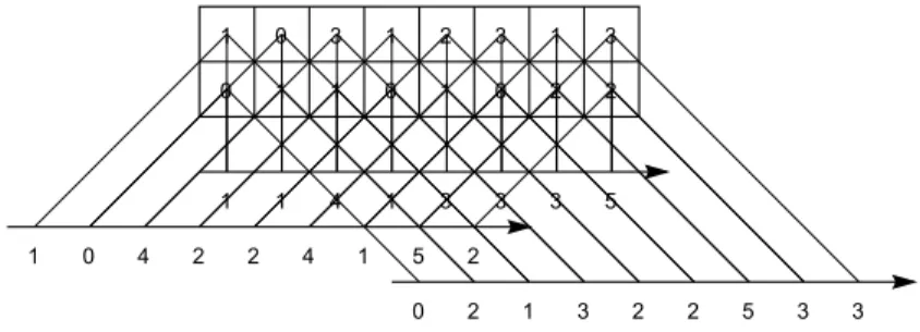
A bin value is then simply the summation of every ixel intersecting the line
m = −qk + pl. As described in Fig. 1, the major difference with the Radon
transform is that the bin spacing on a projection depends on the projection angle.
The well-posed nature of this linear transform and its explicit discrete nature were the reason of the new name not to confuse with the numerous regularized versions of the Radon transform (ill-posed inverse operator). A direct conse-quence of this sampling is that the number of bins of the projection indexed by (p, q) depends both of the projection angle and of the block dimensions. For instance, a P × Q rectangular block has its (p, q) projection composed of B bins with B = (Q − 1)|p| + (P − 1)|q| + 1. The order of complexity of the direct transform is obviously O(IN) i.e. linear in the number of (p)ixels N and linear in the number of projections I.
The inverse transform can be implemented with the same order of complexity. This is an important characteristic of the Mojette transform which comes from the underlying mathematical morphology properties as described in the next
Fig. 1. Mojette Transform of a 3× 3 f(k,l) lattice
paragraph. To get such a result, the reader has to pay attention to the projection of the ”corners” of the shape: they exhibit some one to one ixel-bin relationships. Thus, these specific bins can be exactly backprojected in the image as soon as we keep for each bin the number of contributed ixels during the inverse transform. The tool for the proof of this algorithm (given in [15]) is now presented. 2.2 Mathematical Morphology
Reconstruction conditions were demonstrated for any convex image [15] by as-sociating a projection angle (p,q) with a 2 pixels structuring element (2PSE) as a point couple {O, (p, q)} giving the same direction axis. The set of ixels that are projected in one bin m is the intersection of the image with the (p, q) − line defined by: −qk + pl = m. If the image is convex, this set is connected relative to the (p, q)-neighborhood (all ixels are reachable from the others using (p, q) displacements). Thus, an opening (an erosion followed by a dilation) with the 2PSE {O, (p, q)} will empty the set if it is composed of exactly one ixel but will leave it unchanged in all other cases. The back projection in direction (p, q), by removing all ixels in a one to one correspondence with a bin, results in the opening of the image with the 2PSE:
I! = I ◦ {O, (p, q)} .
An ixel disappears from I only if it has no (p, q)-neighbor.
The final reconstruction result is not affected by the order bins are back projected. So the overall reconstruction can be viewed as an iterative series of openings with the 2PSEs:
Ik+1= Ik◦ {O, (p1, q1)} ◦ . . . ◦ {O, (pI, qI)} .
The reconstruction stops if no ixels can be removed by any projection (Ik+1=
(p, q)-neighbor in every (p, q) direction. The smallest non-null image with that property is built by the series of dilations with the 2PSEs.
The reconstructibility criteria of Katz finds here another expression only using dilations. A convex image is not reconstructible if and only if the dila-tion result by 2PSE is not included in the image support (even if one pixel is concerned). This general result is expressed in the following theorem by the equivalence of two statements.
Theorem 1. Both propositions are equivalent
– f(k, l) defined on the convex G is reconstructible by {projpi,qi, i = 1, . . . , I};
– R constructed by I dilations set {{O, (pi, qi)}, i = 1, . . . , I} is not included
in G.
Corollary 1. Both propositions are equivalent – G is reconstructible by {projpi,qi, i = 1, . . . , I};
– the erosion of G by R is null.
Proj-1,1 0 1 1 0 5 2 0 3 6 5 2 2 0 4 0 2 3 4 3 2 1 0 1 1 0 2 6 3 2 2 0 4 2 3 3 3 2 1 0 0 5 2 1 4 0 2 3 0 Proj1, 0 Proj1,1 Proj-1,1 Proj-2,1 2 3 1 3 1 0 2 2 1 0 3 1 0 1 1 0 3 5 5 2 0 4 1 2 6 2 0 0 2 6 3 2 2 0 0 0 2 1 2 2 2 2 1 1 0 2 2 3 3 2 1 1 4 4 4 0 1 3 3 3 2 1 image support structuring elements 0 0 3 2 1 4 0 2 3 0 Proj-2,1 2 3 1 3 1 0 2 2 1 0 3 1 0 1 1 0 0 0 1 1 2 2 2 2 1 1 1
Fig. 2. Reconstructibility of a convex image
This inversion criterion is an extension of Katz’ criterion for rectangular images. In that particular case, R can be included in the image if its width (1 + !i|pi|) and height (1 +!i|qi|) are respectively smaller than the width P
and height Q of the image. Thus, for a P × Q image, a complete reconstruction is achievable if [12]: P ≤" i |pi| or Q ≤ " i |qi| (3)
2.3 Spline Mojette Transform
The previous Mojette transform is denoted Dirac-Mojette transform because the underlying 2D ixel representation is a Dirac field:
f (x, y) ="
k
"
l
However, very similar angles like (p, q) = (1, 1) and (p, q) = (30, 29) will do not have similar bin values: a direct inter-correlation computation between the two projections will be poor because the number of bins and the number of pixels contributing to each bin will be very different. However, Philipp´e and Gu´edon [19] have shown that the autocorrelation of the Mojette projection corresponds to the projection of the autocorrelation of the image.
Summing ixel intensities weighted by the relative length of the ray inside each ixel, defines the spline0-Mojette transform. The corresponding continuous
image is given by:
f (x, y) ="
k
"
l
f (k, l)β0(x − k)β0(y − l) , (5)
where β0(x) = 1 when |x| < 12, β0(12) = 12 and 0 elsewhere.
It can be simply shown that the spline0-Mojette transform corresponds to
the filtering of the Dirac-Mojette transform with a finite impulse response (FIR) filter. The FIR filter definition wp,q(m) corresponds to a trapezoidal shape, i.e.
the projection of the shape of the ixel (a square in 2D) as described in [10].
M0f = [MDf ]∗ wp,q , (6)
Where the kernel w can always be decomposed with small filters composed of unitary values. In other words only additions can be used for implementation of this convolution and the recursive filter that implements the inverse operator (going from spline0to Dirac Mojette data) will only use subtractions.
The generalization to higher spline order Mojette transform follows the same pattern. From a βn spline definition of the original function given as:
f (x, y) ="
k
"
l
f (k, l)βn(x − k)βn(y − l) , (7)
with βn(x) = βn−1(x) ∗ β0(x), the splinen-Mojette transform is defined as:
Mnf (k, l) = [Mn−1f ]∗ wp,q(b) . (8)
The main originating reason to use spline functions instead of Dirac fields is to complied with the generalization of the well-known Shannon-Wittaker sampling theorem obtained by Unser and AlDroubi [1, 23–25]. This theorem allows to combine the projection decomposition with other image needs like wavelet or geometric (e.g. rotation) operators.
The main use of spline Mojette transform is to introduce a controlled re-dundancy inside each projection via the kernel w. Direct applications to error correcting codes have already been obtained [21] in the presence of noise in-side the projection data. This intra-redundancy can be managed at the same time that the inter projections redundancy to answer consistency of distributed information projections as shown in the applications.
2.4 nD Mojette Transform
Going from 2D results to 3D then nD is an indefectible temptation to generalize the obtained results. This was done by still considering the Mojette transform as giving (n − 1)D hyperplanes from the nD discrete hypervolume. It can be easily shown that from N ixels distributed inside a convex set of dimension n and a choice of I hyperplanes, the direct and inverse Mojette transform still exhibit a complexity order of O(IN). This is quite obvious for the direct transform. The way of having this very low cost algorithm for the inverse transform is to use the same mapping than previously used in 2D between ixels and bins. As a matter of fact, this mapping is dimension independent.
Another result that can be seen as independent of the dimension is the dis-crete central slice theorem (CST). The continuous version of the CST has been extensively used for Radon inversion as well as for image processing. It says that the 1D Fourier transform of a projection of angle θ equals the slice of the 2D Fourier transform of the image at angle θ + π/2. The discrete version of this the-orem was established in 2D by Dudgeon and Mersereau using the Z transform [4]. It has been checked with the 2D Mojette transform and extended to higher dimensions in a straightforward manner [26].
2.5 Mojette Transform and Redundancy
The Mojette transform matrix M is only filled by 1 and 0 values. Only addi-tions and subtracaddi-tions are required for M and M∗. It is also the case for M−1
with the inverse Transform algorithm for exact values [15]. The matrix M∗M is
Toeplitz-block-Toeplitz. Since only the additive group structure is needed for its definition, replacing the natural addition by modulus addition will not change any property of the transform. This can be done as soon as the initial values of the ixels are quantized onto an interval [0, 2b[ where b represents the number of bits of an ixel. In this case, a bin will belong to the same interval (by modulus addition), so do the reconstructed ixel. This represents an important matter for not having an overbinary representation in the Mojette domain as well as to use the same type of elements in both domains.
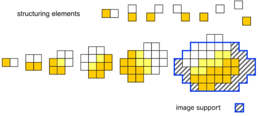
The computation of a redundancy factor as Red = #Bins/#Ixels − 1, gives the true weight for managing a frame. However, this Red indicator does not explain at all the stability of the transform under inconsistency (e.g. noise) considerations. In such a case, the number of projections as well as the dif-ference between the initial shape and the dilations of two ixel structuring el-ements (2ISE) will better explain the power of recovering inconsistency. For instance, for a 5 × 5 convex, the sets S0 = {(5, 3)}, S1 = {(3, 2), (2, 1)} and
S2= {(1, 0), (−1, 1), (1, 1), (2, 1)} all fulfill the reconstruction conditions and give
Red= 8/25. The corresponding reconstructed shapes are illustrated in Fig. 3. The importance of splitting the initial information into (projection) pieces can be pictured as in the previous figure or computed as the conditioning factor of the matrix M ∗ M. In this example, when the first degenerated information set gets a false bin value it will not been detected at the reconstruction step, the second set will detect the error but not correct it as the third set does.
8 DGCI 2005
The computation of a redundancy factor as Red= #Bins/ #Ixels – 1, gives the true weight for managing a frame. However, this Red indicator does not explain at all the stability of the transform under inconsistency (e.g. noise) considerations. In such a case, the number of projections as well as the difference between the initial shape and the dilations of two ixel structuring elements (2ISE) will be better explained the power of recovering inconsistency. For instance, for a 5x5 convex, the sets S0={(5,3)}, S1={(3,2),(2,1)} and S2={(1,0),(-1,1),(1,1),(2,1)} all fullfil the reconstruction conditions and give Red= 8/25. The corresponding reconstructed shapes are illustrated in figure 2.
Figure 2 : Redundancy of three sets of projections under a 5x5 f(k,l) lattice
The importance of splitting the initial information into (projection) pieces can be pictured as in the previous figure or computed as the conditionning factor of the matrix M*M. In this example, when the first degenerated information set gets a false bin value it will not been detected at the reconstruction step, the second set will detect the error but not correct it as the third set does.
2.7. MOJETTE TRANSFORM AND FAREY SERIES
nn
3. Applications
The power of the Mojette transform lies in it abilities to manage inconsistency. The first way to have inconsistent data is to have not enough data whereas it exists some intrinsic correlation inside the data as shown in the last paragraph of section two. In this case, only some partial exact descriptions of the information are available: this corresponds to the multiple description problem. This information can also already be sorted in an hierarchical manner and treated with the same formilsm through the use of the Mojette transform. The second case is the shape description problem Fig. 3. Redundancy of three sets of projections under a 5× 5 f(k, l) lattice
3
Applications
The power of the Mojette transform lies in it abilities to manage inconsistency. The first way to have inconsistent data is to have not enough data whereas it exists some intrinsic correlation inside the data as shown in the last paragraph of section two. In this case, only some partial exact descriptions of the infor-mation are available: this corresponds to the multiple description problem. This information can also already be sorted in an hierarchical manner and treated with the same formalism through the use of the Mojette transform. The second case is the shape description problem through some of its projections, where the Mojette transform becomes a geometric tool when allied with the mathematical morphology. The third case of inconsistent data arises when metadata is added inside the data as for the watermarking techniques. Then the two coexisting kinds of data must have different behaviors (one must be shown while the other should lie under the expressed data until a specific algorithm can reveal it. The fourth case is when enough projections are available but are corrupted by noise such that only an approximation can be computed as for tomography.
3.1 The Use of Redundancy: the Multiple Description Tool
The multiple description problem arises in the seventies and was studied by Ozarow and others as an information theory problem for telephony over two channels [16]. It has been developed for a decade for Internet transmission and now for distributed storage. The paradigm is as follows: given an initial infor-mation set, computes I different descriptions such that for a lower number of descriptions there is still always an approximation that can be computed and used usually for real-time considerations.
Many kind of solutions have been employed ranging from Turbo-codes, Solo-mon codes, Tornado codes and of course Mojette projections. The major prop-erty of these codes is generally to be Minimum Description Separable (denoted MDS), that is without redundancy as for Solomon or Tornado codes or (1 + &)-MDS as for the Mojette codes demonstrated by Parrein [17]. The price of the redundancy can be easily paid to gain much more flexibility in the design of the code (which means to choose a pair of shape and set of projections) whereas Solomon codes must be only determined from Galois field GF (2n).
For the basic Mojette solution, a rectangular shape P × Q with (P ( Q) is employed in conjunction with a set of I projections:
SQ= {(p1, 1), (p2, 1), . . . , (pQ, 1)} .
With these particular directions (∀i, qi = 1) the image is reconstructible with
as least Q projections among I according to Katz’ criterion Eq. 3 (the height of the smallest non-invertible image equals the number of received projections plus one). The value P × Q gives the amount of data that can be transferred at a time (available bandwidth), I − Q is number of extra projections (descriptions) sent over the channel to protect against data losses.
Fig. 4. An image support of height Q = 2 with directions (0, 1), (−1, 1) and (1, 1). Any combination of two projections is sufficient to reconstruct the image
With this simple image support, protection against losses is equal for all data. More precise control of the redundancy can be achieved with a concatenation of image supports of different heights, allowing to fit the protection level to the importance of the data: the less important the data, the higher the image support [18].
Finally, when the initial data exhibits some intra correlation, phantoms can be used to produce an approximated reconstruction from an iterated algorithm [19].
Distributed storage organization and management can follow the same path. Initial data are taken and dispatched after the Mojette operation giving A pro-jections. When a small fixed number B(B * A) of different projections issued from the A set are stored on each of the S servers then the Mojette organization is made and gives the following management properties:
– if a server is attacked and destroyed by hackers, its content can be restored by any set of other servers as soon as it meets the Mojette reconstruction requirement,
– if a server content is stolen, its content can not be useful by itself (several servers have to be attacked at the same time),
– from the user side, the ask data will arrive from different sources and routes, which will decrease the network congestion and increase the trust in the data.
3.2 Discrete Tomography Tool
The continuous Radon transform described by :
proj(t, θ) = R(t, θ)[f (x, y)] =
#
f (x, y)δ(t− xcosθ + ysinθ)dxdy , (9)
represents the continuous function f(x, y) by an infinite set of projections. The functional projection of f(x, y) onto a spline space {φ(x − k), k ∈ Z} leads to an interpolation equation: fφ(x, y) = " k " l f (k, l).φ(x− k).φ(y − l) . (10)
When the discrete pixel grid is considered in the tomographic problem, the func-tion f(x, y) in Eq. 9 is replaced by fφ(x, y) of Eq. 10. This leads (after inverting
discrete and continuous sum signs) to a definition of the continuous projection from a discrete image and the spline interpolating function.
For tomographic purposes, φ is not taken as φ(x) = δ(x) but rather as a spline function to express the ”quality of the physical length” that can be recorded at the detector.
This Mojette sampling has been used both for direct spline FBP algorithm and for iterative conjugate gradient algorithm in the presence of noise with good results. The only remaining problem consists in the rebinning of the initial data recorded from the tomographic device.
3.3 Image Watermarking
Watermarking represents the way of transferring invisible data inside data. It can be text in text as in the private correspondence of George Sand with Alfred de Musset or more generally marks informations inside images or videos in order to carry the rights of the author and all the business steps allowing to sell information bytes. The invisibility notion is taken in the human sense, thus the locations to put this information into the carrier information must be given by psychovisual studies. The employed tool that implements the mixture of both information must be flexible enough both to use the given locations and be robust to image attacks as low-pass filtering, small rotation, and image compression for instance.
The Mojette transform in this context has produced different kinds of tools. The first one consists to watermark the projections instead of the image. This technique has also been lately develop by Macq and others in the Radon do-main. The clue is to obtain an inconsistent set of informations from the marked projections in order to resist to rotation attacks.
The second tool is related to Normand’s inversion algorithm that use pixel-bin correspondences at each step. By adding a controlled quantity of noise in the projections (in the proportion of the redundancy Red factor) the recon-struction becomes impossible because of the ill-posed properties of the Radon
transform. However, if for each reconstructed pixel the choice can be made (at the coder step) to avoid corrupted bins then a unique reconstructing path can be determined and encoded as the clue to decode the image. In other words, a cryptographic scheme is obtained.
The first unsolved question lies in the possibility to decode the crypto-tattooed image thanks to the linearity of the transform even if the modulus addition is employed. As a matter of fact, this problem has to be solve thanks to both the Red factor and the possible decodable errors inside Mojette data : discrete group theory allied with geometry seems the right way to cope with this problem.
Another interesting question arises from the psychovisual locations able to hide a message. A soon as these locations are computed (with a respective strength for each pixel), the best set of projections can only be calculated by testing all the resulting phantoms (very large set) that can match the greater number of positions to assess the robustness of the watermarking. Going from this NP complete problem to a polynomial solution seems feasible using discrete shape descriptions and superimpositions.
We are confident that such a tool will be usefully employed in many other applications because of its intrinsic redundancy properties. However, it should be stressed again that the strong link between projections and discrete directions thus shape is today the only way to get mathematical tools to solve for problems. As soon as this projection structure disapear and is replaced by a simple set of bins, the tools complexity become NP complete instead of linear. This has been the case both for watermarking and for obtaining compression scheme from the right set of bins when each of them reconstructs an entire line of ixels.
4
Conclusion
This paper has matched the timing for the ten years of a new transform coming from the word of discrete geometry. It allows for reviewing both what has been done in the theory and to demonstrate that discrete geometry can be an im-portant tool for network optimization or distributed storage. These trends must and will be continued and amplified for the next ten years.
Acknowledgements
The authors would like to thank Jean-Marc Chassery for his indefectible help to promote the Mojette transform and ´Eric Andres and the DGCI board for their kind invitation to write this paper.
References
1. Akram Aldroubi and Murray Unser. Families of wavelet transforms in connection with Shannon’s sampling theory and the Gabor transform. In C. K. Chui, editor,
Wavelets: A Tutorial in Theory and Applications, pages 509–528. Academic Press,
1992.
2. Alberto Del Lungo, Maurice Nivat, and Renzo Pinzani. The number of convex polyominoes reconstructible from their orthogonal projections. Discrete Math., 157(1-3):65–78, 1996.
3. Leo Dorst and Rein van den Boomgaard. Morphological signal processing and the slope transform. invited paper for Signal Processing, 38:79–98, 1994.
4. Dan E. Dudgeon and Russell M. Mersereau. Multidimensional Digital Signal
Pro-cessing. Prentice-Hall, 1984.
5. Richard Gardner. Geometric Tomography. Encyclopedia of Mathematics and its Applications. Cambridge University Press, 1995.
6. Peter Gritzmann and Maurice Nivat, editors. Discrete Tomography: Algorithms
and Complexity, number 97042, Germany, jan 1997. Dagstuhl.
7. JeanPierre Gu´edon. Les probl`emes d’´echantillonnage dans la reconstruction d’images `a partir de projections. PhD thesis, Universit´e de Nantes, Novembre
1990.
8. Jeanpierre Gu´edon, Dominique Barba, and Nicole Burger. Psychovisual image coding via an exact discrete radon transform. In Lance T. Wu, editor, VCIP’95, pages 562–572, Taipei, Taiwan, may 1995. CORESA.
9. JeanPierre Gu´edon and Yves Bizais. Bandlimited and haar filtered back-projection reconstuction. IEEE transaction on medical imaging, 13(3):430–440, September 1994.
10. JeanPierre Gu´edon and Nicolas Normand. Spline mojette transform. application in tomography and communication. In EUSIPCO, sep 2002.
11. Gabor T. Herman and M. D. Altschuler. Image Reconstruction from Projections
-Implementation and Applications. Topics in Applied Physics. Springer-Verlag New
York, oct 1979.
12. Myron Katz. Questions of uniqueness and resolution in reconstruction from
pro-jections. Lecture Notes in Biomathematics. Springer-Verlag New York, dec 1978.
13. Attila Kuba. The reconstruction of two-directionally connected binary patterns from their two orthogonal projections. Comput. Vision, Graphics. Image Process., (27):249–265, 1984.
14. F. Matus and J. Flusser. Image representation via a finite radon transform. IEEE
transaction on pattern analysis and machine intelligence, 15(10):996–1006, oct
1993.
15. Nicolas Normand and Jeanpierre Gu´edon. La transform´ee mojette : une repr´e-sentation redondante pour l’image. Comptes-Rendus de l’Acad´emie des Sciences, pages 123–126, jan 1998.
16. L. Ozarow. On a source coding problem with two channels and three receivers.
Bell Sys. Tech. Journal, 59:1909–1921, 1980.
17. Benoˆıt Parrein, Nicolas Normand, and Jeanpierre Gu´edon. Multiple description coding using exact discrete radon transform. In Data Compression Conference, page 508, Snowbird, mar 2001. IEEE.
18. Benoˆıt Parrein, Nicolas Normand, and Jeanpierre Gu´edon. Multimedia forward error correcting codes for wireless lan. Annals of telecommunications, (3-4):448– 463, mar-apr 2003.
19. Olivier Philipp´e and Jeanpierre Gu´edon. Correlation properties of the mojette representation for non-exact image reconstruction. In ITG-Fachbericht Verlag, editor, Proc. Picture Coding Symposium 97, pages 237–241, Berlin, sep 1997.
20. Johan Radon. ¨Uber die bestimmung von funktionen durch ihre integralwerte l¨angs gewisser mannigfaltigkeiten. Ber. Ver. S¨achs. Akad. Wiss. Leipzig, Math-Phys. Kl., 69:262–277, April 1917. In German. An english translation can be found in S.
R. Deans: The Radon Transform and Some of Its Applications, app. A.
21. Benoˆıt Souhard, Christian Chatellier, and Christian Olivier. Simulation d’une chaˆıne de communication adapt´ee `a la transmission d’images fixes sur canal r´eel. In CORESA, Lyon, jan 2003.
22. Imants Svalbe and Andrew Kingston. Farey sequences and discrete radon trans-form projection angles. In IWCIA’03, Palermo, may 2003.
23. Michael Unser, Akram Aldroubi, and Murray Eden. Polynomial spline signal ap-proximations: Filter design and asymptotic equivalence with shannon’s sampling theorem. In IEEE Transaction on Information theory, volume 38, pages 95–103. IEEE, 1992.
24. Michael Unser, Akram Aldroubi, and Murray Eden. B-Spline signal processing: Part I - Theory. IEEE Trans. Signal Process., 41(2):821–833, Feb 1993.
25. Michael Unser, Akram Aldroubi, and Murray Eden. B-Spline signal processing: Part II - Efficient design and applications. IEEE Trans. Signal Process., 41(2):834– 848, Feb 1993.
26. Pierre Verbert and Jeanpierre Gu´edon. An exact discrete backprojector operator. In EUSIPCO, Toulouse, 2002.