Optimal sizing of submarine cables from an electro-thermal perspective

HAL Id: hal-01754060

https://hal.archives-ouvertes.fr/hal-01754060

Submitted on 30 Mar 2018

HAL is a multi-disciplinary open access archive for the deposit and dissemination of sci-entific research documents, whether they are pub-lished or not. The documents may come from teaching and research institutions in France or abroad, or from public or private research centers.

L’archive ouverte pluridisciplinaire HAL, est destinée au dépôt et à la diffusion de documents scientifiques de niveau recherche, publiés ou non, émanant des établissements d’enseignement et de recherche français ou étrangers, des laboratoires publics ou privés.

Optimal sizing of submarine cables from an

electro-thermal perspective

Abdelghani Matine, Charles-Henri Bonnard, Anne Blavette, Salvy Bourguet,

François Rongère, Thibaut Kovaltchouk°, Emmanuel Schaeffer

To cite this version:

Abdelghani Matine, Charles-Henri Bonnard, Anne Blavette, Salvy Bourguet, François Rongère, et al.. Optimal sizing of submarine cables from an electro-thermal perspective. European Wave and Tidal Conference (EWTEC), Aug 2017, Cork, Ireland. �hal-01754060�

Optimal sizing of submarine cables

from an electro-thermal perspective

Thibaut Kovaltchouk°6, Emmanuel Schaeffer#7

#

IREENA, Université de Nantes, 37 boulevard de l’Université, 44602 Saint-Nazaire, France

1

[email protected], [email protected], [email protected],

7

[email protected] *

SATIE (UMR 8029), Ecole Normale Supérieure de Rennes, avenue Robert Schuman, 35170 Bruz, France

3

[email protected]

+

LHEEA (UMR 6598), Ecole Centrale de Nantes, 1 Rue de la Noë, 44300 Nantes, France

5

[email protected] °

Lycée F. Roosevelt, 10 rue du Président Roosevelt, 51100 Reims, France

6

[email protected]

Abstract— In similar fashion to most renewables, wave energy is

capital expenditure (CapEx)-intensive: the cost of wave energy converters (WECs), infrastructure, and installation is estimated to represent 60-80% of the final energy cost. In particular, grid connection and cable infrastructure is expected to represent up to a significant 10% of the total CapEx. However, substantial economical savings could be realised by further optimising the electrical design of the farm, and in particular by optimising the submarine cable sizing. This paper will present the results of an electro-thermal study focussing on submarine cables temperature response to fluctuating electrical current profiles as generated by wave device arrays, and obtained through the finite element analysis tool COMSOL. This study investigates the maximum fluctuating current loading which can be injected through a submarine cable compared to its current rating which is usually defined under steady-state conditions, and is therefore irrelevant in the case of wave energy. Hence, using this value for design optimisation studies in the specific context of wave energy is expected to lead to useless oversizing of the cables, thus hindering the economic competitiveness of this renewable energy source.

Keywords

—

I. INTRODUCTION

In similar fashion to most renewables, harnessing wave energy is capital expenditure (CapEx)-intensive: the cost of wave energy converters (WECs), infrastructure, and installation is estimated to represent 60-80% of the final energy cost [1]. In particular, cable costs (excluding installation costs) are expected to represent up to a significant 10% of the total CapEx, based on the offshore wind energy experience [2,4]. However, substantial economical savings could be realised by further optimising the electrical design of

the farm, and in particular by optimising the submarine cable sizing. Several studies have focussed on optimising the electrical network composed of the wave farm offshore network and/or of the local onshore network [5, 8]. In [5], a techno-economic analysis was conducted on maximising the real power transfer between a wave energy farm and the grid by varying three design parameters of the considered array, including the export cable length, but excluding its current rating which was thus not considered as an optimisation variable. It seems that this latter parameter was selected as equal to the maximum current which may theoretically flow through the cable. This theoretical value was obtained from the maximum theoretical power output supposedly reached for a given sea-state and which was extracted from a power matrix. Following this, the corresponding scalar value for the maximum current for a given sea-state was obtained by means of load flow calculations based on a pre-defined electrical network model. Hence, the cable rating was assumed to be equal to the maximum value among the different current scalar values corresponding to several sea-states. In similar fashion, in [6] where a power transfer maximisation is also conducted, the cable rating is determined as well based on the maximum power output by a wave device array for different sea-states. In both these papers, there is no limitation on the considered sea-states from which energy can be extracted, apart from the operational limits of the wave energy device itself in [5]. In other words, as long as the sea-state characteristics are compatible with the wave energy device operational limits in terms of significant wave height and period, it is considered that wave energy is harnessed. Another approach challenging this idea was proposed in [7] based on the offshore wind energy experience [9]. This approach consists in rating the submarine export cable to a current level less than the maximum current which could be theoretically

harnessed when the wave device operational constraints only are considered. The rationale underpinning this approach consists in considering that the most highly energetic sea-states contribute to a negligible fraction of the total amount of energy harnessed every year. Hence, this corresponds to a negligible part of the annual revenue. However, harnessing wave energy during these highly energetic sea-states leads to an increased required current rating for the export cable whose associated cost is expected to be significantly greater than the corresponding revenue. Consequently, it seems more reasonable, from a profit maximisation perspective, to decrease the export cable current rating, even if it means shedding a part of the harnessable wave energy. However, in similar fashion to the papers mentioned previously, current is calculated in this paper as a scalar value representing the maximum level which can be reached during a given sea-state. In other words, the fluctuating nature of the current profile during a sea-state is not considered. However, the maximum current value, from which the cable current rating is usually calculated, flows in the cables during only a fraction of the sea-state duration. Based on a very simple model, it was shown in [8] that the slow thermal response of the cable (relatively to the fast current fluctuations generated from the waves) [10,11] leads to temperature fluctuations of limited relative amplitude compared to the current fluctuations. Hence, this implies that it could be feasible to inject a current profile whose maximum value is greater than the current rating without exceeding the conductor maximum allowed temperature, which is usually equal to 90°C for XLPE cable [12-14]. Downrating submarine cables in this manner, compared to rating them with respect to the maximum but transient, current level flowing through it, could lead to significant savings from a CapEx point of view. In this perspective, this paper presents a detailed study on the thermal response of a submarine cable subject to a fluctuating current as generated by a wave device array. Section II will describe the development of a finite element analysis (FEA) based on a 2D thermal model of a 20kV XLPE submarine cable and performed using commercial FEA software COMSOL. The thermal response of a submarine cable to the injection of a fluctuating current profile as generated by wave energy arrays is analysed in Section III. The objective of this study is to determine the maximum current loading which can be injected through a submarine cable without exceeding the conductor thermal limit (equal to 90°C here) and compare this value to the cable rating. As mentioned earlier, this latter value is usually defined under static conditions which are irrelevant in the case of wave energy. Hence, its use for design optimisation studies in this specific context is expected to lead to useless oversizing of the cables, thus hindering the economic competitiveness of wave energy.

II. THERMAL MODELLING OF THE SUBMARINE POWER CABLE

A. Cable design and characteristics

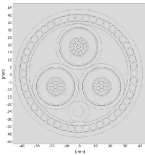
This study considers a 20 kV XLPE insulated power cable containing three copper conductors, each with a cross section of 95 mm² and having each a copper screen, as shown in

Fig. 1 Cross section of the considered three-phase export cable as modelled under COMSOL

Fig. 1. The sheaths are made of polyethylene and the bedding of polypropylene yarn. The surrounding armour is made of galvanized steel. This cable is currently installed in the SEM-REV test site located off Le Croisic, France and managed by Ecole Centrale de Nantes. Usual values regarding the cable material thermal properties, as provided in IEC standard 60853-2 [15], are presented in Table I.

TABLEI

CABLEMATERIALPROPERTIES

Layer Material Thermal conductivity [W.K-1_.m-1_] Volumetric heat capacity [MJ.m-3 K-1 ]

Conductor Copper (Cu) 370.4 3.45 Internal screen Semiconducting polymer 0.5 2.4 Insulation Cross-linked polyethylene (XLPE) 0.28 2.4 External screen Semiconducting polymer 0.5 2.4 Screen Copper wires (Cu) 370.4 3.45 Core sheath Polyethylene (PE) 0.2 1.7 Inner sheath Polyethylene (PE) 0.2 1.7 External

sheath Polyethylene (PE) 0.2 1.7 Armour Galvanized steel

wires 18 3.8 Filler Polyethylene (PE) 0.2 1.7

The static current carrying capacity of the considered cable is equal to 290A and is calculated according to IEC standards 60287-1-1 [16] and 60287-2-1 [17]. It is based on the following assumptions:

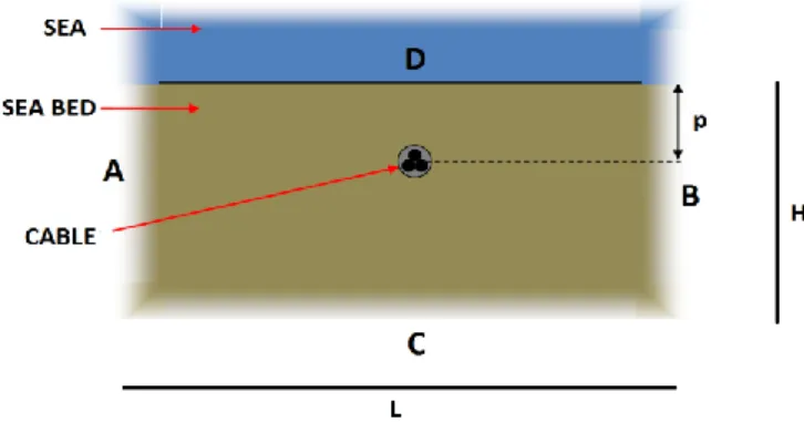
Fig. 2 Illustration of the cable environment and of its boundary conditions. - Maximal allowed conductor temperature at continuous

current load : 90°C - Current frequency : 50 Hz - Ambient temperature : 12°C - Cable burial depth : 1.5 m

- Thermal resistivity of surroundings: 0.7 K.m/W

B. Thermal Model

This section describes the development of a 2D finite element analysis (FEA) of the submarine cable thermal model using commercial software COMSOL. In order to predict the temperature distribution within the cable, the heat transfer equation of thermal conduction in transient state is applied [18]:

( )

where ρ is the mass density (kg.m-3), is the specific heat capacity (J.kg-1.K-1), T is the cable absolute temperature (K),

K is the thermal conductivity (W.m-1.K-1) and Q is a heat source (W.m-3).

The heat sources in cable installations can be divided into two generic groups: heat generated in conductors and heat generated in insulators. The losses in metallic elements are the most significant losses in a cable. They are caused by Joule losses due to impressed currents, circulating currents or induced currents (also referred to as “eddy currents”).

The heat produced by the cable metallic components (namely conductors, sheath and armour) can be calculated based on equations provided in IEC standard 60287-1-1 [16]. First, the Joule losses Wc of the conductor can be calculated by using the following formula:

( ( )) ( )

where R20°C is the resistance of the cable conductor at 20°C (W/km), α is the constant mass temperature coefficient at 20°C (K-1), and Ic (A) is the current density. Terms yp and ys are the skin effect factor and the proximity factor respectively. The sheath and armour losses (Ws and Wa respectively) can be calculated such as:

Fig. 3 Wave farm electrical network model as developed under PowerFactory λ

λ

where λ1 and λ2 are dissipation factors in the sheath and in the armour respectively. Insulating materials also produce heat. Dielectric losses in the insulation are given by:

where U0 is the applied voltage, δ is the loss angle, and ω is the angular frequency. However, the heat produced in the insulating layers expected to be significant, compared to the heat produced by the metallic components, under certain high voltage conditions only. Finally, the boundary conditions for this model are illustrated in Fig. 2. The modelled region is 7 m deep (H=7 m). The two side boundaries A and B are placed sufficiently far away from the cable so that there is no appreciable change in temperature with distance in the x-direction close to the boundaries. The cable is placed in the middle of the modelled region with respect to the x-direction, and its length is equal to 10 m (this value was proved sufficient in [19] for meeting the zero heat flux boundary conditions for sides A and B).

The soil surface C is assumed to be at constant ambient temperature of 12 ºC. The vertical sides A and B of the model are assumed to have a zero net heat flux across them due to their distance from the heat source. The equation in the side A and B is defined as:

( )

where n is the unit vector normal to the surface. On side D, the thermal exchanges via convection between the sea bed and the seawater must be taken into account. The heat convection exchange is defined as:

( ) ( )

where h is the heat transfer coefficient, Tout is the sea temperature and T the temperature of the upper boundary of the sea bed (side D).

C. Current temporal profiles injected in the cable

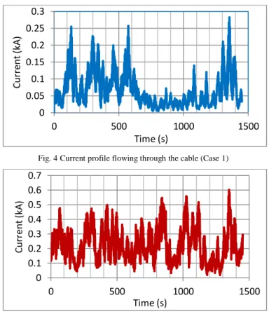
The wave farm is composed of 15 to 20 identical heaving buoys controlled passively and described in another paper [20]. Different power output temporal profiles for a single WEC were computed by means of several combined simulation programmes described in [21]. The first programme computes the wave excitation force at a single location in the wave farm. Then, the temporal profile of the excitation force is injected into a wave device model to obtain the corresponding electrical power output profile from which the wave farm power output is calculated. In order to model the device aggregation effect, the power output profiles of the other WECs composing the farm are computed by shifting the power profile of a single device by a random time delay, as described in a paper mentioned earlier [21]. These power profiles are then injected into an electrical grid numerical model which is shown in Fig. 3. This model has been developed under the power system simulator PowerFactory [22] and is described in more detail in [21]. The components of the offshore grid are highlighted in [21]. It is composed of 15 to 20 WECs, of a 0.4/10 kV transformer, of a 6.5 km-long cable, and of a 10/20 kV transformer. The rest of the network is located onshore is shaded in blue in the figure. Four current temporal profiles were simulated for different sea-state characteristics (the significant wave height Hs and the peak

period Tp) and device numbers, as detailed in Table II. They

are shown in Fig. 4 to 7.

TABLEII SIMULATION SCENARIOS

Case Sea-state characteristics Device number

Hs (m) Tp (s)

1 3 9 15

2 6 9 15

3 6 9 20

4 6 9 25

III. NUMERICAL SOLUTION

A. Model validation under steady-state conditions

A steady-state load current equal to 290A (i.e. equal to the steady-state capacity of the considered cable) is used for the analysis. If the model is valid, the conductor temperature should remain below its maximum allowed limit which is equal to 90°C. Table III summarizes the calculation of the different heat sources needed to solve the heat transfer problem according to the equations given in IEC standard 60287-1-1 [16]. The same heat fluxes are used as source terms for the FEA model, which allows to compare the calculated temperature with the two methods.

Fig. 4 Current profile flowing through the cable (Case 1)

Fig. 5 Current profile flowing through the cable (Case 2)

Fig. 6 Current profile flowing through the cable (Case 3)

Fig. 7 Current profile flowing through the cable (Case 4) 0 0.05 0.1 0.15 0.2 0.25 0.3 0 500 1000 1500 C ur rent (kA ) Time (s) 0 0.1 0.2 0.3 0.4 0.5 0.6 0.7 0 500 1000 1500 C ur rent (kA ) Time (s) 0 0.2 0.4 0.6 0.8 0 500 1000 1500 C ur rent (kA ) Time (s) 0 0.2 0.4 0.6 0.8 1 0 500 1000 C ur rent (kA ) Time (s)

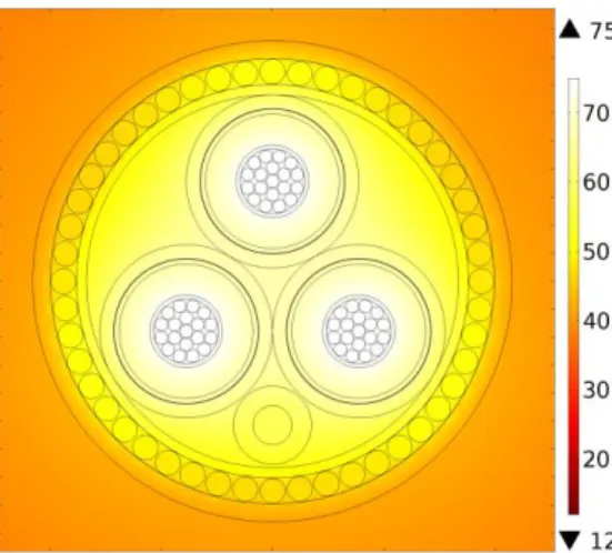
Fig. 8 Mesh model of the submarine cable as developed under COMSOL Fig. 8 shows the meshing of the submarine cable and its surrounding area that need finer elements because these areas are the most important sections of the presented analysis. Then, the areas which are far away from the cables can be modelled with a coarser mesh. The steady-state temperature field distributions in the cable and in its environment are shown in Fig. 9 and Fig. 10 respectively. The calculation from the IEC standard leads to a temperature of 67°C for the copper cores and 39°C for the external sheath. It can be seen that the maximum temperature of the copper conductor resulting from the FEA is 75°C while the external sheath reached 44°C, a little bit higher but in the same order of magnitude than the IEC standards. Note that both methods return copper core temperature below the critical temperature of 90°C, which provide a safety margin with a normal current load of 290 A. Despite the higher temperatures resulting from the FEA, one can see this results comparison as a form of validation of the model, especially considering that IEC standard uses a simplified model to calculate the temperature, i.e. an electric-equivalent circuit composed of thermal resistors and current sources. Hence, it leads us to conclude that the FEA model can be used to calculate the temperature of a submarine cable under fluctuating current as generated by a group of WECs.

B. Thermal response under a fluctuating current profile

This section describes the transient thermal response of the submarine cable to different current profiles as generated by an array of wave energy devices considering several sea states, as described in Table II. The objective of this study is to investigate the levels of current which can be transmitted through a submarine cable without the conductor exceeding the thermal limit of 90°C. For each simulated case, we consider the maximum value of the current and its percentage with respect to the continuous current rating of the cable, i.e. 290 A. Table IV shows that the maximum current of each current profile. It is important to highlight that these maximum currents can be far above the continuous current rating in all cases.

Fig. 9 Steady-state temperature field simulation (°C) of the submarine cable under normal load conditions.

Fig. 10 Steady-state temperature field simulation (°C) of the cable environment. The blue arrows represent the heat flux.

TABLEIII

HEAT LOSSES IN THE SUBMARINE CABLE

Losses type Formula

Numerical value (W/m)

Conductor Joule losses Wc 21.025

Sheath losses Ws 0.2

Armour losses Wa 0.027

Dielectric losses Wd 0.028

TABLEIV

CURRENT RESULTS FOR DIFFERENT SEA STATES AND DEVICE NUMBERS

Case Maximal current (A) Percentage of steady-state current rating (%)

1 283 97 2 602 207 3 4 709 833 245 287

Fig.11 Cable temperature versus time (Case 1)

Fig. 12 Cable temperature versus time (Case 2)

Simulation results of such a thermal problem depend on the initial conditions. Hence, it is important to accurately define the initial thermal conditions of the surrounding soil. The simplest initial condition which can be defined is a uniform temperature field. The value of this initial thermal condition should correspond to the case where the cable is subject to a current load equal to the average of the fluctuating current profile to be applied afterwards. The role of this first phase of the simulation is to quickly bring the cable temperature close to the expected range within which it is expected to vary once the fluctuating current profile is applied, thus reducing the simulation time. We used enough sequential repetitions of the current depicted in Figs 4 to 7 to reach a simulation time of 100 ks, i.e. a duration that is necessary to reach close-to-equilibrium conditions for the thermal problem.

Figs. 11, 12, 13 and 14 show the conductor thermal response versus time, for Cases 1 to 4 respectively. In these cases, the current maximal values are equal to 97% to 287% of the cable capacity. The maximum temperature does not exceed the allowed limit of 90°C for the first two cases. In other words, as the temperature is below the allowed limit of 90°C, the cable could be considered as overrated with respect to the considered current profiles. The third case presents good agreement between the sea state and the sizing of the cable (Fig. 13), as the temperature is close to the maximum allowed value of 90°C. Fig. 14 shows the simulation results for Case 4. In this case, the current maximal value is up to 287 % of the cable capacity but the temperature exceeds 90°C. Hence, the cable can be considered as underrated here.

Fig.13 Cable temperature versus time (Case 3)

Fig.14 Cable temperature versus time (Case 4)

In summary, under the conditions considered in this study, it appears that the cable is able to carry a fluctuating current profile whose maximum value is approximately equal to two and a half times the cable steady-state current rating.

CONCLUSIONS

This paper describes the results of a study focusing on the electrothermal response of a submarine cable to fluctuating current profiles as generated by a wave farm under different conditions, in particular regarding sea-state characteristics and the number of devices composing the farm. It was shown that the cable temperature remained below the allowed limit (equal to 90°C for the considered cable) when the maximum value of the injected current profile is as high as about two and a half times the (steady-state) rated current. Hence, it could be possible to size a cable to be included in a wave farm to the half of the maximum current, rather than to 100% of this current while keeping a good margin of safety. This could lead to significant savings in the CapEx of wave farm projects, thus contributing to improve the economic competitiveness of wave energy.

ACKNOWLEDGMENT

The research work presented in this paper was conducted in the frame of the EMODI project (ANR-14-CE05-0032) funded by the French National Agency of Research (ANR) which is gratefully acknowledged. This project is also supported by the S2E2 innovation centre (“pôle de compétitivité”). 16.5 17 17.5 18 95 96 97 98 99 100 Tem per at ur e (° C ) Time (x103 _s) 55 56 57 58 59 60 95 96 97 98 99 100 Tem per at ur e (° C ) Time (x103 _s) 82 84 86 88 90 95 96 97 98 99 100 Tem per at ur e (° C ) Time (x103 _s) 104 106 108 110 112 114 95 96 97 98 99 100 Tem per at ur e (° C ) Time (x103 _s)

REFERENCES

[1] Ocean Energy Forum. “Ocean Energy Strategic Roadmap 2016 - Building ocean energy for Europe”, 2016.

[2] E.ON “Wind Turbine Technology and Operations Factbook”, 2013. [3] S. Gasnier, V. Debusschere, S. Poullain, B. François, “Technical and

economic assessment tool for offshore wind generation connection scheme: Application to comparing 33 kV and 66 kV AC collector grids”, 18th European Conference on Power Electronics and

Applications (EPE'16 ECCE Europe), 2016.

[4] A. MacAskill, P. Mitchell, “Offshore wind—an overview”, Wiley

Interdisciplinary Reviews: Energy and Environment, Vol. 2, Issue 4,

2013.

[5] A. J. Nambiar et al. « Optimising power transmission options for marine energy converter farms”, International Journal of Marine

Energy, Vol. 15, pp. 127 – 139, 2016.

[6] C. Beels et al., “A methodology for production and cost assessment of a farm of wave energy converters”, Renewable Energy, Issue 12, Vol. 36, pp. 3402–3416, 2011.

[7] F. Sharkey, E. Bannon, M. Conlon, K. Gaughan, “Maximising value of electrical networks for wave energy converter arrays”, International

Journal of Marine Energy, Volume 1, April 2013, pp. 55-69.

[8] A. Blavette, D. O’Sullivan, T. Lewis, M. Egan, “Dimensioning the Equipment of a Wave Farm: Energy Storage and Cables”, IEEE

Transactions on Industrial Applications, Vol. 51, Issue 3, 2014.

[9] The Crown Estate, “Round 3 Offshore Wind Farm Connection Study”, version 1.0.

[10] R. Adapa and D. Douglass. “Dynamic thermal ratings: monitors and calculation methods”. Proc. of the IEEE Power Eng. Society Inaugural

Conf. and Exposition in Africa, p.163-167, 2005.

[11] J. Hosek. “Dynamic thermal rating of power transmission lines and renewable resource”, ES1002 : Workshop, March 22nd-23rd, 2011.

[12] Nexans, “Submarine cable 10kV, 6/10 (12)kV 3 core Copper XLPE cable, Cu-screen, Al/PE-sheath, Armouring”

[13] ABB, “XLPE Submarine Cable Systems Attachment to XLPE Land Cable Systems - User’s Guide”, rev. 5

[14] Nexans data sheet, technical reference: 2XS(FL)2YRAA RM 12/20 (24)kV, “3 core XLPE-insulated cables with PE sheath and armouring” [15] “Calculation of the Cyclic and Emergency Current Rating of Cables.

Part 2: Cyclic Rating of Cables Greater Than 18/30 (36) kV and Emergency Ratings for Cables of all Voltages”, IEC standard 60853-2, 1989.

[16] “Calculation of the current rating: Part 1-1 Current rating equations (100% load factor) and calculation of losses” IEC standard 60287-1-1, 2006.

[17] "Electric cables - Calculation of the current rating - Part 2-1: Calculation of Thermal Resistance”, IEC standard 60287-2-1, 2006. [18] C. Long. “Essential Heat Transfer. s.l”. : Longman 1 edition, 1999. [19] D. J. Swaffield, P. L. Lewin and S. J. Sutton, “Methods for rating

directly buried high voltage cable circuits,” in IET Generation,

Transmission and Distribution, vol. 2(3), pp. 393-401, 2008.

[20] T. Kovaltchouk, B. Multon, H. Ben Hamed, J. Aubry, F. Rongère, et

al., “Influence of control strategy on the global efficiency of a Direct

Wave Energy Converter with Electric Power Take-Off”, International

Conference and Exhibition on Ecological Vehicles and Renewable Energies (EVER), Monaco, 2013

[21] A. Blavette, T. Kovaltchouk, F. Rongère, B. Multon, H. Ben Ahmed “Influence of the wave dispersion phenomenon on the flicker generated by a wave farm”, EWTEC conference, Cork, Ireland, submitted. [22] DIgSILENT PowerFactory, http://www.digsilent.de/, accessed