In situ measurements of pH and O2 by planar optodes: improvements and adaptations for soil and rhizosphere applications

HAL Id: dumas-02893946

https://dumas.ccsd.cnrs.fr/dumas-02893946

HAL is a multi-disciplinary open access archive for the deposit and dissemination of sci-entific research documents, whether they are pub-lished or not. The documents may come from teaching and research institutions in France or abroad, or from public or private research centers.

L’archive ouverte pluridisciplinaire HAL, est destinée au dépôt et à la diffusion de documents scientifiques de niveau recherche, publiés ou non, émanant des établissements d’enseignement et de recherche français ou étrangers, des laboratoires publics ou privés.

improvements and adaptations for soil and rhizosphere

applications

Gabrielle Daudin

To cite this version:

Gabrielle Daudin. In situ measurements of pH and O2 by planar optodes: improvements and adapta-tions for soil and rhizosphere applicaadapta-tions. Inorganic chemistry. 2018. �dumas-02893946�

CONSERVATOIRE NATIONAL DES ARTS ET METIERS

PARIS

MEMOIRE

présenté en vue d’obtenir

le DIPLOME d’INGENIEUR CNAM

SPECIALITE : MESURE ANALYSE

OPTION : ANALYSE CHIMIQUE ET BIOANALYSE

par

DAUDIN Gabrielle

In situ measurements of pH and O

by planar optodes:

improvements and adaptations for soil and rhizosphere

applications

Soutenu le 4 octobre 2018

JURY

PRESIDENT : Christophe MOULIN (Professeur CNAM, Paris)

MEMBRES : Marie-Christine MOREL (Maitre de conférence CNAM, Paris) Chouki ZERROUKI (Maitre de conférence CNAM, Paris) Eva OBURGER (Dipl-Ing. Dr. BOKU, Vienne)

CONSERVATOIRE NATIONAL DES ARTS ET METIERS

PARIS

MEMOIRE

présenté en vue d’obtenir

le DIPLOME d’INGENIEUR CNAM

SPECIALITE : MESURE ANALYSE

OPTION : ANALYSE CHIMIQUE ET BIOANALYSE

par

DAUDIN Gabrielle

In situ measurements of pH and O

by planar optodes:

improvements and adaptations for soil and rhizosphere

applications

Soutenu le 4 octobre 2018

JURY

PRESIDENT : Christophe MOULIN (Professeur CNAM, Paris)

MEMBRES : Marie-Christine MOREL (Maitre de conférence CNAM, Paris) Chouki ZERROUKI (Maitre de conférence CNAM, Paris) Eva OBURGER (Dipl-Ing. Dr. BOKU, Vienne)

Acknowledgements

This manuscript is not just an assessment of 9 months of exciting internship. This work is the end point of 9 months of a great experience in Austria, in two research teams, and … almost 9 years of evening course at CNAM Montpellier and Paris. When I took this path, I didn't know where it would lead me. Today, I could not even say what pushed me to do such a long trip. It was a long trip, requiring a lot of perseverance, whereas during 4 hours, the course is only a succession of internet breaks..." Why? Why am I doing this?" And the next day, the motivation is still there. The CNAM is a school of perseverance, motivation, autonomy… It was a very rich professional and personal experience, sometimes challenging, always exciting. This adventure could not have succeeded without all the people who supported me, help me and believed in this project.

I would like to express my deep gratitude for Eva Oburger to welcome me within The Terrestrial Ecosystem Research group, University of Vienna, Vienna, and the Rhizosphere Ecology and Biogeochemistry group, BOKU, University of Natural Resources and Life Sciences, Tulln. It was really pleasant to work on her sides, between autonomy, trust and guidance. I learnt a lot during this internship! I would also thank warmly Hannès Schmidt, to welcome in his project and the pleasant collaboration during the first part of this internship. Thanks to them for giving me the opportunity to attend EGU 2017.

I would like to express my grateful thanks to Sergey Borisov, for providing prototypes, fluorescent probes, as well as for his expertise on the manufacture of optode and enlightening advice.

Of course, many thanks to Christina, without whom I could not have completed the experiments. And to your dad too... magic black box!!! No need to fix black curtains to windows anymore, and work in a black room, with a headlamp. Two intense months, but always in a good mood, even when the experiment were going wrong. I wish you every success for your PhD thesis.

I thank the colleagues of both teams, for their welcome, kindness and help. Especially to Daniel for his help for soil preparation and Veronika, always available and helpful. And also to Christoph, who kindly shared his knowledge about optodes and DGT. I also thank the students of the two labs, between barbecue evenings (even in winter!) and snowshoe expedition. Great time!

This course at CNAM and especially this internship would not have been possible without the support of Jean-Luc Chotte and Philippe Hinsinger. I would address my grateful thanks for allowing me to leave the team and do this internship. I particularly thank Philippe for proposing me to work on optode six years ago. It was completely new, and so, very exciting. Even if, we met a lot of setback, I got the virus, and I discovered the fascinating world of roots. Thanks a lot for having trusted me since the beginning of the EiCnam adventure, for

having followed my internship, taken time to answer my questions, and corrected this manuscript. It helped me to improve and progress during this internship. I thank INRA for having financially supported this course. Thanks to Farid and Candie for their essential administrative assistance. To all the Eco&Sols colleagues who supported me during all these years of CNAM, a big thank you! With a special thanks to Agnès and Claire, for your useful advices and warm talks. A special thought for Céline, and our optode team in Brazil… for sure optodes will go in-depth!

I also thank Marie-Christine Morel, for the help and support during the Paris step of the CNAM course, and for her constructive advice during the internship. The CNAM in Paris was not so easy, but the teaching by distance was most of the time very good. Thanks to all the analytical chemistry team.

Thank to my family for having always supported and encouraged me in this course and to my friends, for their support throughout this marathon. And finally, to the one who showed an unfailing support during this long road. Sometimes, you probably have wondered why I spent so many evenings in course and so many week-ends to study… It is a little bit crazy, isn't it? Yes, the CNAM is quite a venture!

I

Abbreviations

CCD Charge Coupled Device

CMOS Complementary Metal Oxide Semiconductor

DClFODA 2’,7’-dichloro-5(6)-N-octadecyl-carboxamidofluorescein DGT Diffusive Gradients in Thin film

DSLR Digital Single-Lens Reflex

FOCS Fiber-Optic Chemical Sensor

HO High pH Optode

HPTS 8-hydroxypyrene-1,3,6-trisulfonate

d-HPTS lipophilic 8-hydroxypyrene-1,3,6-trisulfonate

LA-ICP-MS Laser Ablation Inductively Coupled Plasma Mass Spectrometry

LED Light Emitting Diodes

LO Low-pH Optode

MWHC Maximum Water Holding Capacity

MY Macrolex Yellow

OxO Oxygen Optode

PBS Phosphate Buffered Saline

PtOEP Platinum (II)-octaethylporphyrin

PtTFPP Platinum (II)-tetra(pentafluorophenyl) porphyrin

RGB Red Green Blue

ROI Region Of Interest

ROL Radial Oxygen Loss

RSD Relative Standard Deviation

SD Standard Deviation

SE Standard Error

t-DLR time-domain Dual Lifetime Referencing

II

Figures index

Figure 1: Schemes of an optical and chemical sensor ... 5

Figure 2: Schematic representation of planar platform (A) and fiber-optic sensor (B). . .... 6

Figure 3: A typical Jablonski diagram ... 7

Figure 4: Schematic cross-section of planar optode ... 9

Figure 5: Bayer filter with Red, Green and Blue channels ... 11

Figure 6: Stern-Volmer plot. Theoretical (solid line) and incurved plot (dotted line). ... 13

Figure 7: Stern-Volmer plot affected by temperature. ... 14

Figure 8: pH sensor response in phosphate buffers with different ionic strengths. ... 16

Figure 9: Schematic representation of chemical processes occurring in the rhizosphere... 19

Figure 10: Rhizospheric boundaries regarding to chemical species: exudates accumulation, phosphate, nitrate and water depletion ... 20

Figure 11: Root-induced pH changes in Fe-deficient tobacco. ... 22

Figure 12: pH dynamics in Juncus effusus during 24h.. ... 23

Figure 13: pH spatio-temporal dynamic in the rhizosphere of chickpea and durum wheat in intercropping. ... 25

Figure 14: pH signal and soil cavities. pH map of chickpea and wheat rhizosphere (left). Picture of the corresponding rhizosphere area (right)... 26

Figure 15: pH optode application on Eucalyptus rhizosphere. (A) Pictures of Eucalyptus roots and applied optode. (B) Optode signal from roots. (C) Optode signal in homogeneous buffer solution afterwards. ... 28

Figure 16: Overview of development work ... 32

Figure 17: Planar optode scheme ... 34

Figure 18: Sensor layer coating ... 35

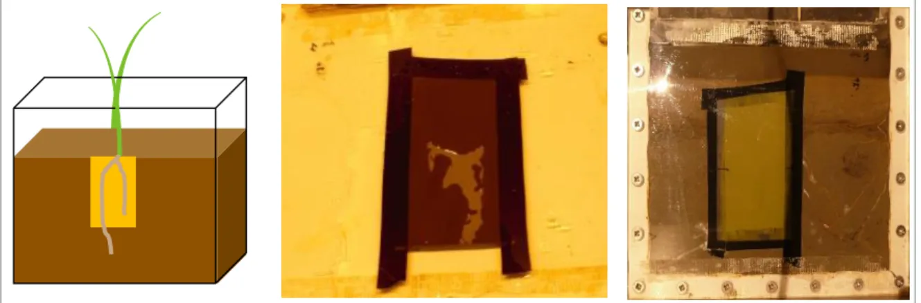
Figure 19: Rhizobox design with optode taped onto the removable front plate ... 38

Figure 20: Experimental set-up.(a) computer (b) excitation light device (c) Trigger led box (d) camera (e) rhizobox ... 39

Figure 21: Emission spectra of a typical oxygen sensor (Macrolew Yellow as reference dye and PtOEP as sensitive dye), at 100% of air saturation. Excitation wavelength = 445 nm. ... 41

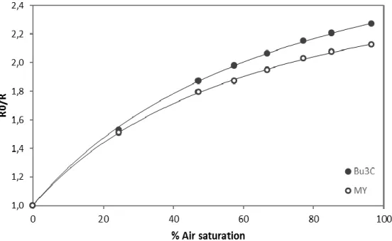
figure 22: Pixel intensity of the red and the green channel of Bu3C and MY optode ... 44

III Figure 24: Calibration curve of MY and Bu3 presented as the quenching efficiency

against oxygen content. ... 45 Figure 25: Image histogram. (A) Dark image. (B) Bright image. (C) Clipping image,

saturated. (D) Middle tones. ... 46 Figure 26: Optode construction with titan oxide. (a) With titan oxide extra layer (b)

Titan oxide embedded in the sensor layer ... 47 Figure 27: Pixel intensity of the Red and the Green channel of MY100 and MY300

optodes ... 48 Figure 28: Histogram of red picture in anoxic condition (0% air saturation). (a) Red

channel of MY100. (b) Red channel of MY300 ... 49 Figure 29: Calibration curve for MY100 and MY300 optodes. (A) presents Ratio value

against oxygen content. (B) presents quenching plot described by modified Stern-Volmer model (Eq.8) ... 50 Figure 30: Pixel value y from Red (A) and Green (B) channel of of PO-L, PO-MY1,

PO-MY3, PT-MY1 and PT-MY3. ... 52 Figure 31: Calibration curve of PO-L, PO-MY1, PO-MY3, PT-MY1 and PT-MY3. ... 53 Figure 32: Stern-Volmer plot of of PO-L, PO-MY1, PO-MY3, PT-MY1 and PT-MY3. ... 54 Figure 33 : Ksv and α parameters estimated from Stern-Volmer model of of L,

PO-MY1, PO-MY3, PT-MY1 and PT-MY3. ... 55 Figure 34: Emission spectra of LO (excitation wavelength = 445 nm) ... 56 Figure 35: Pixel intensity of Red (A) and Green (B) image of LO optodes at various

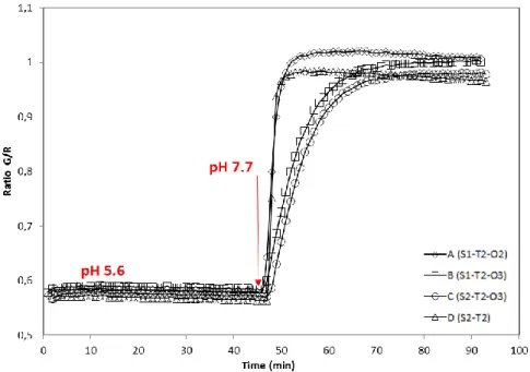
pH values.. ... 58 Figure 36: Calibration curve of optode A, B, C, D. ... 59 Figure 37: Response time curve. 45 min in phosphate buffer pH 5.6, then 45 min at pH

7.7. ... 60 Figure 38: Response time curve of optode E, without titanium oxide. ... 61 Figure 39: Emission spectra of HO. Excitation wavelength : 400 nm (A) and 445 nm

(B) ... 63 Figure 40: Pixel intensity of Green, Red and Blue image of HO, with pH changes ... 64 Figure 41: Calibration curve of HO. A, B, C represents ratio value of Green/Blue,

Red/Green, Red/Blue respectively. D is calibration curve with normalized ratio value.. ... 65 Figure 42: Image of foils stuck on the front plate screwed in the rhizobox filled with

flooded soil ... 69 Figure 43: Image of Ratio Red/Green of each oxygen optode ... 71

IV Figure 44: (A) Ratio R/G mean of water and soil area. (B) Drawing of water and soil

area ... 71

Figure 45: Calibration curve of optode NoC, Nyl, C0.5, C1, C2 and C10. (A) Calibration curve expressed from ratio Red/Green. (B) Stern-Volmer plot. ... 72

Figure 46: Standard deviation of ratio R/G values measured during the calibration. ... 73

Figure 47: Workflow of oxygen optode lifetime study ... 75

Figure 48: Stern-Volmer plot of NoC, Nylon, C0.5, C1, C2 and C10 optodes at Day 0 and Day 28. ... 76

Figure 49: Comparison of Ksv of model D-28 and model D-0. ... 77

Figure 50: Residuals of % air saturation estimation with model D-0 after 28 days. ... 77

Figure 51: Temporal variation of oxygen quenching efficiency Ksv ... 78

Figure 52: Picture of optode foil with carbon graphite spray layer, after 37 days in soils-water system. ... 79

Figure 53: Foils without sensor layer, applied to soil and root. ... 81

Figure 54: Response time curve. Ratio value of G/R for each LO. ... 82

Figure 55: Response time curve. Intensity pixel of Green (A) and Red (B) image. ... 83

Figure 56: Calibration curve of NoC, Nylon, C1 and C10 foil. ... 84

Figure 57: Background luminescence study. (A) Ratio G/R calculated picture. (B) Image of foil on soil-root system. ... 85

Figure 58: Ratio values of root and soil structures, extracted from ratio G/R picture with ImageJ by threshold. ... 85

Figure 59: Application of ratio Red / Green. (A) ratio image (B) graph of R/G ratio values of root and soil structures ... 87

Figure 60: Calibration curve of NoC, Nyl, C1 and C10 foil expressed from Red/Green Ratio ... 87

Figure 61: Drawing of rhizobox with soil and optode (upper diagram) and photograph of one rhizobox before measurement. ... 89

Figure 62: Time series of pH images of Exp I, from 5% to 76% of MHWC, and Exp II (88% and 97% of MHWC) ... 91

Figure 63: pH changes over time, for each water contact. (A) Exp I: 5% to 76% of MWHC. (B) Exp II 88% and 97% of MHWC. ... 92

Figure 64: Optode calibration procedure. (A) Calibration of optodes that are then directly used for measurements. (B) Calibration of small pieces of an optode foil with bigger pieces from the same foils used for measurement. .... 100

V Figure 65: Illustration of use of optode foil : a small piece for calibration and a big

part for measurement ... 102 Figure 66: Pictures of rhizobox with optode in place. ... 103 Figure 67: Calibration curve of optode A (Rhizobox 2) ... 104 Figure 68: Two-day imaging of oxygen concentrations in rhizosphere of rice (color

picture) and corresponding DLSR picture (gray scale). (A) Soil-water interface images (Rhizobox 2). (B) Rice rhizosphere images (rhizobox 1). ... 105 Figure 69: Illustration of oxygen concentration changes along root. ... 106 Figure 70: Illustration of spatio-temporal variation of oxygen concentration along

root tip. (A) Picture of root area in grey and corresponding oxygen map (in color) at day 1 and 2. (B) Graph of oxygen concentration changes with root growth. ... 107 Figure 71: Picture of a rhizobox with W shots and W powder in acidic soil. ... 109 Figure 72: Picture of rhizobox with tungsten input, nylon membrane and Low pH

optodes. ... 111 Figure 73: Calibration curve of LO optode at 5mM, 10mM and 45mM ionic strength. .. 112 Figure 74: Typical pH map for soil control (Bulk), W-shot and W powder. ... 113 Figure 75: Ratio, Green and Red images (pixels values) of LO optodes in buffer

solution used previously on W-powder. ... 114 Figure 76: pH profile of horizontal transect of LO (A) and pH map (B) ... 115 Figure 77: Calibration curve of oxygen optode made up with rutile <100 nm (rut) and

21 nm (21) titanium oxide. Up: Pixel values (mean) of green and red channels. Down: calibration curve expressed from ratio Red/Green. ... 127

VI

Table index

Table 1: Recipe of optode tested. ... 43

Table 2: Composition of optodes MY100 and MY 300 ... 48

Table 3: Details of optode recipe ... 51

Table 4: Thickness of each layer coated ... 57

Table 5: pKa’ of HO sensors. From normalized data (ratio at pH max = 1). SE = Standard error. ... 66

Table 6: Summarize of oxygen optodes prepared for optical insulation study. ... 70

Table 7: α and Ksv parameters describing Stern-Volmer model of optode NoC, Nyl, C0.5, C1, C2 and C10. ... 73

Table 8: Summary of foils tested for background luminescence study ... 80

Table 9: LO sensors prepared for calibration ... 81

Table 10: Boltzmann model parameters of NoC, Nylon, C1 and C10 optode. ... 84

Table 11: pKa’ value estimated from R/G and G/R calibration. ... 88

Table of contents

Abbreviations ... I Figures index ... II Table index ... VI

General introduction

1

Chapter I / State of the art and context

...

3

1. What is an optode? ... 5

1.1. Principles and generality ... 5

1.1.1. Definition ... 5

1.1.2. Sensing schemes of luminescence-based optode ... 6

1.1.3. Chemical part ... 9

1.1.4. Optical part ... 10

1.1.5. Application ... 11

1.2. Oxygen planar optode ... 12

1.2.1. Principles ... 12

1.2.2. Fluorescent oxygen probes ... 14

1.3. pH planar optode ... 16

1.3.1. Principle ... 16

1.3.2. Fluorescent pH probes ... 17

2. Soil and rhizosphere ... 18

2.1. Principles and generality ... 18

2.2. Measurement of biogeochemical processes in bulk and rhizosphere soil ... 20

2.2.1. Destructives approaches ... 20

2.2.2. Non destructives approaches ... 21

2.3. Planar optodes applied to soil and rhizosphere environment ... 23

Chapter II / Optode development

31

1. Experimental design ... 33

1.1. General experimental plan ... 33

1.2.1. Oxygen sensor preparation ... 35

1.2.2. pH sensor preparation ... 36

1.3. Optical instrumentation ... 37

1.4. Experimental procedures ... 38

2. Oxygen sensor (OxO) ... 40

2.1. Description and principles ... 40

2.2. Reference dye ... 43

2.3. Brightness enhancement ... 46

2.4. Sensitive dye ... 50

3. pH sensors ... 55

3.1. Low pH sensor (LO) ... 55

3.1.1. Description and principles ... 55

3.1.2. Optode thickness ... 57

3.1.3. Titanium oxide ... 61

3.2. High pH sensor (HO) ... 62

3.2.1. Description and principles ... 62

3.2.2. Set-up study ... 62

4. Adaptation for soil application ... 66

4.1. Soil-root system application: constraints ... 66

4.2. Oxygen optode ... 68

4.2.1. Optical insulation ... 69

4.2.2. Lifetime in flooded soils ... 74

4.3. pH optode ... 79

4.3.1. Optical insulation ... 79

4.3.2. Soil water content ... 89

5. Optode development: conclusion ... 93

Chapter III / Application projects

...

97

1. Imaging oxygen in rice rhizosphere ... 99

1.1. Context ... 99

1.2. Material and methods ... 99

1.2.1. Soil and plant conditions ... 99

1.2.3. Optode calibration ... 100 1.2.4. Rhizobox experiment ... 101 1.2.5. Oxygen imaging ... 102 1.3. Results ... 103 1.3.1. Optode calibration ... 103 1.3.2. Oxygen imaging ... 104 1.4. Conclusion ... 107

2. Imaging soil pH around tungsten input ... 108

2.1. Project overview ... 108

2.2. Material and methods ... 109

2.2.1. Soil and rhizobox preparation ... 109

2.2.2. Optode preparation ... 110 2.2.3. Optode calibration ... 110 2.2.4. Soil pH imaging ... 110 2.3. Results ... 111 2.3.1. Optode calibration ... 111 2.3.2. Soil pH imaging ... 112 2.4. Conclusion ... 116

General conclusion ... 117

APPENDIX 1 / EGU 2017 – Abstract ... 123

APPENDIX 2 / Titanium oxide supplementary test: comparison of different products 125 APPENDIX 3 / Protocol: preparation of oxygen optode ... 129

APPENDIX 4 / Protocol: preparation of Low pH optode (pH range: 5.5 – 7.5) ... 131

APPENDIX 5 / Protocol: preparation of High pH optode (pH range: 6.5 – 9.5) ... 133

1

General introduction

Soil is a highly complex matrix at the interface between atmosphere, biosphere, lithosphere and hydrosphere. It is a natural resource essential for sustaining human societies as it plays a central role in providing food, clean water and clean air. In soil, complex biogeochemical interactions drive key ecosystem functions such as plant productivity, regulation of greenhouse gas emissions, filtering and buffering of nutrients and contaminants [1]. Soil physical, chemical and biological heterogeneities induce spatial and temporal variabilities from the nanometre scale to the landscape scale [2]. Elucidating theses spatial and temporal dynamics at a fine scale is essential to better understand the interaction between inorganic and organic particles, roots, fungi and microorganisms in soil. However, accurate investigations of these dynamics require non-invasive approaches at the microscale avoiding disturbance of soil processes.

Planar optodes combine advantages of non-invasive and reversible methods. Based on the reversible changes of luminescence properties of a fluorescent probe, it allows the imaging of pH, O2 and CO2 at sub-mm scale, at high spatial and temporal resolution. Two decades

ago, planar optodes were first applied in marine sediment to monitor oxygen gradients at the water-sediment interface in situ [3]. Ten years later, planar optodes were first applied to image spatio-temporal pH dynamics in rhizosphere of plant species growing under waterlogged conditions [4]. This has opened new possibilities to obtain information of pH and O2 gradients in soil systems in a non-invasive way and to study rhizosphere processes

at the microscale. Oxygen and pH constitute the main parameters reflecting biogeochemical activities in soil, especially interactions between roots and soil [5]. Nonetheless, planar optode application in soil is still challenging. Soil is a highly heterogeneous system with complex physical and chemical properties. Optodes therefore have to be adapted to the specific environmental conditions [6].

This work presents the development and adaptation of oxygen and pH optodes for application in soil environments. In addition to the extensive developmental work, two distinct soil application studies were carried out. In the first one, oxygen dynamics in the rhizosphere of paddy field rice were monitored to reveal oxygen hotspots due to a radial loss of oxygen around roots in anoxic environment. In the second soil application study, pH optodes suitable for both, neutral and alkaline pH range, were applied to assess pH changes

2

around metallic tungsten sources in soils. The heavy metal tungsten is considered a green alternative to lead, however, little is known about the pH dependent solubility and therefore bioavailability of tungsten in soil environments.

The objectives were therefore (1) to design reliable optodes recipes to monitor oxygen and pH gradients in soil that are applicable in a laboratory not specialized in sensor chemistry, (2) to adapt optode construction and deployment for specific soil as well as soil-root interface applications, (3) to conduct two case studies using the improved planar optode setups. Development and application work was conducted in the laboratories of two research groups in Austria 40 km apart: The Terrestrial Ecosystem Research group, University of Vienna, Vienna, and the Rhizosphere Ecology and Biogeochemistry group, BOKU, University of Natural Resources and Life Sciences, Tulln. The work related to oxygen optodes was carried out mostly in Vienna, whereas development and application of pH optodes were done in the laboratories in Tulln.

The manuscript is divided in three chapters. Chapter 1 will be dedicated to a description of optode technology, focusing on oxygen and pH planar optodes. It will also present the scientific context of optode application in soils. Furthermore, it will include a critical overview of the current state of the art of optode applications in soil, addressing potentials, limitations and possible improvements. General information about important soil biogeochemical processes will also be presented. Chapter 2 will focus on the practical work, describing the conducted oxygen and pH optode development process followed by specific adaptations for soil and rhizosphere applications. Finally, the third chapter will present the two application projects

3

Chapter I

5 1. What is an optode?

1.1. Principles and generality 1.1.1. Definition

An optode (from the greek optós visible or optical and odós way) is an optical and chemical sensor. As defined by Cambridge [7], a chemical sensor is “a miniaturized analytical device

which can deliver real-time, online information on the presence of specific compounds or ions in complex samples”. Optodes have been developed since 1980s with the emergence of

opto-electronics devices, such as low-cost miniaturized light sources and high quality fiber-optics, as it met the needs of biomedical and industrial of real-time and continuous monitoring. An optode can be describe as two connected platforms: (1) the sensing platform or transducer, in contact with the analyte of interest and (2) the signal processing platform that detects and recordsthe optical signal related to the analyte concentration. Figure1features the schemes of an optode. The sensing platform is the chemical part of the sensor. It interacts with the analyte of interest by changing the optical properties of the sensors. Then, the signal processing platform records the change of optical properties.

Most optical chemical sensors are based on changes of absorption and fluorescence properties [6]. The optical sensing platforms include optical fibers and planar platforms that record and transduce optical signals emitted by the chemical sensor into data related to the concentration of analyte. Fiber-optics and planar platforms differ by their geometry and the format of output data. Fiber-optic records signal from the chemical sensor in one point whereas planar platform gives a data matrix with a spatial dimension (Figure 2). Consequently, fiber-optic can be defined as a 1-D optical platform and planar platform as a 2-D one. Optode sensors using planar platform are called planar optode and are associated with an imaging optical system.

Chapter I / State of the art and context

6

One typical fiber-optic chemical sensor (FOCS) is a doped cladding system with the coating of the chemical sensing platform at the tip. Contrast to the planar platforms, it cannot be used for non-invasive measurement as the chemical sensing part is integrated to the optical platform. These widely used FOCS are beyond the scope of this document, as we focus on 2-D optical platform giving a spatial information.

Optodes have numerous advantages. They are easy to handle and often reach higher sensitivity than electrochemical sensors. Moreover, remote systems allow non-invasive and multi-analyte measurements [8].

While optical chemical sensor is a very wide topic, this review will focus on planar optode based on fluorescence transduction and summarize the principles of luminescence-based optode (sensing schemes), optical platforms and the chemical part of the optode. Analytes of interest and application areas will also be presented.

1.1.2. Sensing schemes of luminescence-based optode

Luminescence based optodes use the change in optical properties of a luminescent probe when interacting with the analyte of interest. Luminescence is the light emission of a molecule occurring from excited states due to photon absorption [9]. This process is described by the Jablonski diagram, as presented in Figure 3. When absorbing light, a fluorophore, in electronically fundamental state S0,is excited to a higher electronic state S1 or S2. A fluorophore

in S2 state relaxes quickly to the excited state S1 by internal conversion. Then, to return to the

ground state S0, the fluorophore can follow two ways. The first one is de-excitation by light

Figure 2: Schematic representation of planar platform (A) and fiber-optic sensor (B). (Adapted from Wencel, 2014 [6]).

7

emission, called fluorescence. The relaxation occurs in the nanosecond range. The second one is the intersystem crossing with a conversion from the singlet state S1 to a triplet electronic state

T1. Then, there is relaxation to the ground state S0 by light emission called phosphorescence

occurring at a longer time (millisecond).

Luminescence properties of a probe can be described by two parameters: luminescence intensity and decay-time of luminescence. The choice of the parameters will define the chemical construction of the optode as well as the optical sensing platform.

o Fluorescence intensity

The measure of fluorescence intensity under continuous light-excitation is the easiest method to perform optode measurements. However, fluorescence intensity is not only dependent on the concentration of the fluorophore as described by Parker’s law:

𝐼 = 𝐼0 . 𝜀 . 𝐶. 𝑙. 𝑄. 𝑘 (1)

Where 𝑰 is the intensity of luminescence, 𝑰_𝟎 the intensity of the light source, 𝜺 the molar absorption coefficient (L.mol-1.cm-1), 𝑪 the concentration of fluorophore (mol.L-1_{), 𝒍 the length}

of the penetrated layer or thickness (cm), 𝑸 the quantum yield of the fluorophore and 𝒌 a coefficient related to the geometry of the optical set-up.

Fluorescence intensity is also affected by the disturbance of the light source, ambient light, inhomogeneity of probe distribution and thickness of the sensor, as well as background luminescence. Also, leaching of the probe or photobleaching will decrease the fluorescence

Chapter I / State of the art and context

8

intensity. Two methods can overcome these critical drawbacks of fluorescence intensity measurement: (1) Time-resolved fluorescence, (2) Ratiometric measurements [10].

Time resolved fluorimetry is the measurement of the fluorescence intensity at a certain time interval after excitation by a short light pulse. This method can only be applied with a long-decay time probe. It enables to background fluorescent to be suppressed (in the case of short-decay time signal), but does not eliminates heterogeneity of excitation light, artefacts from ambient light, probes inhomogeneity or probes leaching [8].

Ratiometric approach is more widely used and based on the fluorescence intensity measurement at dual excitation wavelengths and/or dual emission wavelengths. Two approaches can be used. The first approach relies on the excitation and/or emission wavelength shift when the sensitive dye reacts with the analyte. For example, 8-hydroxypyrene-1,3,6-trisulfonate (HPTS) pH sensitive probe exhibits a pH-dependent shift of its absorption band. As result, HPTS excitation spectra present two separated fluorescence peaks at 428 nm and 505 nm for the acidic and basic form of HPTS. The ratiometric approach can thus be applied by measuring the fluorescence emission at 540 nm at both excitation wavelength [11]. The second approach consist of combining an inert fluorophore with the sensitive probe and measure fluorescence intensity of both probes. The fluorescence of the inert fluorophore acts as reference signal. To provide sufficient signal sensitivity, the sensitive and non-sensitive dye have to present a sufficient Stokes shift to discriminate reference signal from analyte dependent signal. The ratiometric approach overcomes some disadvantages of intensity measurement, such as the drift of the light source, sensor thickness heterogeneity or inhomogeneity of the fluorophore distribution in the sensor layer (to some extent). Combination of two probes might be prone to drifts due to photobleaching or probe leaching as both probes may have different physical and chemical properties. The intensity ratiometric approach is mainly combined with an imaging sensing platform, particularly, the combination of sensitive and non-sensitive dyes combined with digital camera as reported for few years [12].

o Fluorescence decay time

The decay time or lifetime of a fluorescent probe is unique and independent on wavelength emission. It is defined as the time available for a fluorophore to get information about its

9

emission, or the time to decay from the excited state S1 to the ground state S0 with light emission

[9]. Fluorescence lifetime-based measurement aims to record lifetime of excited state of the fluorophore after a short pulse of light. This approach is classified by two domains: the time-domain and the frequency-time-domain [9].

Lifetime measurement is superior to intensity measurement as it is not affected by the concentration of fluorophore and it is independent of wavelength dependant interferences [13]. However, it requires a highly sensitive and fast gateable optical set-up to record signals in the 10-6s time range. Optical set-ups are fiber-optic or expensive CCD (Charge Coupled Device) camera.

To overcome the complexity of lifetime measurement, especially with short decay time fluorophore, a referenced time domain method was developed by Liebsch, called time-domain Dual Lifetime Referencing (t-DLR) [13]. A short-lived sensitive probe and a long-lived reference probe are excited by a short pulse of light. Images are taken at two different times: the first one during the short pulse, the second when the excitation light is off. The first image records intensity from the sensitive probe and the reference probe. The second image records the signal during the decay time of the long-lived reference probe.

1.1.3. Chemical part

The sensing platform is built of three parts: the support layer, the sensor layer and a supplementary layer as described in the Figure 4.

The support layer is designed to make the optode easy to handle. It has to be optically transparent, chemically compatible and inert with the sensor layer. The most common support material is transparent polyester foil [12]. It also possible to use glass or Perspex support [14], or even to spray sensor directly on to the sample surface [15].

The sensor layer, coated onto the support layer, is made of a matrix containing fluorescent probes. Matrix serves as a physical support for the probes immobilization, prevents it from

Chapter I / State of the art and context

10

diffusion into the measurement environment and helps to achieve a homogenous distribution of the probes. Also, matrix properties play an important role for the diffusion of the analyte towards the probes and therefore can define the sensitivity of the sensor [16]. The most common material is a polymer class matrix covering among others, like polystyrene [17] and polyvinyl-alcohol [18], cellulose acetate [19], ethyl cellulose [20] and hydrogels (e.g. polyurethane) [21]. Recently, sol-gel based materials were also introduced as they present better optical transparency and can be tuned for specific chemical and physical properties [22]. Fluorescent probes are immobilized in the matrix in three mains ways: adsorption, covalent binding and entrapment. Adsorption method is the least reliable as the probe can easily leach out. Covalent binding is a complex process, time consuming and needs appropriate materials. This method is very reliable and eliminates probes leaching issues. However, covalent binding may cause a change of optical properties of the dye and therefore reduce the sensor performance [6]. Entrapment is the easiest one and it is a fast method. It is also the method used most widely, especially for teams that do not specialize in sensor chemistry. However, slow leaching of probes can occur over time. Additives can also be included in the sensor matrix to improve performance of the sensor. A typical one is scattering particles as SiO2 and TiO2 to enhance

excitation efficiency by a multiple light scattering in the sensor layer [23].

On top of the sensor layer, a supplementary layer can be coated to protect from interfering sample fluorescence. This layer act as an optical insulation. It has to be permeable to the analyte and requires good adhesion properties to the sensor layer. Optical insulation may result in an increase of the sensor time response due to a longer path between the sample and the probe immobilized in the matrix. Polymer layers such as hydrogel in which carbon black is entrapped and coated on to the sensor layer are most frequently used as supplementary layer [24]. White membranes applied between the optode and the sample were also reported [25].

1.1.4. Optical part

The signal processing platform aims to measure luminescence properties emitted by the sensing part. It requires a light source and a photodetector that records light emitted by the optode. Excitation light is delivered by a light source such as Xenon lamps [18] or LEDs (light emitting diodes) [21]. As LEDs are low-cost light source and exhibit interesting spectral properties with narrow spectral band, they are more currently encountered in optode measurement set-ups.

11

Photodetectors record light emitted by the sensor. In the case of planar optodes, imaging set-up use CCD (Charge Coupled Device) or CMOS (Complementary Metal Oxide Semiconductor) cameras. Lifetime measurements are performed with high expensive CCD cameras as they require a very fast shutter to be able to record signal at a short time interval [13]. CMOS cameras are preferred for intensity measurement. Recently, low-cost imaging system has appeared with commercial digital DSLR (Digital Single-Lens Reflex) cameras [18]. These colour cameras provide red, green and blue signals for each pixel (RGB approach) due to its Bayer filters (Figure 5). Depending on spectral properties of fluorophore probes, each individual channel can be used for ratiometric measurements. Thus, it is possible to combine up to three indicators with discriminated emission wavelengths allowing a dual sensing [26].

It has been shown that the RGB approach presented a reduced spatial standard deviation and a higher signal-to-noise ratio compared to black/white CCD camera [27]. CMOS camera is therefore an affordable system (<1000€), very easy to handle, portable, and can be used with or without optical filters. However, digital cameras do not protect from excitation light inhomogeneity or dye photobleaching. Even if lifetime measurements by CCD cameras represent the most accurate system with the best spatial homogeneity, the RGB approach provides a good compromise between robustness and cost. It will therefore be used for the experimental work. Therefore, hue parameter (tint) of DSLR color camera can also be exploited for imaging approach with a better quantification that ratiometric intensity RGB approach as recently reported [28].

1.1.5. Application

Planar optodes are used in a wide range of applications. The first environmental/ecological optode application was carried out on marine sediments to study oxygen profiles at the

Chapter I / State of the art and context

12

sediment interface [3]. Since then, numerous studies have been published reporting spatial and temporal dynamics of oxygen and pH profiles in sediments [11,18,29]. Another current application in sediment is the imaging of oxygen in the rhizosphere of plants grown under waterlogged conditions (e.g. paddy field rice) as these plants develop strategies to withstand the anoxic environment and toxic elements [30]. During the past decade, planar optode have been applied to investigate rhizosphere processes in soil under both upland (aerobic) and paddy field (anaerobic) conditions by imaging of O2, pH and CO2 gradients around roots from

different plant species, like chickpea and wheat and rice [31,32,33]. More recently, optodes were also used in soil to study the impact of oxygen on N2O emissions in soils amended with

manure [34]. Finally, planar optodes are also used for bioprocess monitoring [25] and even in medical application to follow in vivo wound healing [35].

In terms of target analyte, most of optodes are dedicated to oxygen and pH imaging as cited above. Then CO2 optodes were developed [36]. Other analytes were also explored, like nitrate

[37], ammonium [38], ammonia [39], hydrogen sulfide [40], potassium [41]. Optodes can also be applied to monitor physical parameter as temperature [42] or pressure [10]. An optode was also developed to monitor the enzymatic activity of leucine-aminopeptidase [43]. Finally, some optodes were developed for multi-sensing such pH and O2 dual sensing [44] and even a

multilayer optode for simultaneous imaging of O2, CO2, pH and temperature [42].

1.2. Oxygen planar optode 1.2.1. Principles

Oxygen optodes are based on the ability of oxygen to quench the fluorescence of many dyes [45]. The oxygen quenching responds to the model of dynamic quenching due to the collision between oxygen and the fluophore. It is described by the Stern-Volmer equation [9]:

(2)

Where, 𝑰_𝟎 and 𝑰 are the fluorescence intensities in the absence and presence of quencher respectively; 𝒌𝒒 is the bimolecular quenching constant; 𝝉𝟎 is the lifetime of the fluorophore in

absence of quencher, and [Q] is the concentration of quencher. 𝐼0

13

The Stern-Volmer quenching constant is given by:

(3)

𝑲_𝒔𝒗 is generally related to the overall quenching efficiency of the oxygen probe. The quenching plot or Stern-Volmer plot is often represented by the ratio 𝐼0

𝐼 in function of [Q]. In theory, this

plot should be linear. Thus, K_𝑠𝑣−1 is the concentration of the quencher when half of 𝐼₀ is lost. The bimolecular quenching constant 𝑘_𝑞 reflects the efficiency of the quenching or in other words the accessibility of the fluorophores to the quenchers. Also, as 𝜏₀ influences Ksv constant,

a probe with a long-lived excited state lifetime is a more efficient fluorescence quencher. In an optode, the probe is entrapped in a matrix reducing probe accessibility to oxygen. The Stern-Volmer plot of an oxygen optode is not linear and is incurved towards x axis (Figure 6).

It is generally described by a modified Stern-Volmer equation [46]:

(4)

Where 𝑰𝟎 and 𝑰 are the fluorescence intensities in the absence and presence of quencher

respectively, 𝑲𝒔𝒗 is the overall quenching constant, 𝜶 is the fraction of fluorescence of the

probe which is not quenched significantly by oxygen. 𝐼₀ 𝐼 = (_{1 + 𝐾}1 − 𝛼 𝑠𝑣 . [𝑂2] + 𝛼) −1 𝐾_𝑠𝑣 = 𝑘_𝑞 . 𝜏₀

I

/I

[Q]

Figure 6: Stern-Volmer plot. Theoretical (solid line) and incurved plot (dotted line).

Chapter I / State of the art and context

14

Finally, as the collisional quenching is affected by temperature (Figure 7), oxygen optode measurement are cross-sensitive to temperature [47]. It means that oxygen measurements with optodes should be carried out at constant temperature or results have to be corrected.

1.2.2. Fluorescent oxygen probes

Oxygen fluorescent probes available are numerous and grouped into several chemical classes. As the subject is very wide and well documented, I will present it briefly and focus especially on dyes most commonly used.

The two main classes of oxygen probes are (i) organic probes and (ii) metal-ligand complexes. Organic probes include polycyclic aromatic hydrocarbons (PAHs) and fullerene. Pyrene based PAH probes are considered as the first generation of oxygen probes [23]. They present a strong luminescence and a good photostability. Fullerene based probes possess also interesting chemical properties like a large conjugate structure resulting in a high sensitivity for oxygen. For example, fullerene C70 was used as for oxygen trace sensor in the ppbv range [48].

The second main class are metal-ligand complexes which are nowadays most commonly used in oxygen sensors. It is a wide class of probes with useful properties such as relatively long lifetime, absorption band in the visible and a large Stokes shift. This class of probes contains transition metal complexes such as ruthenium and iridium complexes, and the large group of porphyrins and metalloporphyrines. Ruthenium complexes, especially ruthenium(II)-tris-4,7-diphenyl-1,10-phenantroline (Ru-ddp) have been widely used as it possesses long-lived emission, from micro-second to millisecond. It has suitable properties for the decay time approach as described by Holst and Frederiksen who applied oxygen planar optodes based on

Figure 7: Stern-Volmer plot affected by temperature.

I

/I

[Q]

T°

15

Ru-ddp with lifetime measurement on the sediment-water interface [49], as well as on the rhizosphere of flooded plant species in sediment [50]. In contrast, iridium complexes possess a short response time, high sensitivity, higher brightness and they are less sensitive to temperature. For example, cyclomateleted iridium(III) coumarin complexe based oxygen sensors present an outstanding brightness and a low cross-sensitivity to temperature. Its spectral properties allow the application of both, the ratiometric or the decay time approach, but its photostability is poor and much lower than that of Ru-ddp [47].

The most frequently used oxygen probes are metalloporphyrin complexes with platinum or palladium. These probes show strong absorption and a high quenching efficiency. Among the large group of metalloporphyrins, fluorinated ones such as platinum(II)- tetra(pentafluorophenyl) porphyrin (PtTFPP) and the non-fluorinated, platinum(II)-octaethylporphirin (PtOEP) are most common [23]. Both have an absorption band in the visible and present a large Stokes shift. PtTFPP is more photostable than PtOEP. It was used during several months in sediments without major shifts [51]. However, PtOEP is highly sensitive to low oxygen concentrations and preferred for oxygen depleted environments as showed by Oguri, with the highest sensitivity in the oxygen concentration range of 0-50 µmol.L-1 and a higher brightness than PtTFPP [17]. This study also revealed no shift of the signal during 19 hours of continuously light exposure.

As oxygen probes rely on long lived emission properties insuring high quenching efficiency, oxygen sensors are often combined with the fluorescence decay time approach. However, with the emergence of low cost imaging systems, and the large Stokes shift of some sensor, especially for metalloporphyrin, the ratiometric approach is also available. Larsen proposed an oxygen planar optode made up of PtOEP oxygen probes mixed with the non-sensitive probe Macrolex Yellow, entrapped in polystyrene matrix [12]. PtOEP emits in the red part of the spectrum whereas Macrolex Yellow emits in the green. Measurement are typically carried out with a RGB camera and results are reported based on ratiometric calculations between the intensity recorded by the red and green channel. This simple approach makes the method accessible to non-specialists with significantly lower cost than decay time measurement.

Chapter I / State of the art and context

16 1.3. pH planar optode

1.3.1. Principle

pH optode measurement is based on a difference in optical properties of protonated and deprotonated forms of a weak organic acid. A change of proton concentrations modifies the concentration ratio between acidic and basic form of the pH probe. The fluorescence intensity measured is correlated to this change of equilibrium between protonated and deprotonated form of the pH probes [52]. Thus, optical pH sensors measure the concentration ratio between acidic and basic form of the fluorophore. As for electrochemical pH sensors, pH changes follow the Henderson-Hasselbach equation:

(5)

Where 𝒑𝑲𝒂 is the negative logarithm of the acid dissociation constant, [𝑨] and [𝑨𝑯] are the concentration of acidic and basic form of the probes, 𝒇_𝑨 and 𝒇_𝑨𝑯 are the activity coefficient of the acidic and basic form of the probe.

As described by the equation (5), pH value is defined also in terms of activities, meaning that pH optodes are cross sensitive to ionic strength. Figure 8 presents the pH response of a pH sensor based on 8-hydroxy-1,3,6-pyrenetrisulfonic acid (HPTS) in buffer solution with different ionic strengths [18]. The interference varies with the charge of the fluorophore and the ionic strength of the environment.

𝑝𝐻 = 𝑝𝐾𝑎 + 𝑙𝑜𝑔 [𝐴]

[𝐴𝐻]+ 𝑙𝑜𝑔 𝑓_𝐴 𝑓_𝐴𝐻

Figure 8: pH sensor response in phosphate buffers with different ionic strengths. (From Zhu, 2005 [18])

17

Since the changes of fluorescence intensity with pH are described by a sigmoidal relationship, the dynamic pH range is limited to pKa ± 1.5 [6]. In addition, the pKa of the pH probes inserted in a matrix is different and will be called 𝒑𝑲𝒂′ in the manuscript. Thus, pH dynamic range of a probe can be tuned with the host matrix and methods of immobilization. For example, the pKa’ of pH probe 8-Hydroxy-1,3,6-pyrenetrisulfonic acid (HPTS) has found to be at 6.7 in ethyl-cellulose [20], 7.7 in Dowex resin [25], and 7.1 in polyvinyl alcohol [18].

1.3.2. Fluorescent pH probes

HPTS and its derivatives as well as fluorescein based probes are typical pH fluorophores with HPTS based probes being most widely used. It is a great choice for ratiometric approach, as its excitation spectra is pH dependant [11]. The ratiometric approach can be applied at dual excitation wavelength and single emission. Also, as explained above, its dynamic range can be changed with the matrix, from neutral range towards alkaline range. In addition, it exhibits a good photostability. However, HPTS presents high sensitivity to ionic strength [53]. Also, as it is very hydrophilic, HPTS can be chemically modified to render it more lipophilic [54]. Thus, modified HPTS can be entrapped in a matrix and not only covalently bound [12].

The main alternative to HPTS is fluorescein and its derivatives. In contrast to HPTS, it exhibits a low photostability. However, it is less sensitive to ionic strength [55]. A series of chlorofluorescein esters were designed that were lipophilic and can be entrapped in a hydrogel matrix. These fluorescein derivatives probes show a marginal shift of their pKa’ with ionic strength changes. Also, depending on the halide substituent added to the fluorescein ester base, the pKa varied from 5.5 to 7.3 allowing different pH dynamic ranges [55]. Moreover, these chlorofluorescein pH probes exhibited higher photostability than the fluorescein chromophore. Another lipophilic and low sensitive to ionic strength fluorescein derivative is carboxyamidofluorescein class designed for marine sediment application [21]. They also presented high quantum yield and pH dynamic range in the alkaline range, from 7.2 to 9.2. However, these probes showed poor stability in light exposure [56]. Finally, a commercial available fluorescein derivative, 5-hexadecanoylaminofluorescein, present also lipophile properties as well as low cross sensitivity to ionic strength. With a pKa’ in hydrogel at 6.6, this pH probe was used to study pH dynamics in rhizosphere of lupin combined with intensity based approach [57].

Chapter I / State of the art and context

18

Due to the sigmoid response of pH probes, the dynamic range is limited to 3 pH unit. In consequence, it is not possible to monitor pH across a wide range. This is only possible by mixing two pH probes in the matrix as presented by Weidgans [55]. Two lipophilic fluorescein esters were combined in hydrogel matrix with a dynamic range of pH 4.5 to pH 8.5. Also, a larger dynamic range was proposed by Schreml to investigate pH changes of wound healing in humans in situ [58]. Alternative to the combination of two probes, fluorescein-5-isothiocyanate (FITC) pH sensitive probe was covalently bound to aminocellulose particles and mixed to a reference dye in hydrogel matrix. It exhibited reliable pH measurement in a range of pH 3 to 9, and was suitable to detect inflammatory phase within wound healing.

The dynamic range of fluorescent pH probes is usually between 5 and 9. Optodes suitable for acidic environments below pH 5 are rare. One optode for a pH range between 2.5 to 4.5 was developed by PreSens GmbH [59]. In the extreme alkaline pH range, a recent publication described a planar optode for alkaline sediment based on chloro phenyl imino propenyl aniline (CPIPA) with a dynamic range from pH 7.5 to pH 10.5 and a negligible cross sensitivity to ionic strength if below 0.1 mol. L-1 [60].

2. Soil and rhizosphere

2.1. Principles and generality

Soil is a highly complex and heterogeneous living environment in the biosphere. It consists of a mineral and organic matrix (such as humus), as well as living organisms (microorganisms (bacteria, fungus) and fauna. This heterogeneous environment is the place of many interactions at fine scales with consequences on soil functioning at landscape scale. In particular, biogeochemical interactions at microscale are of abiotic and biotic origin. Abiotic processes include freezing/thawing as well as drying/wetting and they alter soil structures (aggregates and pores) and redox conditions. Biotic factors involve living roots and rhizodeposition, root turnover, litter fall, fauna activity (burrowing). This factors induced chemical and biological processes such as denitrification/nitrification or carbon mineralisation [61].

One of the main hotspot of biogeochemical activity is the rhizosphere. Defined as the amount of soil around living roots which is influenced by root activity [5], the rhizosphere is the place of intense interactions between soil particles and roots: water and nutrient absorption, anions

19

and cations exchange, release of organic and inorganic (H+_{, OH}-_{) molecules, and respiration.}

This exchange between roots and soil modifies the chemical equilibrium around roots potentially changing rhizosphere soil pH and redox conditions. Rhizosphere processes are highly dynamic, both at the temporal and spatial scale. Figure 9 summarizes the main biogeochemical processes in the rhizosphere [62].

Plant-soil interactions induce pH changes in the rhizosphere that affect the bioavaibility of nutrients and toxic elements. The flux of protons and hydroxyls between soil and roots is triggered by many interactions: balance of cation and anion exchange, release of organic root exudates and CO2 (respiration of roots and rhizosphere microorganisms), and is affected by

redox conditions, soil buffering capacity, nutritional constrains [63]. pH is thus of major ecological relevance in roots and soil functioning.

A particular important parameter is oxygen as redox conditions drive lot of chemical reaction in soil. In addition, oxygen is required by the plant for root cell respiration which is of major importance for wetland plant living in anoxic condition. In order to uphold root respiration under flooded conditions, plants developed aerenchyma tissue (gas channel) to transport oxygen from leaves to roots. This oxygen transferred to the rhizosphere by a phenomena called radial oxygen loss, additionally protects roots from toxic element that are highly soluble under reduced conditions (e.g. H2S) [64].

Figure 9: Schematic representation of chemical processes occurring in the rhizosphere. (From Hinsinger, 2005[60])

Chapter I / State of the art and context

20 2.2. Measurement of biogeochemical processes in bulk and rhizosphere soil

Biogeochemical heterogeneity in soils and rhizosphere can be measured by two approaches: destructive and no destructive.

2.2.1. Destructives approaches

Destructives approaches involve sampling of soils and analysis of target analyte after extraction steps. These approaches are subject to international standards such as pH, phosphate or organic carbon measurement in soils. However, these widely used methods have some disadvantages. Firstly, the sampling of particular soil compartments can be very challenging. Indeed, the separation of rhizosphere from bulk soil is highly challenging. As defined above, rhizosphere soil is the amount of soil subject to root-induced activity. However, this influence varies for different elements or parameters of interest [65]. For example, the phosphorus depletion zone around the root is about 3 mm while that of nitrate is about 2 cm as displayed in Figure 10.

From a practical point of view, it is common to define the rhizosphere soil as the soil adhering to the roots. However, the thickness of this soil layer is highly dependent on soil texture and moisture level, as well as root morphological properties which makes this sampling random and imprecise. Secondly, with sampling being destructive, a temporal analysis of the same plant/

Figure 10: Rhizospheric boundaries regarding to chemical species: exudates accumulation, phosphate, nitrate and water depletion (From York, 2016 [65])

21

rhizosphere spot is not possible. Destructive spatial analysis at the millimetre scale is also tricky since a sufficient amount of soil (mostly several gram) is needed to carry out the analyses.

2.2.2. Non destructives approaches

Non-destructive approaches aim to measure biogeochemical properties of soils in situ. Experimental approaches can be classified into two main categories: (1) invasive methods and (2) non-invasive methods.

The invasive methods include electrodes and microelectrodes, and optical microsensors. Electrodes are based on electrochemical principles and are specific to a target analyte. They are mainly used for pH, gas such as N2O, CO2, H2S et O2, and ions (e.g. NH4+, NO3-).

Microelectrodes, with a small sensor tip (micrometer scale) have the advantages to allow high spatial measurement with a fast response [66]. However, these tools present some limitations in soils application as the sensor tip can be polluted by organic matter and soil components meaning a drift of the signal overtime. They can also consume a significant amounts of the target analyte. The optical microsensor, also called micro-optode, are based on optical fibers with a luminophore coated at the end tip. They present a fast response time (range of second), a long-term stability, does not consume target analyte and less fragile than microelectrodes. They are mainly used to monitore O2, H2S, H2, N2O, NO, pH and redox potential [66].

Even if microsensors allow in situ measurements over time, the procedure remains invasive and disturbing for the root-soil system. Also, spatial monitoring along roots requires the insertion of many microsensors in the study area. An alternative is the implementation of non-invasive methods providing 2D measurements.

The first non-invasive, 2D chemical imaging method was used to monitor pH in the rhizosphere in 80’s. It required the application of an agar gel around the root system containing a pH-sensitive colour indicator [67]. This method was then improved by the use of video densitometry to correlate color change and pH value [68]. Figure 11 presents an image of pH monitoring in the rhizosphere of tobacco in agarose gel containing the pH dye bromocresol purple becoming yellow with pH decrease [5]. While clearly demonstrating the spatial

Chapter I / State of the art and context

22

heterogeneity of root induced pH changes, this method cannot be used in complex system as soil.

Davison and Zhang proposed a new approach to measure inorganic species in a non-invasive way called DGT (Diffusive gradients in thin film) [69]. It is based on the exposure of a soil or sediment layer to a diffusive gel acting as a sink for anionic or cationic species. Then, species taken up by the gel are desorbed and analysed. By scanning gels with LA-ICP-MS (Laser Ablation Inductively Coupled Plasma Mass Spectrometry), it has recently been demonstrated that DGT is a suitable tool to mirror solubility gradients of nutrients and/or pollutants in the rhizosphere [70]. Also, enzymatic activity in soil can be mapped by in situ (i.e. zymography). Gel (e.g. agarose) with enzymatic substrates are applied to soil surfaces and enzymatic activities are revealed by colorimetric reaction and imaged with a scanner [71]. Both DGT-LA-ICP-MS and zymography are non-invasive and give useful information about heterogeneity of biogeochemical processes in soil. However, as both are based on irreversible interaction, temporal monitoring of the same area of interest is not possible unless a new image device is re-applied at a later stage.

To sum up, invasive methods allow temporal monitoring at high spatial resolution of pH, gas and mineral ionic species, but need many single measurements to get a spatially resolved map. Non-invasive ones are available to spatially map inorganic species and enzymatic activities at a larger area than invasive methods with a single measurement.

Figure 11: Root-induced pH changes in Fe-deficient tobacco. (from Hinsinger et al, 2009) [5]

23

To complete this box of in situ tools for measuring biogeochemical heterogeneity in soil, planar optodes meet the need of spatial and temporal monitoring in a non-invasive way, and are thus frequently applied to study O2 and pH dynamics.

2.3. Planar optodes applied to soil and rhizosphere environment

As presented above (section 1.1.5), planar optodes have been first used in sediment environments and are a useful approach to image oxygen distribution in the rhizosphere of flooded plant species or to obtain oxygen profiles in sediments disturbed by fauna. Soils are highly heterogeneous and even more complex than sediments. Planar optodes applied to soil environments has only emerged since the last ten years with the number of publications only slowly increasing.

Blossfeld and Gansert first used planar optodes in soil in 2007, to map pH at soil-root interface of Juncus effusus L, a flooded plant species [4]. The experiment was carried out in waterlogged rhizoboxes and planar optodes were fixed on to the inner transparent side. This experiment was conducted with commercially available optodes and an optical fiber as optical set-up (PreSens GmbH). The combination of discrete pH values resulted in a pH map with a 1.5 to 3 mm of spatial resolution, as displayed in Figure 12.

Chapter I / State of the art and context

24

Daily patterns of acidification around roots were observed with a broader and stronger acidification area at daytime. The pH decreased from 8.5 to 7.5 around growing roots and acidification strongly occurred only 30 min after illumination at day 2 (0.5 pH unit). This first experiment demonstrated the great potential of planar optodes to study spatial and temporal dynamics of biogeochemical processes at the soil-root interface.

Investigating rhizosphere oxygen or pH dynamics are the main application of optode in soil. It is also possible to combine pH and oxygen optodes using the same optical detection system. Hybrid sensors allowing dual sensing were first described by Blossfeld, 2011 [31]. Oxygen and pH probes were fixed into polymeric particles and dispersed into a matrix permeable to oxygen and protons/hydroxyl ions. Oxygen concentrations and pH were monitored with fiber-optics based on t-DLR and multifrequency approach (PreSens GmbH). In another study combining O2 and pH measurements, home-made oxygen and pH optodes were applied simultaneously to

the rhizosphere of young maize plants and optode measurements were combined with neutron radiography for water content determination [72]. The experiment was carried out in a thin rhizobox (1.5 cm width) and optodes were applied on each side of the rhizobox. Results highlighted different patterns of pH, oxygen and water content related to type of root. Strong acidification (up to 1 pH unit) was observed around the main roots whereas only a slight acidification occurred around lateral roots, and pH changes were more pronounced under dry conditions. In addition, oxygen profiles revealed a higher oxygen consumption by crown roots than laterals ones. These studies demonstrated the great potential of multi-imaging approaches to inter-relate key processes at soil-root interface.

The works of Blossfeld and Rudolph-Mohr are based on two different approaches. Blossfeld used commercially available optodes and optical system (PreSens GmbH) whereas Rudolph-Mohr proposed home-made optodes combined with a CCD camera. These optodes were made by entrapping an oxygen or pH sensitive fluorescent probe in a polymeric matrix coated onto a transparent polyester foil. CCD camera recorded fluorescence intensity emitted by the planar foil. Successive publications of Rudolph-Mohr and co-authors describing the application of this system show the possibility to use home-made optodes for team not specialised in sensor chemistry. However, except for one study applying pH and O2 optodes to aerobic soil,

experiments were mainly carried out in a quartz-sand mixture, which is much more homogenous than soil [57,72,73,74]. Optode measurements were based on fluorescence

25

intensity which is the easiest approach but is also the most prone to drifts. Moreover, the optodes used were transparent meaning that roots and sand are visible behind the optode. This may cause fluorescence artefacts especially from roots as they could potentially emit fluorescence. This might be more pronounced in soil than in quartz-sand media due to higher heterogeneity background.

In contrast to Rudolph-Mohr approach, commercially available optodes from PreSens GmbH are non-transparent and consequently fully protect from background light scattering and heterogeneity. In rhizosphere studies, non-transparent optodes are preferable as they allow to monitor roots growing over time and to correlate oxygen and pH dynamics with roots morphology and activity. The study of Blossfeld (2013) highlights the importance of transparency to correctly identify the position of imaged roots [32]. In this study, commercial optodes (PreSens GmbH) were applied to monitor pH dynamics induced by intercropped plants in soil. These studies showed contrasting pH changes in the rhizosphere of chickpea and durum wheat. Figure 13 displays a time series of pH measurement, showing a strong acidification in chickpea rhizosphere and a slight alkalinisation around root of durum wheat.

Figure 13: pH spatio-temporal dynamic in the rhizosphere of chickpea and durum wheat in intercropping. Solid lines are chickpea root and dashed lines are wheat root. (from Blossfeld, 2013 [32])