Computational procedure of the topographic index: using PHYSITEL.

Computational Procedure of the

Topographie Index Using

PHYSITEL

j

j

j

j

j

j

j

j

j

j

j

j

j

j

j

j

j

j

j

j

j

j

j

j

j

j

j

j

j

j

j

j

j

j

j

j

j

j

j

j

j

j

j

j

Computational Procedure of the Topographie Index

Using PHYSITEL

Training report

Prepared by:

Achraf Hentati

Alain N. Rousseau

Centre Eau, Terre et Environnement

Institut national de la recherche scientifique (INRS-ETE)

490, rue de la Couronne, Québec

(QC),

G lK 9A9

Report

N°

R833

TABLE OF CONTENTS

LIST OF FIGURES ... V

LIST OF ACRONYMS ... 1

1 INTRODUCTION ... 1

2 PHYSITEL SOFTWARE AND TI COMPUTATION ... 3

2.1 PHYSITEL ... 3

2.1.1 PHYSITEL approach ... 3

2.1.2 Determination of the drainage structure by PHYSITEL. ... 4

2.2 CALCULUION OF TI ON THE YA~L\SKA W"\TERSHED ... 11

2.2.1 Methodology ... 11

2.2.2 Results and discussions ... 12

3 CONCLUSION ... 19

1 1 1 1 1 1 1 1 1 1 1 1 1 1 1 1 1 1 1 1 1 1 1 1 1 1 1 1 1 1 1 1 1 1 1 1 1 1

LIST OF FIGURES

Figure 2.1 : Importation and edition of the initial DEM of the Yamaska river watershed ... 4

Figure 2.2 : Computation of slope on the original (unaltered) DEM of the Yamaska river watershed ... 6

Figure 2.3 : Importation and edition of the DRLN of the Yamaska watershed ... 7

Figure 2.4 : Rasterization and edition of the DRLN of the Yamaska watershed ... 8

Figur~ 2.5: DEM "burning" ... 9

Figure 2.6 : Determination and edition of the flow direction matrix ... 10

Figure 2.7: Determination of the flow accumulation matrix ... 11

Figure 2.8: TI distributions obtained by D8-LTD for the Yamaska river watershed (resolution 19m) ... 13

Figure 2.9 : Comparison of TI distributions obtained by D8-LAD for the Yamaska river watershed (resolution 19m) ... 14

Figure 2.10 : Comparison of TI distributions obtained by Arc Hydro (D8) for the Yamaska river watershed (resolution 19m) ... 15

Figure 2.11 : Comparison of TI distributions obtained by PHYSITEL (D8) for the Yamaska river watershed (resolution 19m) ... 16

Figure 2.12 : Histograms of TI distributions obtained by the D8-LTD, D8-LAD, D8 of Arc Hydro (D8) and PHYSITEL (D8) on the Yamaska river watershed ... 17

D8 DEM

DRLN

TI

LIST OF ACRONYMS

Detertninistie-8 Node algorithm Digital Elevation Model

Digital River and Lake N etwork Least Angular Deviation

Least Transversal Deviation Topographie Index

j j j j j j j j j j j j j j j j j j j j J j j j j j j j j

,

l

1 INTRODUCTION

Three flow direction algorithms were applied on 16 watersheds in Quebec to calculate the

Topographic Index (Rousseau et al., 2005). These algorithms were: D8, D8-LAD and D8-LTD.

In the literature, several studies have shown that the D8 (O'Cailaghan and Mark, 1984) as a single flow direction algorithm has limitations. l t cannot predict flow divergence because the flow from one ceil is restricted only to a single downslope neighbouring ceil. On the contrary, the multiple flow direction algorithms ailow flow to be distributed to multiple downslope neighbouring ceils. However, they have a problem of a high dispersion of flow.

The D8-LAD (Tarboton, 1997) and the D8-LTD (Orlandini et al., 2003) are biflow direction

algorithms which is a compromise between the simplicity of the D8 and the multiple flow direction algorithms. These two algorithms are non-dispersive and provide more accuracy in the delineation of the drainage network both over hillslope areas (divergence zones) and along vaileys (convergence zones).

From a practical point of view, we have found that the D8 algorithm was more sensitive to the topography of the studied watersheds than the other algorithms. The D8-LAD algorithm generates numerous "NoData" values but bypasses problems inherent to the D8 algorithm.

The D8-LTD gave the best results of the Topographic Index (TI) distributions on the 16

watersheds. However, flat surfaces, wide rivers and lakes still represent a major obstacle for the computation of flow directions with any of the three algorithms. To solve this problem, the

approach developed by Turcotte et al. (2001) that was integrated in PHYSITEL will be

2 PHYSITEL SOFTWARE AND TI COMPUTATION

This chapter presents PHYSITEL and various steps required for the generation of the slope

and flow accumulation matrices that are necessary for the computation of TI.

2.1 PHYSITEL

The PHYSITEL software ailows for the delineation of a watershed by applying the D8 algorithm on a DEM which is "burnt" according to a Digital River and Lake Network (DRLN)

vector map. The implementation of PHYSITEL requires 13 steps. In this study, the focus is

only on the first seven steps which deal with the determination of the drainage structure.

2.1.1 PHYSITEL approach

2.1.1.1 D8 algorithm

The Deterministic-8 Node (grid ceil) algorithm (D8) is the earliest and the simplest method for

specifying flow directions. It stipulates that flow moves from each grid ceil to only one of its

nearest orthogonal or diagonal neighbours, and in the direction of the steepest downslope (Saunders, 1999).

The D8 algorithm is inappropriate for the identification of wide segments of a river network, such us those that include lakes. Use of the D8-LAD and the D8-LTD bypasses the limitations inherent to the D8 method (Rousseau et al., 2005) but these two algorithms also do not cope with flat surfaces, wide rivers and lakes.

In order to overcome this problem, Turcotte et al. (2001) developed a new method using the

DRLN as ancillary data to correct the modeiled flow directions.

2.1.1.2 The DEM "Burning" using the DRIN

The burning method refers to the process of decreasing grid ceils representing a watercourse network to enforce the known drainage structure of a watershed on the flow direction matrix. The DRLN which is used joindy with a DEM shows to the burning algorithm the location of the actual river network. The DRLN takes also into account lakes and hence guides the flow direction algorithm to distinguish between lakes and flat surfaces.

Before applying the burning process, the DRLN needs to be pre-treated. Ail streams that are large enough to be presented by left and right banks must be replaced by a single arc in the center of the stream and aillakes need to be represented by closed polygons.

4 Computational Procedure of the Topographie Index Using PHYSITEL

The DRLN vector alteady pre-treated is rasterized. After that, the DEM is altered by burning the surface of the terrain in the vicinity of the DRLN.

2.1.2 Determination of the drainage structure by PHYSITEL

With the aim of testing the ability of PHYSITEL to cope with difficult data such as flat areas, wide rivers and lakes, we have selected the Yamaska river watershed. This watershed has a flat topography and a meandering river network that includes lakes.

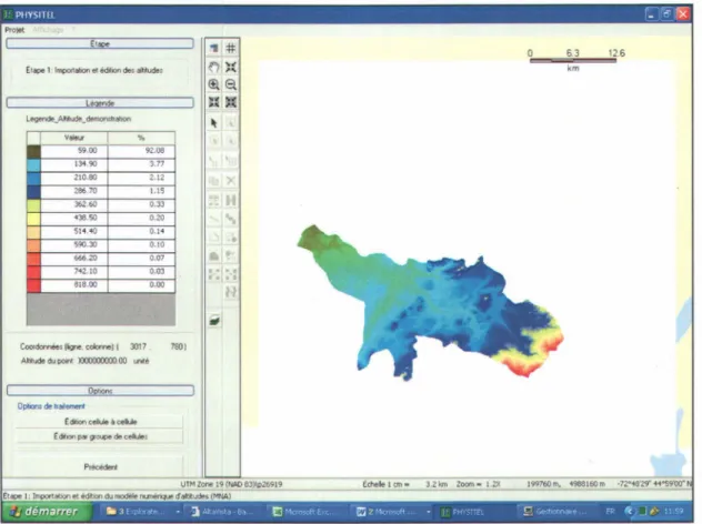
The fust step is the importation of the Yamaska watershed DEM which is based on a square grid with a resolution of 19m by 19m (see Figure 2.1).

ProJet Legende .... 92,06 '3.77 2.12 1.15 0.33 0.20 0.14 0,10 0,07 0.03 0.00

Coooclamêes (ligne c:oIomei (3017 780)

Altf<.ode du poo! :ro:KXXXXXl.OO ...

OotlOnS (dooon ... àc ... tdillOrl~lJ~dec~$ " :Il: ~ ~~ ~, <±tEl. CO

,

•

·

•

..

UlM Zone 19 (NAD 83)11'26919

Ét .... 1: ,,,,,,,,,.tian et édition du modèle.-...rh,.,. daitttudes (MNA)

6.3 12.6

km

Échele 1 cm - 3.2 km Zoom - 1.ZX

Figure 2.1 : Importation and edition of the initial DEM of the Yamaska river watershed.

2. PHYSlTEL Software and TI Computation 5

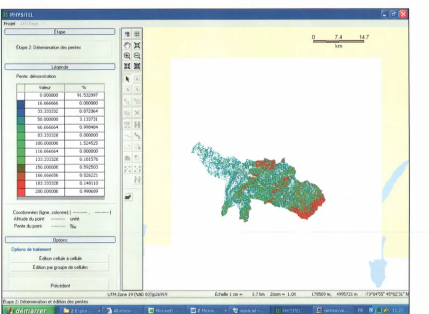
The second step generates a slope matrix (see Figure 2.2). For the D8 algorithm, the slope is calculated as foilows:

e -e

slope

=

den (2.1)

Where ee and en are respectively elevations of the central ceil and its neighbouring ceil. den is

the distance separating the centers of these two ceils.

Step 3 focuses the importation and ail functionalities for the edition of the initial DRLN (see Figure 2.3). This stage is prior to the rasterization of the DRLN vector map. The DRLN must be pre-treated to create a fully dendritic drainage network. Therefore, the connectivity between ail the stream network segments must be ensured.

In order to achieve this task, the foilowing steps must be taken:

(i) Ail off-stream network lakes and linear features that are not connected to the stream

network have to be removed. It is evident that these lakes and stray stream segments should be

without great influence on the drainage structure of the watershed;

(ü) In-stream lakes must be converted to closed polygons;

(fi) Ail streams in the DRLN that have a left and a right bank must be replaced by a single arc in the center of stream. If the river is thinner than the grid resolution it is sufficient to keep one of the two ridge lines of the river;

(iv) The main stem of the drainage network must extend to the edge of the corresponding DEM. Then, the location of the watershed outlet has to be determined and

PIIYSllIl ~-:J~ I~ Projet

(tape 2: Déte", .. w"", des pentet

légende Perle d&oons~at"", 'X H

...

••

Coofllonnée:liogne, colome) ( _ ... , ... __ . ) Al~ude du poont. unoté

Perle du pool _._ .• - %0

Dpt""" de ~aiI~

E<hln celule à ceIuIe

(dot"", pal !lf"'4l" de ceL4es

Précedent

Étape 2: Oéterll'liMtlon et édition des pentes

UTM Zone 19 (NAD 83)\p26919 Échele 1 cm - 3.7 km Zoom - LOX

o 74

km

147

178S09 m. ~995nl m -73"0'1'55" ~5"02'31·

2. PHYSlTEL Software and TI Computation

PtlYSllll . _ -... l'X

Projet

L~ (dibonvedonei

h40de ~dltlOnde:J veda ..

~e\Regoons

ElOmeriédolel>le

NO<Udvui>le. NO<Ud,~dé<>Ioçel>le

Noeud> ~

eIIaçable.-Additoon de noeuds pouille.

Non Non Ne» Non

Coo«b""" (ione. cdonnoll 2127 1359 J

Alt.ude du .,..,. 281 00 unoIé

P ... du.,..,. 104 %0

0"'",",

0 ... de ...

Ae1tNOf La COIJeu des vedetAt

T e:t de connectrv(~ a partJ dun veda. Détecbon des rietsecbons SaN noeud sous-jaCent

CorrveftIIer~ferrn6asenlegou OétectlCn des

t.

Segmenter au>! IOf"ICbOnt Cetemw'lel' La pod.1On de rex\iœoe Test de comecc~é à parti de reKUlOle

OétectOl' let vecte\,n nort-COfYleKet Réonentahon des vectet..u Oétecbon des cydes et vec;1a.S S\()efDO&M

Vaidatl)t'l du RlbeauVeclc:rtellfl1)OSé

UTMZone

Etape 3: Importation ~ ècibon du réseau vectorlellf'l'lPQSe

tCheIelcm- 1.9km Zoom-2.OX

Figure 2.3 : Importation and edition of the DRLN of the Yamaska watershed.

7

Step 4 consists in converting the DRLN vector resulting from step 3 to a raster representation

8 Computa tional Procedure of the Topographie Index U sing PHYSITEL

PIIYSIIII '" '", lx

""")0<

1

COOI_(i"n"",,,I,,m.~1 2005. 1295) Al<ude du por;. JOOOOO.OO ...

Pente du por;. 1 %0

OptlOrlt

0"""", de ."ement

RettNC!f la couleul des vec:teu$

Detefrnrlel ta posAton de rexutore

DetectIOn dea cycles el vecle\JI$ $oper~t

Valdatton du Rmau Malllctelltnp01ê

Chao"."" .. ... 001

5 _ " " 1 S"","",,,,"" 2

5 - , , " , 3

UlM Zone 19 (NAD fl3)\pZ6919

Etape 1: Oéterrmaoon et édit;" du réseau mMnclei imposé <

38

km

l CM- 1.9km Zoom- 2,QX

Figure 2.4 : Rasterization and edition of the DRLN of the Yamaska watershed.

75

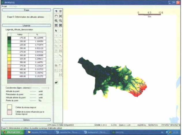
The DEM "burning" pro cess cornes in step 5. This process effectively digs a trench in the DEM following the DRLN (see Figure 2.5). This task is done by subtracting a perturbation coefficient from the original elevations of the DEM. Note that, this process is restricted to a buffer zone around the DRLN raster which is determined by a maximum radial influence parameter.

2. PHYSlTEL Software and TI Computation

PIIVSIIII _ '" l'X

Prolet

El..,.

-" =II:

Elo!JC)e 5 Détefll'WlatlOf'l des-aMcude: aIIétèes

o

!±ta Légende ~G Leoendo_Al<ude_demono.""" _~ Vtle<z

...

I

~

..

•

.,

CelM ÔJ leteau ImpOse

C_ de la ... rIluerdo par le

léfe411llf1)O$e

OptIOnS

UTM20ne 19 (NA083)\026919 Ét..,. S, Dé<emw>otlon et ~ du ~...,.. .... dattudes ""é<è

-Figure 2.5 : DEM "burning".

63 126

km

Echele 1 cm - 3.2km Zoom - 1.2X

9

The flow direction matrix is generated in step 6 (see Figure 2.6). It is noteworthy that the

simulation cime of this step and for the Yamaska river watershed (3185 columns X 3021 rows)

took 17.5 hours using a Pentium 4 CPU which has 2.8 Ghz of frequency and 480 Mo of RAM.

10 Computational Procedure of the Topographie Index Using PHYSITEL PIIYSlTIl ': ';~ rx p,ojet 1

..

œ.a

n

•

•

El'-•

₀

•

•

•

ot...

----

...

...

p.,...ot...

--

Reonentahon dlA'l grOl..C)e 't'en: t.rIe œIJe

0 _ dot or .... .oon. ondét",nw>ées Oètecbon dM or1ef"llatJont Oœeet ou opposées

Correcbcn dei Oflental:lOO$ CICIIlee, ou ~ées

Détecbon det c)des '0

Oéten,wleIla pemhon de rext,iOle

lITMZono 19 (NA083)\P26919

ÉtCle": DéterrMabon et èdition ÔJ '!"Seau rMtrldet mposé

-Echele 1 cm - 3.21cm Zoom - I.ZX 128194 m, 5069185 m

Figure 2.6 : DeteIDÙnation and eclition of the flow direction mat:t:.L"'{.

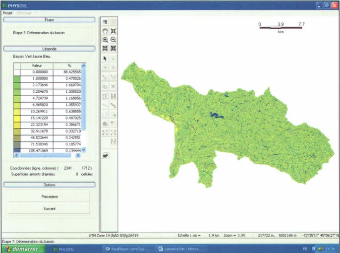
Finally, step 7 is declicated to the generation of the flow accumulation matrix on the basis of

the flow direction matrix (see Figure 2.7). The upstream of each grid cell is computed by accumulating cells that flow through this given cell. The cells draining an area greater than a

2. PHYSlTEL Software and TI Computation 11

ProJOt

~I..,. _'1

0 39 7.7

El..,. 7' Détoflr,no!",,';" bof.in f'I "

....

(±te Léoendo

==

COOfdomée< (ligne. colome) ( 2341. 1712)

S-,I",oo. amont. chInée.. 0 _

Pcécédenl

S ... ant

UlM Zone 19 (NAD 83)\p26919 Echele 1 cm - 1.9 km Zoom - 1.9X 217722 m..c 5001186 m ·72"35'17' 45'06'27" N

Figure 2.7: Determination of the flow accumulation matrix.

2.2 CALCULATION OF

TI ON

THE YAMASKA

WATERSHED

2.2.1 Methodology

The computation of TI distribution lS performed by Arc GIS 8.3. Preliminary steps are

necessary: The slope and flow accumulation matrices generated by PHYSITEL need to be imported into Arc GIS. This task is done on the basis of the following steps:

(i) Slope and flow accumulation are generated by PHYSITEL in text files format; (ii) Creation of headers to these two files;

(iii) Replacement of points by commas;

(iv) Modification of the extension of the Slope and flow accumulation files from .txt to .asc and

12 Computational Procedure of the Topographie Index U sing PHYSITEL

(v) Conversion of these two flles by Arc Tooi Box to grid fùes format which is compatible with Arc GIS.

Finally, TI is calculated by the "Raster Calculator" window as follows:

TI

=

In[(jzOW ace]

+

1]

[slp]

+

1000

(2.2)

Where,

(jzow _ ace]

[slp]

generated by the PHYSITEL.

2.2.2 Results and discussions

In this study, the TI distribution for the Yamaska watershed was calculated making use of a

slope and flow accumulation matrix that are generated by PHYSITEL. This result was

compared to the TI distributions calculated in a previous stlidy (Rousseau et aL, 2005) by the

D8-LTD (Orlandini et aL, 2003), D8-LAD (Tarboton, 1997) and D8 (O'callaghan and Mark,

1984) integrated in Arc Hydro Toois (see Figures 2.8 to 2.11). The influence ofDRLN is clear

on the map of TI distribution which is computed by PHYSITEL. In fact, the lakes are

successfully simulated within the Yamaska DEM which is burnt following the DRLN.

Regarding wide rivers with two banks, PHYSITEL offers a manual edition of the DRLN so that wide rivers are replaced by a central arc. In the vicinity of the watershed boundary, flat surfaces are sometimes undetermined during the flow direction generation step. However, within the PHYSIEL framework the user can manually assign arrows to cells of flat zones.

Figure 2.12 presents histograms of TI distributions for the Yamaska watershed which are

obtained by the different algorithms. The histograms which correspond to PHYSITEL and

D8-LAD do not contain negative TI values which correspond to high areas not contributing to

flow accumulation or when a<tanfJ (where a is the upslope area per unit contour length and

tanfJ is the slope). If we compare TI distributions as calculated by Arc Hydro Toois and

PHYSITEL which only differ by the way the DEM is burnt, the histograms are almost similar

with the exception that Arc Hydro generates negative values of TI. But if we cumulate the TI

values of [-2;0[ and [0;2[ classes generated by Arc Hydro we frnd 70% which is the same

value of TI distribution in the [0;2[ class using PHYSITEL. This could be explained by the fact

2. PHYSI1EL Software and TI Computation 13

Yamaska Watershed (Orlandini D8-L TD)

Resolution (

19

m )

Figure 2.8: TI distributions obtained by D8-LTD for the Yamaska nverwatershed (resolution 19m).

14 Computational Procedure of the Topographie Index Using PHYSITEL

Yamaska Watershed (Tarboton DB-LAD)

Resolution (

19

m )

Figure 2.9 : Comparison of TI distributions obtained by D8-LAD for the Yamaska river

2. PHYSlTEL Software and TI Computation 15

Yamaska Watershed (Arc Hydra 08)

Resolution (

19 m )

Figure 2.10 : Comparison of Tl distributions obtained by Arc Hydro (D8) for the Yamaska

16 Computational Procedure of the Topographie Index Using PHYSITEL

Yamaska Watershed (Physitel 08)

Resolution (

19

m )

Figure 2.11 : Companson of TI distributions obtained by PHYSITEL (D8) for the Yamaska

o

-2. PHYSlTEL Software and TI Computation

Ln (a/tanb) distribution on Yamaska watershed

• Orlandini: OB-L TD • Tarboton: OB-LAD o Arc Hydra: OB o Fhysitel: OB [ -2 ; O[ [0; 2[ [2; 4[ [4; 6[ [6; 8[ [ 8; 10[ [1 0 ; 12[ [12 ; 14[ [14 ; 16[ [16 ; 18] Ln (a/tanb) 17

Figure 2.12 : Histograms of TI distributions obtained by the D8-LTD, D8-LAD, D8 of Arc

I l I l

3 CONCLUSION

A new procedure for calculating the TI distribution by PHYSITEL was proposed in this study. Results for TI distribution for the Yamaska watershed are satisfactory. The approach of DRLN

integrated in PHYSITEL (Turcotte et aL, 2005) bypasses the problem associated with the

D8-LAD, D8-LTD and Arc Hydro methods which cannot route water through lakes and wide rtvers.

Flat surfaces near the watershed boundary still generate problems of flow direction but they can be manually corrected in PHYSITEL. Eventually, it is noteworthy that PHYSITEL requires a long simulation cime to generate the flow direction matrix.

4 REFERENCES

Rousseau, A.N., A. Hentati, S. Trembley, 2005. Computation of the Topographie Index on 16 watesheds in Quebec. Rapport nO R-800-f. INRS-ETE, La Couronne (Qc), Canada.

Saunders, W., 1999. Preparation of DEMs for use in environmental modeling analysis. ESRI User Conference,]uly 24-30, 1999, San Diego, California.

http://gis.esri.com/library/userconf/proc99/proceed/papers/pap802/p802.htm

Tarboton D.G., 1997. A new method for determination of flow directions and upslope areas in

grid digital elevation models. Water Resources Research, 33(2): 309-319.

Turcotte R., J.-P. Fortin, A.N. Rousseau, S. Massicotte, J.-P. Villeneuve, 2001. Determination of the drainage structure of a watershed using a digital elevation model and a digital river and lake

network. Journal rifHydrology, 240: 225-242.

O'Callaghan J.F. and D.M. Mark, 1984. The extraction of drainage networks from digital

elevation data. Comput. Vis. Graph. Image Process, 27: 323-344.

Orlandini S., G. Moretti and M. Franchini, 2003. Path-based methods for the determination of

non dispersive drainage directions in grid-based digital elevation models. Water Resources Research,