The role of planarity in connectivity problems parameterized by treewidth

For every p-pass Shellsort algorithm and every increment sequence, every subset of n!/2 n input permutations of n keys contains an input permutation that uses ⍀ ( pn 1⫹(1⫺⑀)/p

Their linearity properties were recently studied by Drakakis, Requena, and McGuire, who conjectured that the absolute values of the Fourier coefficients of an Exponential Welch

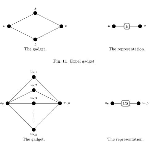
All sets of r distinct nodes host the same amount of exclusive data, independently of the choice of the r nodes. The fault tolerance mechanism can accommodate r −1 simultaneous

Ilias, Immersions minimales, premiere valeur propre du Lapla- cien et volume conforme, Mathematische Annalen, 275(1986), 257-267; Une ine- galit´e du type ”Reilly” pour

In this paper, we give a sharp lower bound for the first (nonzero) Neumann eigenvalue of Finsler-Laplacian in Finsler manifolds in terms of diameter, dimension, weighted

The existence of a positive lower bound of the compressi- bility is proved in the case of general quantum lattice systems at high temperature.. The compressibility

Its main result is an asymptotically deterministic lower bound for the PE of the sum of a low compressibility approximation to the Stokes operator and a small scaled random

This result by Reilly is a generalization, to Riemannian mani- folds of class (R, 0) (R > 0), of the well known theorem by Lichnerowicz [18 ] and Obata [21], which says that

References

1. H. L. Bodlaender, M. Cygan, S. Kratsch, and J. Nederlof. Solving weighted and counting variants of connectivity problems parameterized by treewidth deterministically in single exponential time. CoRR, abs/1211.1505, 2012.
2. P. Bonsma. Surface split decompositions and subgraph isomorphism in graphs on surfaces. In Proc. of the 29th International Symposium on Theoretical Aspects of Computer Science (STACS), volume 14 of LIPIcs, pages 531–542, 2012.
3. B. Courcelle. The monadic second-order logic of graphs. I. Recognizable sets of finite graphs. Information and Computation, 85(1):12–75, 1990.
4. M. Cygan, J. Nederlof, M. Pilipczuk, M. Pilipczuk, J. M. M. van Rooij, and J. O. Woj-taszczyk. Solving Connectivity Problems Parameterized by Treewidth in Single Exponential Time. In Proc. of the 52nd Annual IEEE Symposium on Foundations of Computer Science (FOCS), pages 150–159. IEEE Computer Society, 2011.
5. R. Diestel. Graph Theory. Springer-Verlag, 3rd edition, 2005.
6. F. Dorn. Planar subgraph isomorphism revisited. In Proc. of the 27th International Sym-posium on Theoretical Aspects of Computer Science (STACS), volume 5 of LIPIcs, pages 263–274, 2010.
7. F. Dorn, F. V. Fomin, and D. M. Thilikos. Fast Subexponential Algorithm for Non-local Problems on Graphs of Bounded Genus. In Proc. of the 10th Scandinavian Workshop on Algorithm Theory (SWAT), volume 4059 of LNCS, pages 172–183, 2006.
8. F. Dorn, F. V. Fomin, and D. M. Thilikos. Catalan Structures and Dynamic Programming in H-minor-free Graphs. In Proc. of the 19th annual ACM-SIAM Symposium on Discrete algorithms (SODA), pages 631–640, 2008.
9. F. Dorn, F. V. Fomin, and D. M. Thilikos. Catalan Structures and Dynamic Programming in H-minor-free graphs. Journal of Computer and System Sciences, 78(5):1606–1622, 2012.
Figure
Fig. 1. An illustration of a use of sphere cut decomposition.
Fig. 2. Color gadget.
Fig. 4. An example of H x graph with n x = 4.
Fig. 5. Maximal degree diminution to 5.
+7
Références
Documents relatifs