Alternative experimental method for characterizing the deformation behavior of Ti6Al4V at constant strain rates over the full elastoplastic range

International Journal of Material Forming

Alternative experimental method for characterizing the deformation behavior of Ti6Al4V

at constant strain rates over the full elastoplastic range

--Manuscript Draft--Manuscript Number: IJFO-D-19-00239

Full Title: Alternative experimental method for characterizing the deformation behavior of Ti6Al4V at constant strain rates over the full elastoplastic range

Article Type: IJMF 10th Anniversary - Advances in Material Forming Corresponding Author: Víctor Tuninetti

Universidad de La Frontera CHILE

Corresponding Author Secondary Information:

Corresponding Author's Institution: Universidad de La Frontera Corresponding Author's Secondary

Institution:

First Author: Víctor Tuninetti

First Author Secondary Information:

Order of Authors: Víctor Tuninetti Paulo Flores Marian Valenzuela Gonzalo Pincheira Carlos Medina Laurent Duchêne Anne-Marie Habraken Order of Authors Secondary Information:

Funding Information: Comisión Nacional de Investigación Científica y Tecnológica

(11170002)

Prof. Dr. Víctor Tuninetti Universidad de La Frontera

(DI17-0070) Prof. Dr. Víctor Tuninetti Universidad de La Frontera

(FRO1855) Prof. Dr. Víctor Tuninetti

Wallonie-Bruxelles International

(SUB2019/419031) Dr. Anne-Marie Habraken Fonds De La Recherche Scientifique

-FNRS Dr. Anne-Marie Habraken

Abstract: Full range constant strain rate tests are required for accurately characterizing initial yield point, strength differential effect and direct identification of constitutive laws describing the plastic behavior of materials. These tests require the use of a closed-loop control in order to achieve the constant strain rate, however this feature is not available in many laboratories. An alternative method is proposed here for full range constant strain rate with testing machines that can be configured for user-defined displacements of the cross head prior to testing. Tests performed at a constant die speed include a variable strain rate response for the specimen involved. Significant deformation rate variation occurs between the elastic and plastic range with consequences for initial yield point identification. To overcome this drawback, appropriate user-defined displacements can be computed and applied, allowing for

well as a 3D digital image correlation (DIC) system exhibiting a constant strain rate value equal to 10-3 s-1, for both elastic and plastic ranges. A non-negligible inhomogeneous strain field was measured on the surface of the compression specimen using DIC and was corroborated by numerical modeling. Results identified the source of the non-homogeneous strain field, thereby proposing a quantitative indicator of plastic anisotropy. The initial yield stress and strain hardening rates of the alloy at several temperatures were obtained with both testing method, conventional constant cross-head speed, and the constant strain rate; these were then used to determine the influence of the small strain rate variations on the mechanical response of Ti6Al4V alloy.

Alternative experimental method for characterizing the deformation behavior of Ti6Al4V at constant strain rates over the full elastoplastic range

Víctor Tuninettia*, Paulo Floresb, Marian Valenzuelac, Gonzalo Pincheirad, Carlos Medinab, Laurent Duchênee, Anne-Marie Habrakene,f

a _{Department of Mechanical Engineering, Universidad de La Frontera, Francisco Salazar}

01145, Temuco 4780000, Chile

b _{Department of Mechanical Engineering, Universidad de Concepción, Casilla 160 – C,}

Correo 3, Ciudad Universitaria, Concepción 4030000, Chile

c _{Department of Civil Engineering and Geology, Universidad Católica de Temuco,}

Rudecindo Ortega 02950, Temuco 4780000, Chile

d _{Department of Industrial Technologies, Universidad de Talca, Los Niches km 1,}

Curicó 3340000, Chile

e _{ArGEnCo Department, MSM team, University of Liège, Quartier POLYTECH 1, allée}

de la Découverte 9, Liège 4000, Belgium

f _{Fonds de la Recherche Scientifique – F.N.R.S.–F.R.S., Belgium}

*Corresponding author: victor.tuninetti@ufrontera.cl; tel.: + 56452325984.

Acknowledgements

The authors thank the Chilean Scientific Research Fund CONICYT FONDECYT 11170002, the Universidad de La Frontera Internal Research Fund DIUFRO (Project DI17-0070), the Marco multiannual convention FRO1855 and the cooperation agreement WBI/AGCID SUB2019/419031 (DIE19-0005). As research director of FRS-FNRS, A.M. Habraken thanks the Belgian Scientific Research Fund FNRS for financial support. The authors would also like to thank O. Milis for his technical support.

Manuscript Click here to access/download;Manuscript;Manuscript.docx

1 2 3 4 5 6 7 8 9 10 11 12 13 14 15 16 17 18 19 20 21 22 23 24 25 26 27 28 29 30 31 32 33 34 35 36 37 38 39 40 41 42 43 44 45 46 47 48 49 50 51 52 53 54 55 56 57 58 59 60 61

Abstract

Full range constant strain rate tests are required for accurately characterizing initial yield point, strength differential effect and direct identification of constitutive laws describing the plastic behavior of materials. These tests require the use of a closed-loop control in order to achieve the constant strain rate, however this feature is not available in many laboratories. An alternative method is proposed here for full range constant strain rate with testing machines that can be configured for user-defined displacements of the cross head prior to testing. Tests performed at a constant die speed include a variable strain rate response for the specimen involved. Significant deformation rate variation occurs between the elastic and plastic range with consequences for initial yield point identification. To overcome this drawback, appropriate user-defined displacements can be computed and applied, allowing for both tensile and compression tests to be performed at a constant strain rate. The method is validated using a compression test of Ti6Al4V alloy at room temperature, as well as a 3D digital image correlation (DIC) system exhibiting a constant strain rate value equal to 10-3 s-1, for both elastic and plastic ranges. A non-negligible inhomogeneous strain field was measured on the surface of the compression specimen using DIC and was corroborated by numerical modeling. Results identified the source of the non-homogeneous strain field, thereby proposing a quantitative indicator of plastic anisotropy. The initial yield stress and strain hardening rates of the alloy at several temperatures were obtained with both testing method, conventional constant cross-head speed, and the constant strain rate; these were then used to determine the influence of the small strain rate variations on the mechanical response of Ti6Al4V alloy.

Keywords: Strain rate sensitivity; Constant strain rate test; Stress–strain curve; Digital

image correlation; Ti6Al4V.

1 2 3 4 5 6 7 8 9 10 11 12 13 14 15 16 17 18 19 20 21 22 23 24 25 26 27 28 29 30 31 32 33 34 35 36 37 38 39 40 41 42 43 44 45 46 47 48 49 50 51 52 53 54 55 56 57 58 59 60 61

1. Introduction

The macroscopic mechanical characterization of large deformation behavior of Ti6Al4V alloy involves the identification of an initial yield locus, as well as defining how its evolution is affected by plastic work, strain path, temperature, and strain rates [1–4]. Several isotropic hardening laws representing the evolution of the yield locus are available in the literature, including the isotropic Zerilli–Armstrong [5], Norton–Hoff [6], and the most widely used Johnson–Cook [7–9] (JC) laws. The characterization of these constitutive laws requires mechanical tests such as uniaxial tensile [10–14] or compression tests [15–19]. To accurately identify these constitutive laws using a direct method, both compression and tensile tests must be performed, not only at constant temperatures as demonstrated by Galán-López et al. [20], but also at constant strain rate values [21]. Universal testing machines equipped with Proportional Integral Derivative (PID) controllers are commonly used to perform constant strain rate tests by monitoring and controlling the actuator or the crosshead displacement [22]. However, the machines available in many laboratories do not offer this capability; and they are limited to the configuration for ramping, sinusoidal, or user-defined displacements of the cross head prior to testing. Hereafter, the latter capability is used to develop a procedure for constant strain rate tests by computing the appropriate user-defined displacements. A compression test of Ti6Al4V alloy has been selected to present this method, which can be applied for compression or tensile testing.

The average true axial compression strain in a sample as a function of time is defined as in Eq. 1:

 

 

_        0 0 ln H t X H t ep



, (1) 1 2 3 4 5 6 7 8 9 10 11 12 13 14 15 16 17 18 19 20 21 22 23 24 25 26 27 28 29 30 31 32 33 34 35 36 37 38 39 40 41 42 43 44 45 46 47 48 49 50 51 52 53 54 55 56 57 58 59 60 61

where,

H

₀ is the initial height of the specimen, and X_ep

 

t is either the elongation (positive values) or shortening (negative values) of the specimen.

The strain rate  can be computed by applying the derivative

 



     dt d to Eq. 1:

 



dt

 



t X d t X H ep ep   0 1  . (2)

By reordering Eq. 2 and assuming a constant  , the differential equation Eq. 3, and its solution Eq. 4, can therefore be obtained:

 





_{ }

0

0









X

t

H

dt

t

X

d

ep ep



_



_

, (3)

 

t H0



exp

 

t 1



Xep



 . (4)

From Eq. 4, time t can be computed as a function of the known value of the shortening

of the specimen Xep

 

t (elongation for tensile):

 

        0 0 ln 1 H t X H t ep  . (5)

Eq. 4 allows for the displacement to be computed as a function of time, Xep

 

t , which

is necessary to impose on the sample for a required test at a constant strain rate, . It should be noted that Xep

 

t can only be employed as the user-defined displacement if the

cross head is controlled according to the displacement, as measured by an extensometer that is directly applied to the specimen. This is generally the case for tests performed with a tensile testing machine at room temperature (RT). Subsequently, a constant strain rate can be obtained by imposing user-defined displacement, as computed with Eq. 4, in the

1 2 3 4 5 6 7 8 9 10 11 12 13 14 15 16 17 18 19 20 21 22 23 24 25 26 27 28 29 30 31 32 33 34 35 36 37 38 39 40 41 42 43 44 45 46 47 48 49 50 51 52 53 54 55 56 57 58 59 60 61

gauge zone of the extensometer. However, it should be noted that high-temperature extensometers for tensile tests are not always available. Additionally, concerning those testing machines generally used for compression tests, the sensor associated with the user-defined displacement is often connected to the cross head. In these two cases (compression tests and high-temperature tensile tests), the rigidity of the machine should first be identified and considered, as this allows for the appropriate displacement or deformation of the specimen to be imposed for the constant strain rate tests.

The load associated with the cross-section of the tested sample may reach a high value, particularly on those alloys with a high yield strength (such as Ti6Al4V) [23, 24]. Consequently, this high load produces a non-negligible deflection of the testing machine’s components, and this must be considered when computing the user-defined displacement of the cross head. It is important to note that the rigidity of the machine relies on the configuration of the dies, the position of the cross head, and the testing temperature. Accordingly, rigidity should be measured after change to the initial configuration of the machine or testing environment has taken place.

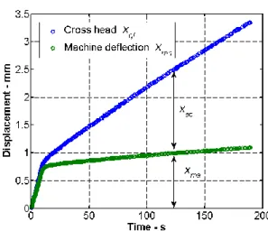
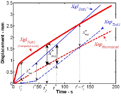
Imposing a cross head global displacement Xgl

 

t with the aim of reaching a specific specimen shortening (elongation for tensile) Xep

 

t requires previous knowledge of

machine deflection

X

ma

 

t

(Fig. 1). This deflection could be measured during the testing

of a sample of a specific material; however,

X

_ma

 

t

depends on the load applied by the machine, which itself depends on the material’s strain rate sensitivity.

In conducting a single constant-strain rate test without knowledge of the behavior of the material, the first option is to use the closed-loop control feature (PID controller) [21]. A PID controller calculates an error as the difference between a measured strain rate and

1 2 3 4 5 6 7 8 9 10 11 12 13 14 15 16 17 18 19 20 21 22 23 24 25 26 27 28 29 30 31 32 33 34 35 36 37 38 39 40 41 42 43 44 45 46 47 48 49 50 51 52 53 54 55 56 57 58 59 60 61

the desired value. The controller then attempts to minimize the error by adjusting the speed of the cross head.

Fig 1. Deflection of the servo-hydraulic 400 kN universal testing machine (Schenck Hydropuls) and deformation of a Ti6Al4V specimen in a constant cross head speed test at v0.021 mm/s.

A second option, which is explained in the following section, is to perform a series of consecutive tests. The number of tests needed to attain a constant strain rate test will vary according to the sensitivity of the specimen-machine system which is composed by both the machine rigidity and strain rate sensitivity of the tested material. Concerning Ti6Al4V and the rigidity of the machine used herein, a constant strain rate was reached during the second test.

2. Experimental procedure

2.1. Test at a constant strain rate

Briefly, the method for constant strain rate tests comprises three steps: (a) identification of the stiffness of the machine; (b) identification of the behavior of the system machine-specimen by performing a test of the material sample at a constant cross head speed; and (c) computation of the appropriate global displacement for application to

1 2 3 4 5 6 7 8 9 10 11 12 13 14 15 16 17 18 19 20 21 22 23 24 25 26 27 28 29 30 31 32 33 34 35 36 37 38 39 40 41 42 43 44 45 46 47 48 49 50 51 52 53 54 55 56 57 58 59 60 61

the cross head during testing to achieve constant strain rate over the full range of strain, both elastic and plastic, by using the two sets of data obtained in steps (a) and (b). A detailed description of these steps will now be given, along with valuable information pertaining to the application of this method.

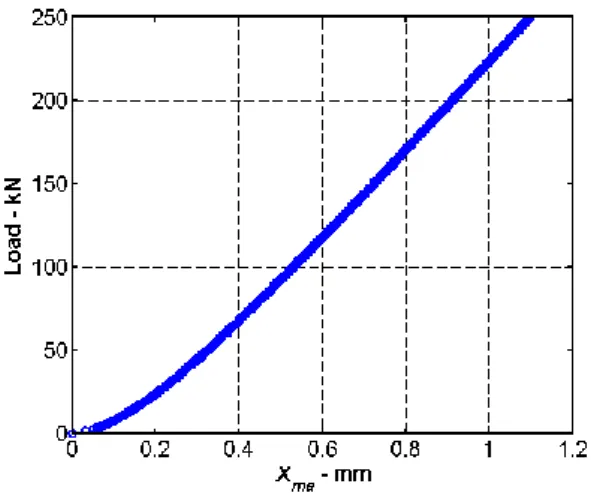
(a) Identification of the stiffness of the testing machine. A die compression test, without

the use of a specimen, is performed to obtain the load-deflection curve of the testing machine at a specific cross head position and testing temperature. Fig. 2 shows the characteristic shape of the load-deflection curve of the testing machine at RT. It should be noted that, for the tensile test, the curve of the testing machine can be obtained by performing a test on a material sample using a gauge length close to zero. This configuration allows for the machine’s deflection to be measured due to the negligible elongation of the sample.

Fig 2. Example of a load-deflection curve of the testing machine (SCHENCK Hydropuls 400 kN press) for a specific compression configuration at RT.

(b) Identification of the behavior of the system machine-specimen. The sample is tested

at a constant cross head speed (test 1) to obtain the deflection response of the system machine-sample. For this test, the constant die speed must be defined in such a way that the strain rate obtained using the sample is as close as possible to the targeted constant

1 2 3 4 5 6 7 8 9 10 11 12 13 14 15 16 17 18 19 20 21 22 23 24 25 26 27 28 29 30 31 32 33 34 35 36 37 38 39 40 41 42 43 44 45 46 47 48 49 50 51 52 53 54 55 56 57 58 59 60 61

strain rate. This die speed is computed as the ratio between the final global displacement of the cross head Xgland the test duration t (Eq. 6), thereby incorporating the expected

machine deflection,

X

ma, t X X t X v gl ep ma      . (6)

As the average targeted strain rate  during the test is defined as the variation in the strain 



( _F, assuming an initial strain



0



0

) for a certain time duration t

(Eq. 7), tcan be obtained using Eq. 8:

t      (7)       F t   (8)

By substituting Xep computed from Eq. 4, at the end of the test, and by substituting

t

 from Eq. 8 into Eq. 6, the expression for the average die speed in test 1 at a constant cross head speed becomes:

 





F ma F X H v







    0 exp 1 , (9)

where

X

_ma corresponds to the total final deflection of the machine. This value is obtained from Fig. 2 (machine rigidity) by knowing the expected load during the test; here, the expected load value is derived from the strength of the material. The value approximated by multiplying the mean value between the initial yield stress and the maximum expected engineering stress of the tested material (as taken from the literature value) with the cross-sectional area of the sample. To determine the shortening of the

1 2 3 4 5 6 7 8 9 10 11 12 13 14 15 16 17 18 19 20 21 22 23 24 25 26 27 28 29 30 31 32 33 34 35 36 37 38 39 40 41 42 43 44 45 46 47 48 49 50 51 52 53 54 55 56 57 58 59 60 61

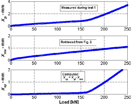
specimen (elongation in tensile) Xep, the load-deflection curve of the testing machine

ma

X

and the load-displacement curve (Xgl in Fig. 1) in test 1 must be set at identical load-sampling frequencies (Fig. 3).

Once Xep is known, the strain is obtained using Eq. 1 and the stress is automatically computed by assuming volume conservation and no barreling (Eq. 10):

 





   exp 0 A F , (10)

where, Fis the measured load and

A

₀ is the initial cross-sectional area of the sample.

This procedure, implemented in an independent script, can be used to automatically obtain the stress–strain curves from data generated by the universal testing machine.

Fig. 3. Displacement vs. load curves at identical load sampling frequencies: (a) constant cross head speed test (test 1), (b) deflection vs. load curve of the machine, and (c)

1 2 3 4 5 6 7 8 9 10 11 12 13 14 15 16 17 18 19 20 21 22 23 24 25 26 27 28 29 30 31 32 33 34 35 36 37 38 39 40 41 42 43 44 45 46 47 48 49 50 51 52 53 54 55 56 57 58 59 60 61

computed shortening of the specimen Xep XglXma, for the case v0.021 mm/s, targeted 1103 s–1.

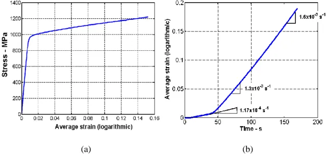
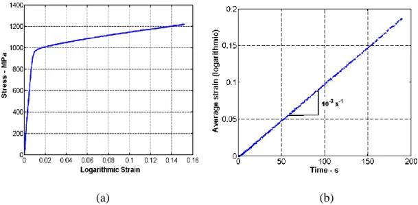
Fig. 4 shows the stress–strain and strain–time curves obtained in test 1. Fig. 4b shows that the strain rate reached during test 1 is far from constant. The elastic strain rate differs significantly from the targeted value (1.17×10–4 s–1 instead of 1.0×10–3 s–1) because, in this domain, the load increases at a higher rate than in the plastic domain, producing significant increase of the machine deflection. However, when the sample becomes plastic, the load increases at a lower rate owing to the strong decrease of the strain hardening rate of Ti6Al4V. This lower increase of the load induces a reduction of the machine deflection and, therefore, a strain rate closer to the targeted value. However, this strain rate is still not constant, particularly at the onset of plasticity, which is a key feature in many material models.

(a) (b)

Fig. 4. (a) True axial stress–strain curve, (b) true axial strain–time curve at constant cross head speed whenv0.021 mm/s, and targeted 1103 s–1.

1 2 3 4 5 6 7 8 9 10 11 12 13 14 15 16 17 18 19 20 21 22 23 24 25 26 27 28 29 30 31 32 33 34 35 36 37 38 39 40 41 42 43 44 45 46 47 48 49 50 51 52 53 54 55 56 57 58 59 60 61

(c) Computation of the appropriate global displacement for the test at a constant strain rate. Here, the objective is to determine the user-defined displacement

 

Xgl , as a function of time, in such a manner that the shortening of the specimen



Xep_ TEST2



computed by Eq. 4 follows the required or theoretical value necessary to achieve the test at a constant strain rate  , over the full range of strain (Fig. 5).

First, the behavior of the system machine-specimen



Xma



Xep,









at a constant strain

rate, equal to 10–3 s–1 for the chosen case, must be known to determine the appropriate user-defined displacement of the cross head Xgl_TEST2

 

t for the constant strain rate test. The exact behavior cannot yet be accurately known because the compression test has yet to be performed at the targeted constant strain rate. However, the behavior of the system-machine at a constant cross head speed is assumed to be similar to that observed in the targeted constant strain rate test (Eq. 11).



gl_TEST2



ma



gl_TEST1



ma X X X X  (11) 2 _ TEST gl

X should be determined as a function of time, which is referred to as t2. Time t2 is computed by shifting curve Xgl_ TEST1 (for any point at time t*) over the time difference between the curves Xep_ TEST1 and Xep_TEST2THEORETICAL (t*2–t*) (see arrows from t* to t*2 displayed in Fig. 5). This computation is carried out with the assumption

that there is no variation of the system-machine behavior (Eq. 11). Consequently, for a certain shortening value, the time at which global displacement is applied changes from

t* to t*2; that is, Xep_TEST2

 

t2  Xep_TEST1

 

t1 . A similar estimated shift is then applied to all other points, as observed for the two examples tand o

t , by using Eq. 12 (adapted from Eq. 5). 1 2 3 4 5 6 7 8 9 10 11 12 13 14 15 16 17 18 19 20 21 22 23 24 25 26 27 28 29 30 31 32 33 34 35 36 37 38 39 40 41 42 43 44 45 46 47 48 49 50 51 52 53 54 55 56 57 58 59 60 61

 

        0 1 _ 0 2 ln 1 H t X H t ep TEST  (12)

Fig. 6b shows that the theoretical shortening of the sample is obtained and the desired constant strain rate for the full strain range is reached by imposing the user-defined displacementXgl_TEST2

 

t2 in test 2.

Fig. 5. Schematic representation of the user-defined displacement computation achieved by shifting the Xgl_ TEST1 curve over the time difference betweenXep_ TEST1 and

THEORETICAL

ep

X .

It should be noted that in using this method, barreling of the sample is neglected and the strain computed is an average value of the local strains in the sample. It is necessary to verify the accuracy of the computed strain value with a local strain measuring technique. Section 2.2 presents a detailed procedure based on a three-dimensional digital

1 2 3 4 5 6 7 8 9 10 11 12 13 14 15 16 17 18 19 20 21 22 23 24 25 26 27 28 29 30 31 32 33 34 35 36 37 38 39 40 41 42 43 44 45 46 47 48 49 50 51 52 53 54 55 56 57 58 59 60 61

image correlation; this procedure is applied to obtain an accurate local strain field on the free surface of the compression sample, showing a non-homogeneous strain distribution.

(a) (b)

Fig. 6. (a) Compressive axial true stress – axial true strain curve (absolute values), (b) axial true strain time curve at constant strain rate 1103 s–1 for a sample of Ti6Al4V tested while imposing the user-defined displacement Xgl_TEST2

 

t2 .

2.2. Strain field measurement by digital image correlation

The development of digital image correlation (DIC) and its combination with stereovision principles, allows measurement of the displacement and strain field evolution of tested specimens. Similar to human vision, two imaging sensors focus on an object from different positions and thereby provide enough information to perceive the object as three-dimensional. Using a stereoscopic camera setup, each object point is represented on a specific pixel on the image plane of the respective camera. With the knowledge of each camera’s imaging parameters (intrinsic parameters: focal length, principle point, and distortion parameters) and the orientations of the two cameras with respect to one other (extrinsic parameters: rotation matrix and translation vector), the position of each object point can be calculated in 3D [25]. These data are very useful, not

1 2 3 4 5 6 7 8 9 10 11 12 13 14 15 16 17 18 19 20 21 22 23 24 25 26 27 28 29 30 31 32 33 34 35 36 37 38 39 40 41 42 43 44 45 46 47 48 49 50 51 52 53 54 55 56 57 58 59 60 61

only for model-validation purposes, but also for identifying material parameters through the inverse-identification method. A complete review of the essential concepts underlying the use of the 3D-DIC can be found in Palanca et al., [26].

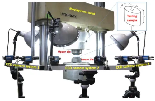
Commercial Vic3D DIC software (Correlated Solutions Inc., Columbia, SC, USA) and the Limess (Limess Messtechnik und Software GmbH, Pforzheim, Germany) system were used to measure the displacement/strain fields in the compression tests (Fig. 7). To validate the proposed method for constant strain rate tests seen in Section 2.1, an experimental methodology was developed and successfully applied to accurately determine the cross-sections, the displacement/strain field evolution of the samples, the true stress–true strain, and, in particular, the strain–time curves.

Fig. 7. Universal testing machine equipped with a contactless 3D-DIC strain measurement system (six CCD cameras) based on digital image correlation for compression tests.

Accurate DIC results are difficult to obtain because extensive knowledge, experience, and high levels of technical and practical skills are required. Errors often affect measurements obtained by DIC systems, and an optimization of the numerical process

1 2 3 4 5 6 7 8 9 10 11 12 13 14 15 16 17 18 19 20 21 22 23 24 25 26 27 28 29 30 31 32 33 34 35 36 37 38 39 40 41 42 43 44 45 46 47 48 49 50 51 52 53 54 55 56 57 58 59 60 61

and a validation of the experimental results are always required [26]. The main solutions for managing difficulties in obtaining accurate and reproducible compression test data with the 3D-DIC system are:

 Adequate ductility of paint. Various brands and types of spray paint were tested before the optimal paint was identified. An appropriate paint ductility is required so that large displacements and strains among the specimens can be followed until the onset of fracture. Many spray paints available on the market were unsuitable because, during testing, paint cracks appeared long before the specimens fractured. Ductility of the paint rapidly changes with time from the instant it is applied. The later the tests were performed, the lower the ductility of the paint. The MoTip Heat-Resistant (www.motip.com) spray paint was selected because it showed excellent adhesion and ductility.

 Appropriate subset size and optimal size of black dots for the speckle pattern. Optimal speckle coverage is 40–70 % [27]. Stickers were developed in the Mechanics of Materials and Constructions department (Vrije Universiteit Brussel) using an optimized printed speckle pattern. Subsequently, these were tested with the specimens studied but yielded no accurate results owing to a lack of ductility in the plastic and the adhesive. However, an optimal size when using spray paint was identified and applied accordingly; the smallest possible subset was selected, with sizes ranging from 3 x 3 to 10 x 10 pixels.

 Fixing cables and camera supports. Any relative movement of the cameras modifies the calibration parameters and generates inaccuracies regarding the reconstructed 3D shape. Vibrations and relative movement between two cameras in the same system were eliminated by fabricating dedicated supports (Fig. 7a).

1 2 3 4 5 6 7 8 9 10 11 12 13 14 15 16 17 18 19 20 21 22 23 24 25 26 27 28 29 30 31 32 33 34 35 36 37 38 39 40 41 42 43 44 45 46 47 48 49 50 51 52 53 54 55 56 57 58 59 60 61

 Adequate lighting. To avoid high numbers of errors in the correlation and computation of the strain fields, several lamps were tested at different positions. A cold light was obtained using a StudioMax™ Daylight Kit 600/600 (30-Watt bulbs) manufactured by FotoQuantum® (Spain) (Fig. 7a). No strong light reflections appeared on the image. The testing environment was also isolated to avoid changes in the brightness of the image, and to prevent the loss of the image correlation sequence.

 Highest experimental resolution. Experimental resolution is defined as the measured distance along one pixel, which varies according to the distance between the cameras and the specimen, as well as the focus of the lenses. CCD-Limess cameras with 50 mm lenses were used. Extension tubes of 10 mm were added between the lens and the camera body, which allowed the sample to be closer to the cameras, improving the resolution of the images to 30 µm/pixel and therefore the accuracy of the results.

 Aperture, exposure time, and focus. The aperture, or size of the lens opening, allows for the adjustment of the amount of light received by the camera sensor. The focal length of the lenses is used to provide a sharp focus on the specimen; a larger aperture makes the image brighter, but also decreases the depth of field (i.e., the range over which the focus is sharp). Exposure time is the period over which the camera sensor collects light before reading a new image. Longer exposure times make images brighter but can also create blurring if significant sample-deformation occurs during this period. Several focuses, exposure times, and apertures were tested to obtain sharp images and to achieve accurate correlations. The optimal values found for compression and tension tests using the CCD-Limess cameras, with extension tubes of 10 mm and 50 mm, were f/5.6 for the

1 2 3 4 5 6 7 8 9 10 11 12 13 14 15 16 17 18 19 20 21 22 23 24 25 26 27 28 29 30 31 32 33 34 35 36 37 38 39 40 41 42 43 44 45 46 47 48 49 50 51 52 53 54 55 56 57 58 59 60 61

aperture, 15 ms for exposure time, and a 5–10 mm depth-of-field focus, which varied depending on the targeted point of the specimen.

3. Constant strain rate tests

3.1. Validation of the constant strain rate test method by digital image correlation

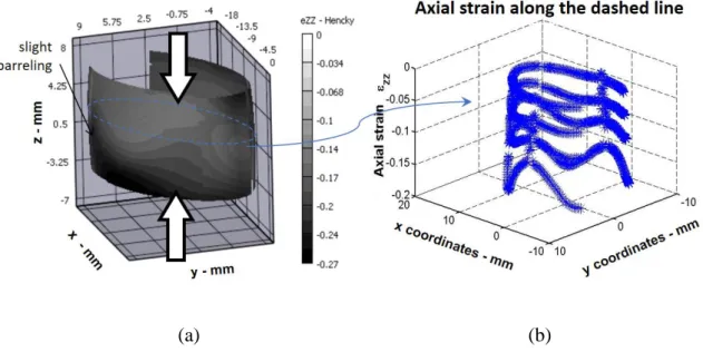
Fig. 7 shows the DIC system that was utilized to visualize and measure the strain field around the sample (Fig. 8a). Fig. 8b shows the distribution from which the mean axial compressive strain was computed. Fig. 9a shows the mean values of the axial strain compared with those obtained with Eq. 1 (computed with the shortening of the sample). Good agreement was found between the two strain computation methods; however, more a sample is deformed under compression, the higher the difference between the strain values will be, as computed using DIC and Eq. 1. This difference is related to the significant inhomogeneous strain distribution (Fig. 8b).

With digital image correlation, barreling can be considered when measuring stress evolution, which can be computed during the test, and when measuring the cross-sectional area. Specimen shortening measurements also allow for the cross-sectional area to be determined through consideration of volume conservation during plastic deformation, and a cylindrical shape neglecting barreling. Consequently, differences in the axial stress computation, varied according to their different data sources (Fig. 9b).

3.2. Analysis of the non-homogeneous strain field

The non-negligible inhomogeneous strain field on the surface of the specimen, as measured by DIC (Fig. 8b), could be related to the barreling of the specimen and the plastic anisotropy of the alloy. Numerical simulations of compression tests of elliptical cross-section specimens were performed with the aim of understanding this behavior.

1 2 3 4 5 6 7 8 9 10 11 12 13 14 15 16 17 18 19 20 21 22 23 24 25 26 27 28 29 30 31 32 33 34 35 36 37 38 39 40 41 42 43 44 45 46 47 48 49 50 51 52 53 54 55 56 57 58 59 60 61

Two types of constitutive laws, isotropic and anisotropic laws, were considered both with and without friction. The von Mises (VM) yield locus, identified by the compression test data in a previous work was used for the isotropic case [28]. The anisotropy of the material was modeled using the CPB06 yield criterion proposed by Cazacu et al., [29]. A description of the identification procedure, the set of material parameters of the CPB06 model, and the FE simulations can be found in Tuninetti et al, [30].

(a) (b)

Fig. 8. DIC measurements of the (a) final strain field of Ti6Al4V compression sample and the (b) evolution from the initial to the final load of the axial compressive strain distribution along the dashed line of the sample.

(a) (b) 1 2 3 4 5 6 7 8 9 10 11 12 13 14 15 16 17 18 19 20 21 22 23 24 25 26 27 28 29 30 31 32 33 34 35 36 37 38 39 40 41 42 43 44 45 46 47 48 49 50 51 52 53 54 55 56 57 58 59 60 61

Fig. 9. Comparison between (a) evolution of the mean axial compressive strain, computed from the distribution shown in Fig 8 and the average value taken from Eq.1; and, (b) compressive stress strain curves computed from volume conservation and measured cross-sectional area by DIC.

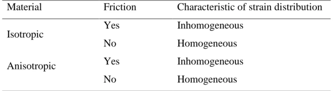
Fig. 10 shows the numerical and experimental axial strain distributions along the horizontal center line (dashed line, Fig. 8a) of the specimen. Simulation results show that, when friction is not considered, homogeneous strain fields are obtained for both isotropic and anisotropic materials. Additionally, when friction is considered, axial strain distributions obtained from the simulated test of the anisotropic case (CPB06) were found to be close to those of the experimental inhomogeneous strain. Therefore, it can be stated that friction enhances visualization of anisotropic behavior of a material in compression tests with an elliptic cylinder (Table 1).

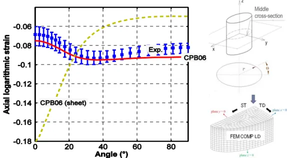
The sensitivity of the axial strain field to the plastic anisotropy was also verified by comparing the results of numerical simulations involving a dataset of: 1) a strong anisotropic sheet (r0=1.1 and r90=2.2) of Ti6Al4V alloy, and 2) the bulk alloy investigated

herein. The set of material parameters for the sheet was selected from those listed in Gilles et al. [31]. Fig. 11 shows that, compared to the bulk Ti6Al4V (CPB06), the axial strain distribution of the sheet compression (CPB06 sheet) obtained by the simulation presents a very high inhomogeneous strain field. Due to poor reliability, resulting from incomplete continuity between the sheet layers and significant scattering in the measurements, the experimental results from the sheet stack compression test are not shown; this test is better described in [32]. From these results, it can be concluded that the axial strain distribution in the compression test including friction is sensitive to the alloys’ plastic anisotropy (Table 2). However, this assumption should be further demonstrated with more experimental data. 1 2 3 4 5 6 7 8 9 10 11 12 13 14 15 16 17 18 19 20 21 22 23 24 25 26 27 28 29 30 31 32 33 34 35 36 37 38 39 40 41 42 43 44 45 46 47 48 49 50 51 52 53 54 55 56 57 58 59 60 61

Fig. 10. Assessment of the axial strain field predictions ezz (along the surface of the middle

cross-section) for a bulk Ti6Al4V alloy in a compression test for the LD direction.

Fig. 11. Assessment of the sensitivity of the axial strain ezz to the plastic anisotropy (along

the surface of the middle cross-section) for two Ti6Al4V alloys (bulk compression along LD direction and sheet compression in thickness direction).

Table 1. Effect of friction on the axial strain distribution of compression tests.

1 2 3 4 5 6 7 8 9 10 11 12 13 14 15 16 17 18 19 20 21 22 23 24 25 26 27 28 29 30 31 32 33 34 35 36 37 38 39 40 41 42 43 44 45 46 47 48 49 50 51 52 53 54 55 56 57 58 59 60 61

Material Friction Characteristic of strain distribution Isotropic Yes Inhomogeneous

No Homogeneous

Anisotropic Yes Inhomogeneous

No Homogeneous

Table 2. Axial strain distribution sensitivity to the anisotropy of the material in compression tests including friction.

Material Strain range Characteristic of strain distribution Isotropic [0.075; 0.1] Weakly inhomogeneous

Anisotropic [0.075; 0.095] Weakly inhomogeneous with a different shape than in isotropic case Strongly

anisotropic sheet [0.05; 0.18] Strongly inhomogeneous

4. Evaluation of the strain rate variation on the strain hardening of Ti6Al4V

The uniaxial compressive true stress–true strain curves of Ti6Al4V obtained at RT, 150 °C, 400 °C, 600 °C with both method, the constant crosshead speed and the constant strain rate are compared in Fig. 12. The first method based on the with Eq. 9 is set to reach a targeted average strain rate equal to 10–3 s–1. The second method presented in Section 2 was used to performed the constant strain rate test equal to 10–3 s–1.

The first method provides two merely constant strain rates for the plastic range (approximately 1.2×10–3 s–1) different to the elastic range (approximately 1.2×10–4 s–1) can be observed for all temperatures (Fig. 12). The second method gives a perfectly constant strain rate of 1.0×10–3 s–1 for the full range, elastic and plastic.

1 2 3 4 5 6 7 8 9 10 11 12 13 14 15 16 17 18 19 20 21 22 23 24 25 26 27 28 29 30 31 32 33 34 35 36 37 38 39 40 41 42 43 44 45 46 47 48 49 50 51 52 53 54 55 56 57 58 59 60 61

The difference between the yield stress levels for tests at a constant strain rate and tests at a constant cross head speed was found to increase as temperature increases. As shown in Fig. 12 (c–d) and Fig. 13, the variation in the strain rate can lead to substantial inaccuracies in the estimations of initial yield stress of the alloy, as well as the strain hardening rate ( /p, with  the true stress and p the accumulated plastic strain) for a targeted strain rate, particularly at moderate temperatures. Concerning Ti6Al4V alloy, negligible differences were found at RT in the stress–strain responses for the two different test conditions. This observation can be explained by the marked slope variation in the stress–strain response when material changes from the elasticity to the plasticity range, as well as the low variation of the strain hardening rate immediately after the onset of plasticity. These facts produce a negligible increase in the deflection of the machine at the elastic–plastic transition. Fig. 12d clearly demonstrates that higher temperatures smooth the plasticity entrance and decrease the hardening rate, which enhances the need of true constant strain rate test. These findings concerning material responses are qualitatively similar to those reported for other metals [33].

(a) (b) 1 2 3 4 5 6 7 8 9 10 11 12 13 14 15 16 17 18 19 20 21 22 23 24 25 26 27 28 29 30 31 32 33 34 35 36 37 38 39 40 41 42 43 44 45 46 47 48 49 50 51 52 53 54 55 56 57 58 59 60 61

(c) (d)

Fig. 12. Compressive true stress–true strain (blue) and true strain–time (green) curves for tests performed with both methods at several temperatures. Note that stress and strain values are negative when shown with positive values.

Fig. 13. Compressive strain hardening rate obtained by with both methods at moderate temperatures.

5. Conclusion

This paper presents a new method for conducting compression and tension tests at constant strain rates using a conventional universal testing machine without a closed-loop control system. A first validation was performed at RT by measuring the full strain field

1 2 3 4 5 6 7 8 9 10 11 12 13 14 15 16 17 18 19 20 21 22 23 24 25 26 27 28 29 30 31 32 33 34 35 36 37 38 39 40 41 42 43 44 45 46 47 48 49 50 51 52 53 54 55 56 57 58 59 60 61

of a Ti6Al4V sample during compression test. Non-homogeneous axial strain fields were found on the surfaces of the sample. Numerical investigations of bulk and sheet Ti6Al4V alloys demonstrated that this inhomogeneity is produced by a combination of friction between the compression specimen and the dies, and the plastic anisotropy of the material.

The second validation was applied to characterize the compressive response of Ti6Al4V at several temperatures ranging from RT to 600 °C, verifying that a constant axial true strain rate of 10-3 s-1 was reached for both elastic and plastic ranges. The experimental results showed that significant variations in initial yield stress and the strain hardening rate of the alloy can be found at moderate temperatures, if a constant strain rate is not reached for the full strain range. This highlight the importance of performing constant strain rate tests for characterizing the initial yield stress, and the exact shape of the elastic–plastic transition of the compressive stress strain curves of the alloy.

In conclusion, the advantages of this proposed and validated method lie in its simplicity, its low cost, and the ease of its implementation in any laboratory with a conventional universal testing machine. Further studies should focus on applying and validating the method for other strain rate sensitive materials in order to accurately characterize their mechanical properties and material parameters.

Compliance with Ethical Standards

Funding: This study was funded by CONICYT (FONDECYT 11170002), DIUFRO

(DI17-0070), WBI/AGCID (SUB2019/419031), Marco multiannual convention FRO1855 and the Belgian Scientific Research Fund FNRS.

Conflict of Interest: The authors declare that they have no conflict of interest. 1 2 3 4 5 6 7 8 9 10 11 12 13 14 15 16 17 18 19 20 21 22 23 24 25 26 27 28 29 30 31 32 33 34 35 36 37 38 39 40 41 42 43 44 45 46 47 48 49 50 51 52 53 54 55 56 57 58 59 60 61

References

[1] Simha CHM, Williams BW (2016) Modeling failure of Ti-6Al-4V using damage mechanics incorporating effects of anisotropy, rate and temperature on strength. Int J Fract 198:101–115. https://doi.org/10.1007/s10704-016-0099-5.

[2] Naka T, Uemori T, Hino R, Kohzu M, Higashi K, Yoshida F (2008) Effects of strain rate, temperature and sheet thickness on yield locus of AZ31 magnesium alloy sheet. J Mater Process Tech 201:395–400.

https://doi.org/10.1016/j.jmatprotec.2007.11.189.

[3] Kabirian F and Khan AS (2015) Anisotropic yield criteria in σ–τ stress space for materials with yield asymmetry. Int J Solids Struct 67–68:116–126.

https://doi.org/10.1016/j.ijsolstr.2015.04.006.

[4] Galán-López J, Verleysen P (2018) Simulation of the plastic response of Ti–6Al– 4V thin sheet under different loading conditions using the viscoplastic self-consistent model. Mater Sci Eng A 712:1–11.

https://doi.org/10.1016/j.msea.2017.11.070.

[5] Zerilli FJ, Armstrong RW (1987) Dislocation-mechanics-based constitutive relations for material dynamics calculations. J Appl Phys 61:1816–1825. https://doi.org/10.1063/1.338024.

[6] Hoff NF (1954) Approximate analysis of structures in the presence of moderately large creep deformations. Quart Appl Math 12:49–55.

https://doi.org/10.1090/qam/61004.

[7] Johnson GJ, Cook WH (1983) A constitutive model and data for metals subjected to large strains, high strain rates and high temperatures. Proceedings of the

Seventh International Symposium on Ballistics 541–547.

1 2 3 4 5 6 7 8 9 10 11 12 13 14 15 16 17 18 19 20 21 22 23 24 25 26 27 28 29 30 31 32 33 34 35 36 37 38 39 40 41 42 43 44 45 46 47 48 49 50 51 52 53 54 55 56 57 58 59 60 61

[8] Dorogoy A, Rittel D (2009) Determination of the Johnson-Cook Material Parameters Using the SCS Specimen. Exp Mech 49:881–885.

https://doi.org/10.1007/s11340-008-9201-x.

[9] Peirs J, Verleysen P, Degrieck J (2012) Novel Technique for Static and Dynamic Shear Testing of Ti6Al4V Sheet. Exp Mech 52:729–741.

https://doi.org/10.1007/s11340-011-9541-9.

[10] Wang Z, Beese AM (2019) Stress state-dependent mechanics of additively manufactured 304L stainless steel: Part 2 – Characterization and modeling of macroscopic plasticity behavior. Mater Sci Eng A 743:824–831.

https://doi.org/10.1016/j.msea.2018.11.091.

[11] Zhang C, Chu X, Guines D, Leotoing L, Ding J, Zhao G (2015) Dedicated linear – Voce model and its application in investigating temperature and strain rate effects on sheet formability of aluminum alloys. Mater Des 67:522–530.

https://doi.org/10.1016/j.matdes.2014.10.074.

[12] Mondal C, Singh AK, Mukhopadhyay AK, Chattopadhyay K (2013) Tensile flow and work hardening behavior of hot cross-rolled AA7010 aluminum alloy sheets. Mater Sci Eng A 577:87–100. https://doi.org/10.1016/j.msea.2013.03.079. [13] Christopher J, Choudhary BK, Isaac Samuel E, Srinivasan VS, Mathew MD

(2011) Tensile flow and work hardening behaviour of 9Cr–1Mo ferritic steel in the frame work of Voce relationship. Mater Sci Eng A 528:6589–6595.

https://doi.org/10.1016/j.msea.2011.05.026.

[14] Kim KS, Yu JS, Won J, Lee C, Kim SJ, Lee S, Lee KA (2013) Manufacturing and Compressive Deformation Behavior of High-Strength Aluminum Coating

Material Fabricated by Kinetic Spray Process. Metall Mater Trans A 44:4876– 4879. 1 2 3 4 5 6 7 8 9 10 11 12 13 14 15 16 17 18 19 20 21 22 23 24 25 26 27 28 29 30 31 32 33 34 35 36 37 38 39 40 41 42 43 44 45 46 47 48 49 50 51 52 53 54 55 56 57 58 59 60 61

[15] He J, Chen F, Wang B, Zhu LB (2018) A modified Johnson-Cook model for 10%Cr steel at elevated temperatures and a wide range of strain rates. Mater Sci Eng A 715:1–9. https://doi.org/10.1016/j.msea.2017.10.037.

[16] Wang LX, Fang G, Leeflang MA, Duszczyk J, Zhou J (2015) Constitutive behavior and microstructure evolution of the as-extruded AE21 magnesium alloy during hot compression testing. J Alloys Compd 622:121-129,

https://doi.org/10.1016/j.jallcom.2014.10.006.

[17] Chu Y, Li J, Zhao F, Tang B, Kou H (2018) Characterization of the elevated temperature compressive deformation behavior of high Nb containing TiAl alloys with two microstructures. Mater Sci Eng A 725:466–478.

https://doi.org/10.1016/j.msea.2018.04.055.

[18] Iturbe A, Giraud E, Hormaetxe E, Garay A, Germain G, Ostolaza K, Arrazola PJ (2017) Mechanical characterization and modelling of Inconel 718 material behavior for machining process assessment. Mater Sci Eng A 682:441–453. https://doi.org/10.1016/j.msea.2016.11.054.

[19] López JG, Peirs J, Verleysen P, Degrieck J (2011) Effect of small temperature variations on the tensile behaviour of Ti-6Al-4V. Procedia Eng 10:2330–2335. https://doi.org/10.1016/j.proeng.2011.04.384.

[20] Tuninetti V, Gilles G, Milis O, Lecarme L, Habraken AM (2012) Compression test for plastic anisotropy characterization using optical full-field displacement measurement technique. Steel Res Int SE: Metal Forming 2012: 1239-1242. [21] Zhang S, Liang Y, Xia Q, Ou M (2019) Study on Tensile Deformation Behavior

of TC21 Titanium Alloy. J Mater Eng Perform 28:1581–1590. https://doi.org/10.1007/s11665-019-03901-x 1 2 3 4 5 6 7 8 9 10 11 12 13 14 15 16 17 18 19 20 21 22 23 24 25 26 27 28 29 30 31 32 33 34 35 36 37 38 39 40 41 42 43 44 45 46 47 48 49 50 51 52 53 54 55 56 57 58 59 60 61

[22] Hartley CS, Jenkins DA (1980) Tensile Testing at Constant True Plastic Strain Rate. JOM 32:23–28. https://doi.org/10.1007/BF03354560.

[23] Rodriguez OL, Allison PG, Whittington WR, El Kadiri H, Rivera OG, Barkey ME (2018). Strain rate effect on the tension and compression stress-state

asymmetry for electron beam additive manufactured Ti6Al4V. Mater Sci Eng A 713:125–133. https://doi.org/10.1016/j.msea.2017.12.062.

[24] Kopec M, Wang K, Politis DJ, Wang Y, Wang L, Lin J (2018) Formability and microstructure evolution mechanisms of Ti6Al4V alloy during a novel hot stamping process. Mater Sci Eng A 719:72–81.

https://doi.org/10.1016/j.msea.2018.02.038.

[25] Siebert T, Becker T, Splitthof K, Neumann I, Krupka R (2007) High-speed digital image correlation: error estimations and applications. Opt Eng 46:051004.

https://doi.org/10.1117/1.2741217

[26] Palanca M, Tozzi G, Cristofolini L (2016) The use of digital image correlation in the biomechanical area: a review. Int Biomech 3:1–21.

https://doi.org/10.1080/23335432.2015.1117395

[27] Lecompte D, Smits A, Bossuyt S, Sol H, Vantomme G, Van Hemelrijck D, Habraken AM (2006) Quality assessment of speckle patterns for digital image correlation. Opt Lasers Eng 44:1132–1145.

https://doi.org/10.1016/j.optlaseng.2005.10.004.

[28] Tuninetti V, Gilles G, Péron-Lührs V, Habraken AM (2012) Compression Test for Metal Characterization using Digital Image Correlation and Inverse Modeling. Procedia IUTAM 4:206-214. https://doi.org/10.1016/j.piutam.2012.05.022.

1 2 3 4 5 6 7 8 9 10 11 12 13 14 15 16 17 18 19 20 21 22 23 24 25 26 27 28 29 30 31 32 33 34 35 36 37 38 39 40 41 42 43 44 45 46 47 48 49 50 51 52 53 54 55 56 57 58 59 60 61

[29] Cazacu O, Plunkett B, Barlat F (2006) Orthotropic yield criterion for hexagonal closed packed metals. Int J Plasticity 22:1171–1194.

https://doi.org/10.1016/j.ijplas.2005.06.001.

[30] Tuninetti V, Gilles G, Milis O, Pardoen T, Habraken AM (2015) Anisotropy and tension-compression asymmetry modeling of the room temperature plastic response of Ti–6Al–4V. Int J Plasticity 67:53–68.

https://doi.org/10.1016/j.ijplas.2014.10.003.

[31] Gilles G, Hammami W, Libertiaux V, Cazacu O, Yoon JH, Kuwabara T,

Habraken AM, Duchêne L (2011) Experimental characterization and elasto-plastic modeling of the quasi-static mechanical response of TA–6V at room temperature, Int J Solids Struct 48:1277–1289. https://doi.org/10.1016/j.ijsolstr.2011.01.011. [32] Gilles G (2015) Experimental study and modeling of the quasi-static mechanical

behavior of Ti6Al4V at room temperature. PhD Dissertation, University of Liège. [33] Li P, Siviour CR, Petrinic N (2009) The Effect of Strain Rate, Specimen

Geometry and Lubrication on Responses of Aluminium AA2024 in Uniaxial Compression Experiments. Exp Mech 49:587–593.

https://doi.org/10.1007/s11340-008-9129-1. 1 2 3 4 5 6 7 8 9 10 11 12 13 14 15 16 17 18 19 20 21 22 23 24 25 26 27 28 29 30 31 32 33 34 35 36 37 38 39 40 41 42 43 44 45 46 47 48 49 50 51 52 53 54 55 56 57 58 59 60 61