Aerial surveys using an Unmanned Aerial System (UAS): comparison of different methods for estimating the surface area of sampling strips

Research Article

Aerial surveys using an Unmanned

Aerial System (UAS): comparison of

different methods for estimating the

surface area of sampling strips

Jonathan Lisein

_{, Julie Linchant}

_{, Philippe Lejeune}

_{, Philippe}

Bouché

_{, Cédric Vermeulen}

1_{University of Liège. Gembloux Agro-Bio Tech. Department of Forest Nature and Landscape. Unit of} Forest and Nature Management. 2, Passage des Déportés, 5030 Gembloux, Belgium.

* Corresponding author email: jo.lisein@ulg.ac.be

Abstract

Conservation of natural ecosystems requires regular monitoring of biodiversity, including the estimation of wildlife density. Recently, unmanned aerial systems (UAS) have become more available for numerous civilian applications. The use of small drones for wildlife surveys as a surrogate for manned aerial surveys is becoming increasingly attractive and has already been implemented with some success. This raises the question of how to process UAS imagery in order to determine the surface area of sampling strips within an acceptable confidence level. For the purpose of wildlife surveys, the estimation of sampling strip surface area needs to be both accurate and quick, and easy to implement. As GPS and an inertial measurement units are commonly integrated within unmanned aircraft platforms, two methods of direct georeferencing were compared here. On the one hand, we used the image footprint projection (IFP) method, which utilizes collinearity equations on each image individually. On the other hand, the Structure from Motion (SfM) technique was used for block orientation and georeferencing. These two methods were compared on eight sampling strips. An absolute orientation of the strip was determined by indirect georeferencing using ground control points. This absolute orientation was considered as the reference and was used for validating the other two methods. The IFP method was demonstrated to be the most accurate and the easiest to implement. It was also found to be less demanding in terms of image quality and overlap. However, even though a flat landscape is the type most widely encountered in wildlife surveys in Africa, we recommend estimating IFP sensitivity at an accentuation of the relief.

Key words: Wildlife survey, Unmanned Aerial Systems, aerial inventory, direct georeferencing Résumé

La protection et la gestion raisonnée des écosystèmes naturels passent par la nécessité de quantifier l'importance des populations animales. Les inventaires de la grande faune, traditionnellement des inventaires aériens par échantillonnage, pourraient être avantageusement remplacés par des inventaires utilisant de petits avions sans pilote (avions ou hélicoptères téléguidés avec appareil photo embarqué). Bien que l'utilisation de drones comme outils d'inventaire des grands mammifères ait déjà été mis en œuvre par le passé, certaines questions persistent, notamment la manière la plus adéquate de déterminer la surface de la bande inventoriée. La surface inventoriée est en effet une information capitale pour le calcul de la densité d'animaux ainsi que de leurs effectif total. La surface de la bande photographiée peut se calculer selon différentes approches en fonction des informations et outils utilisés pour le géoréférencement du bloc d'images. Deux méthodes utilisant les données de navigation du drone (GPS et attitude) sont comparées dans cet article, l'une utilisant les équations de colinéarité afin de projeter individuellement l'emprise (fauchée) de chaque image sur le sol et l'autre utilisant des outils de vision par ordinateur et de photogrammétrie afin de déterminer l'orientation du bloc d'images. Les surfaces estimées selon ces méthodes furent comparées à une surface de référence, calculée au moyen du géoréférencement du bloc d'image avec des points d'appuis. La méthode de projection des fauchées, bien que plus simple à mettre en œuvre, s'avère à la fois la plus rapide et la plus précise en terrain à faible dénivelé et répond correctement aux attentes relatives aux inventaires fauniques.

Introduction

Conservation of natural ecosystems requires regular monitoring of biodiversity. The estimation of wildlife density is therefore a starting point for efficient nature management [1]. In the African savannah landscape, which is predominantly flat and covered with open vegetation, aerial surveys with light aircraft remain the most commonly used technique for counting large mammals [2]. This method involves flying at a constant height and speed in a high wing aircraft along parallel transects randomly or systematically distributed across the study area [3]. On each side of the aircraft, strip samples (sampling units) are identified by two rigid streamers fixed perpendicularly to wing struts and parallel to the aircraft fuselage [3,4]. The streamers are commonly chosen to define a 200 to 250 m width strip at a fly height of 300 feet (91 m) above the ground. Only animals seen between the streamers (inside the strip sample) are counted by two observers [3]. Digital photographs are taken when large herds (> 15 animals) are encountered so that an accurate count may be made of all the animals [4]. The estimation of animal density corresponds to the ratio between the number of encountered animals to the total sampling strip surface area (width x length). Data processing is performed using the “Jolly 2” method [3]. Possible sources of error are linked to the accuracy of the observers and of the strip width, which is sensitive to fly height variation and the bank angle of the aircraft [4]. However, these sources of error are not integrated into the sampling error estimation proposed in the “Jolly 2” method.

Despite their unquestionable utility, wildlife surveys carried out with manned aircraft present several drawbacks. These include safety issues [5,6] and logistical issues, namely the lack of airfields or even appropriate aircraft in some areas of Africa [7]. Moreover, these operations are quite expensive for most African wildlife managers, and it is therefore difficult to plan long-term and regular surveys. Consequently, in many African protected areas, the interval between two successive surveys can often be as great as 10 to 25 years [8]. This makes it impossible to quantify accurately the change in wildlife populations [9].Consequently, some of them simply collapse between two surveys because no appropriate action have been taken [4,10].

Until recently, unmanned aerial systems (UAS), or drones, were essentially used in military activities [11-13]. However, as UASs have become more accessible, numerous civilian applications have emerged: law enforcement [14], rapid response operations [15,16], precision agriculture [17-19], hydrology [20,21], archeology [22] and environmental monitoring [23-25]. Within environmental monitoring, in particular, the question of the possible use of UASs for wildlife surveys has been raised: is it conceivable that these pre-programmed flying machines will soon replace the classic manned aircraft in the counting of wildlife? To date, the use of such a tool in wildlife monitoring has been limited to the occasional detection of animal species, such as the bison (Bison bison) [6], the roe deer (Cervus elaphus) [26], the alligator (Alligator mississippiensis) [27], marine mammals [12,28], birds [29,30] and the orangutan (Pongo spp) [31]. Today, the use of UASs in environmental monitoring has been recognized as an opportunity to revolutionize spatial ecology [32] and conservation [31]. The main advantages associated with this technology are: a high spatial and temporal resolution in comparison with classical remote sensing platforms [13,21,33], low operation costs and complexity [11,34,35], quick deployment [11,33,36], a higher level of safety than piloted aircraft [33,37], a reduced ecological footprint [12] and the ability to fly below cloud cover or in cloudy conditions [19,33,36].

Received: 9 April 2012; Accepted: 19 August 2013; Published: 30 September 2013.

Copyright: Jonathan Lisein, Julie Linchant, Philippe Lejeune, Philippe Bouché and Cédric Vermeulen. This is an open access paper. We use the

Creative Commons Attribution 3.0 license http://creativecommons.org/licenses/by/3.0/ - The license permits any user to download, print out, extract, archive, and distribute the article, so long as appropriate credit is given to the authors and source of the work. The license ensures that the published article will be as widely available as possible and that the article can be included in any scientific archive. Open Access authors retain the copyrights of their papers. Open access is a property of individual works, not necessarily journals or publishers.

Cite this paper as: Lisein, J., Linchant, J., Lejeune, P., Bouché P. and Vermeulen, C. 2013. Aerial surveys using an Unmanned Aerial System

(UAS): comparison of different methods for estimating the surface area of sampling strips Tropical Conservation Science. Vol. 6(4):506-520. Available online: www.tropicalconservationscience.org

The use of lightweight unmanned aerial vehicle (UAS) with short flight time instead of light aircraft with onboard observers may therefore soon become a viable alternative method for undertaking classic wildlife aerial surveys [37]. The surface area of the sampling strips may be estimated by photogrammetric means and images. These constitute a form of permanent documentation, and may be analyzed visually afterwards in order to count all the animal occurrences. In order to assess the feasibility of using this alternative survey method, we may ask the following three sub-questions:

1. Will the off-the-shelf consumer grade camera used in small UASs be able to produce images with a sufficient resolution in order to guarantee a detection rate at least comparable to that of an operator observing directly from a classical airplane?

2. Is it possible to process the set of images acquired by UASs in order to estimate the surface area of sampling strips with an acceptable confidence level?

3. Is the traditional sampling plan consisting of systematic or random transects still adaptable to the use of small UAS platforms? The sampling plan has to take into account the shorter endurance of small UAS, in comparison to traditional manned airplane. The low endurance of small drones is likely to be one of the main limitations. Indeed, efficient and accurate aerial surveys require the scan of large surfaces and endurance is directly proportional to the scanned surfaces.

Vermeulen et al. [7] provide some answers to the first sub-question. It appears that the accuracy of the level of detection is acceptable only for large mammals such as the elephant (Loxodonta africana), but not for smaller species at a flight altitude of 100 meters above ground level. However, other studies [6,12,26–29] have highlighted the fact that UASs have facilitated the detection of species smaller than the elephant, i.e. conspicuous and gregarious animals in open areas (e.g. bison, alligator, birds and marine mammals).The present paper focuses on the second sub-question and deals more specifically with the issue of the estimation of sampling strip surface area, which is strongly related to the georeferencing process. This information is an essential component of animal density estimation, and its associated level of error can strongly interfere with the accuracy of this calculation. In UAS photogrammetry, georeferencing may be implemented in different ways. The aim of this paper is to compare the different solutions available and to determine the most efficient of these for the estimation of sampling strip surface area in wildlife surveys. The sampling strip surface is the total surface scanned by the camera along the sampling strip and measured in a specific projection system. To this end, emerging photogrammetric methods, known as Structure from Motion (SfM) [38], are compared with the use of collinearity equations for georeferencing individual camera frames based on integrated GPS positions.

Methods

Description of the small UAS used in the present study

The Gatewing X100 (www.gatewing.com) is a fixed wing small UAS with a 1 m wingspan. The plane weighs 2 kg and is equipped with an electric brushless 250 W pusher propeller. Its endurance is 40 minutes flying at 80 km/h. Take-off is achieved by a catapult launcher. Landing requires an obstacle-free landing strip of 150 m long by 30 m width. This UAS is equipped with an autopilot, enabling fully autonomous navigation from take-off to landing, following a pre-defined flight plan. The flight altitude can be selected from between 100 m and 750 m Above Ground Level (AGL) at the take-off location. The autopilot consists of an artificial heading and attitude reference system (AHRS), which integrates GPS and an inertial measurement unit (IMU).

The Ground Control Station (GCS) consists of a rugged tablet computer (Yuma TrimbleTM_{) and a modem enabling} communication with the drone. The GCS is equipped with two distinct pieces of software, the first designed for flight planning (Gatewing Quickfield) and the second for the autopilot system (Horizon ground control software, developed by MicroPilot). The flight plan is prepared by defining a rectangular scanning zone on a Google EarthTM map and setting general flight parameters such as the location and direction of take-off and landing, flight altitude and image overlap (side and forward overlap are equal).

Starting from the overlap, the altitude, the sensor size and the focal length, the flight planning software computes the base-line (distance between two consecutive image centers). The base-line defines the distance between two flight strips as well as the frequency of camera triggering, taking into account the theoretical ground speed (80 Km/h). On this basis, the scanning zone is divided into different flight strips delineated by waypoints that are used by the autopilot for navigation. The UAS autopilot system is linked to the camera and sends the necessary trigger signal. If a strong wind occurs, this may affect the speed of the UAS and result in deviations of the image overlap. The airborne sensor is a consumer grade camera (Ricoh GR Digital III), with a 10-megapixel charged couple device and a fixed focal length of 6 mm (28 mm in 35 mm equivalent focal length). The spatial resolution (Ground Sample Distance) is directly related to the flight altitude, the focal length and the pixel size of the sensor [39] and reaches a resolution of 3.3 cm/pixels at an altitude of 100 meters above ground level with this camera (Equation 1).

𝐺𝑆𝐷 =𝑃𝑖𝑥𝑆𝑖𝑧𝑒 .𝐻𝑓

𝑓 Eq. 1

Where GSD is the Ground Sample Distance (resolution) [cm/pixel], 𝑃𝑖𝑥𝑆𝑖𝑧𝑒 is pixel size [um/pixel],

𝐻𝑓 is the flight altitude Above Ground Level (AGL) [m],

𝑓 is the focal length [mm].

Data acquisition

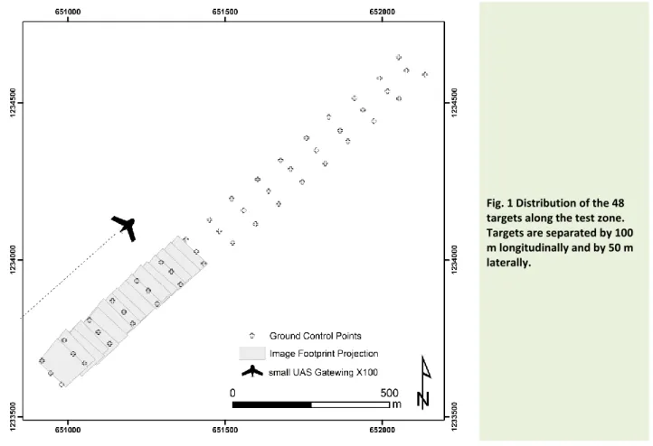
The study was carried out in southern Burkina Faso in the Nazinga Game Ranch (NGR), which covers about 940 km² along the border with Ghana. Vegetation cover is composed of a mosaic of clear shrubs, woody savannah and tree savannah. Apart from the micro-relief of the tree canopy, the terrain relief shows a negligible variation in altitude.

Fig. 1 Distribution of the 48 targets along the test zone. Targets are separated by 100 m longitudinally and by 50 m laterally.

The test strip used in this study is a transect of 1.5 km long oriented SW-NE. The width of the strip relies on the flight altitude (Equation 1). Three different flight heights were tested: 100 m, 150 m and 200 m, corresponding to an image swath of respectively 123 m, 184 m and 246 m. Low altitude flights are more appropriate because they enable easier animal detectability [7]. In order to easily define Ground Control Points (GCPs) with accurate global coordinates, a set of 48 targets was arranged at regular intervals on a grid measuring 100 meters along by 50 meters apart from the transect (Figure 1). The coordinates of each target were measured with a sub-metric SxBLUE II GPS (http://www.sxbluegps.com). Theoretical image overlap was set to 90%, but due to wind, effective overlap was highly variable (ranges from 60% to 90% in average per sampling strip). A total of five flights were carried out over two half-days (15/02/2012 PM and 16/02/2012 AM): 3 flights at 100 m AGL, one at 150 m AGL and one at 200 m AGL. 16th February was the windier of the two days, with a wind speed of 3 Beaufort (12-19 km/h). For each flight, the drone twice went over the strip transect (return), providing 2 strips per flight. A quick visual evaluation of the 10 sets of images led us to discard two of them, because the image overlap was insufficient to carry out an aerotriangulation process. The 8 sets of images that were ultimately analyzed are described in Table 1.

Processing of images and estimation of surface area

Images acquired with an aerial platform need to be georeferenced in order to use them for quantitative purposes such as the calculation of surface area or density [33,40]. Among the different ways to implement georeferencing, a distinction needs to be made between direct and indirect georeferencing. Indirect georeferencing requires the definition of GCPs corresponding to identifiable features in the imagery for which the coordinates are known. This task is time consuming [41], and even sometimes infeasible due to a lack of clearly identifiable GCPs on large scale images [33]. Direct georeferencing takes advantage of both the position (X0, Y0, Z0) and the orientation (omega, phi, kappa) of the camera, provided by integrated GPS/IMU [19,42]. Nevertheless, the implementation of direct georeferencing in the case of a UAS is somewhat challenging, due to the limited accuracy of the GPS and inertial measurement units involved [13,40]. The georeferencing method should be considered on the basis of the requirements of the mapping project [40]. For wildlife surveys, the requirements in terms of georeferencing accuracy are low, as the density is calculated on the basis of the total surface area of the sampling strips. UAS images may be georeferenced either by assigning individually low accurate Exterior Orientation (acronym: EO, which is position & orientation) from the GPS/IMU system or by using a Structure from Motion technique [38] for refining the EO of the block of imagery [13,42]. Taking into account the fact that (i) the desired information (total surface area of the strip) does not necessary require a high level of geometric accuracy at the single image level and that (ii) strips can be made up of a very high number of pictures, three methods presenting a graduated level of complexity and potential accuracy were compared.

1. Image footprint projection - IFP

In the IFP method, the position and altitude of the camera, logged during the flight, are used to compute a simple projection of the images on a horizontal plane corresponding to the ground level (Figure 2). This method uses collinearity equations, which describe the relationship between a three-dimensional object and its projection onto a two-three-dimensional image [39], in order to transform the frame of an image from its internal coordinate system to a polygon drawn within a geographical coordinate system [19,43]. Each of the 4 corners of each camera frame is projected by means of Equation 2 and these sets of corners are subsequently linked together. A real example of the IFP method is provided in appendix 1. All the polygons corresponding to individual images are then merged and the strip surface area equals that of the resulting polygon. In this study, the earth-based coordinate system utilized was the projection system Universal Transverse Mercator 30N.

𝑋 = −𝐻_𝑓 𝑚11𝑥+𝑚21𝑦−𝑚31𝑓

𝑚13𝑥+𝑚23𝑦−𝑚33𝑓+ 𝑋0 Eq. 2

𝑌 = −𝐻_𝑓 𝑚12𝑥+𝑚22𝑦−𝑚32𝑓 𝑚13𝑥+𝑚23𝑦−𝑚33𝑓 + 𝑌0

Where X,Y are the earth-based coordinates [m], x, y are the camera frame coordinates [mm],

f is the camera focal length,

𝐻_𝑓 is the flight altitude Above Ground Level (AGL) [m], 𝑋₀ and 𝑌₀ are the position of the camera (optical center) [m],

𝑚_𝑖𝑖 are the 9 coefficients of the rotation matrix, computed from the orientation of the drone (roll, pitch, yaw)

Figure 2 Illustration of Image Footprint Projection (IFP). This georeferencing method uses direct georeferencing. Figure adapted from Sugiura et al. [19].

2. Bundle block adjustment without GCP (direct georeferencing) - BBA DG

Recent developments in automatic image matching have led to the release of low-cost and versatile software, taking advantage of both photogrammetric and computer vision (Structure from Motion; SfM) techniques. Although a review of SfM is not appropriate for this paper, we will give an overall insight into its tenets and describe briefly the reasons why this approach is particularly suited to UAS imagery. Images acquired by UAS are fundamentally different from those collected by traditional aerial platforms [13]. These images are characterized by a low-oblique vantage points, and a high angular variation between successive images [36]. Furthermore, the low altitude of the platform causes important perspective distortions [13]. These UAS images are also often marred by a high variation in illumination and by occlusions [42]. Another difference lies in the sensor: UAS platforms make use of consumer grade cameras, which were not initially designed for metric purposes, and which have a high (and unknown) level of distortion and low geometric stability [44]. On the other hand, traditional aerial platforms use metric cameras, which are stable, and have a larger charged couple device and a known

level of distortion [45]. Moreover, the number of images is appreciably greater when using UAS as a mapping tool, contrary to traditional aerial platforms. SfM was designed to restitute the 3D relief of an object from a randomly acquired image dataset. The process of dense-matching may be interpreted as a three step workflow: first of all, automatic generation of image tie points is performed, based on image feature descriptors and matching algorithms, such as the scale invariant feature transform [46]. Secondly, the aerotriangulation model is computed by means of a bundle block adjustment (BBA). The aerotriangulation model is the 3D position of each tie point as well as the external orientation and the inner parameters of the camera for each image from the block. We refer the reader to Triggs et al. [47] for an explanation of BBA. The sparse 3D model may then be georeferenced. Thirdly, a dense-matching algorithm determines the geometry and the position of the object. The dense 3D model is used for orthorectifying individual images in order to remove distortions regarding perspective and relief. The SfM photogrammetric software used in this study was the Agisoft PhotoscanTM _{LLC 0.90. With this} software, images are oriented with a self-calibrating-BBA algorithm and relief is computed by multi-view dense-matching. The tool "Optimization" of this software has been used to avoid non-linear distortions [48]. In the present study, the photoscan parameters were set to medium quality for image alignment and geometry building.

In the BBA DG approach, model georeferencing is performed using the external orientation from the navigation files. Approximate values of camera pose are extracted from the navigation files and serve for the georeferencing of the image block. Images are orthorectified and assembled in an orthophotomosaic whose contour is then converted into a polygon. The surface area of the strip is then calculated as the surface area of this resulting polygon.

3. Absolute orientation of images using GCPs (indirect georeferencing) - BBA IG

This method uses the same workflow as the BBA DG approach, except for the georeferencing. With BBA IG, GCPs are used instead of the EO to transform the relative orientation in an absolute reference frame. The use of GCPs improves the georeferencing of the resulting orthophotomosaic in comparison to the use of exterior orientation, as the level of accuracy of GCPs position outperforms the accuracy of EO position. The effort needed to set and georeference the targets along the strips makes it unlikely that this method will be reproduced for wider studies. This method is used to produce a surface area estimation, which can be considered as the reference, due to the numerous GCPs and their high position accuracy. Processing were performed using Photoscan.

Comparison of surface area estimation techniques

The BBA IG method was considered as the reference, and was used to compute the relative error (bias) for each surface area estimation made using the first two methods. These performance metrics were then compared using a two-way ANCOVA (i. e. a general linear model with one quantitative factor and one qualitative factor), the method of surface area estimation being considered as a factor, and the elevation as a co-variate.

Processing was timed for each method in order to provide a comparison. This test was performed by an experienced user on strip n°1 (see Table 1) on a laptop (16 GB ram, i7 core 2.00 GHz). Computation-time is strongly dependent on computer performance and on the resolution used for dense-matching.

Results

Results of strip surface area computation are presented in Table 1 and an illustration of the workflow for acquiring and processing UAS images is shown on Figure 3. The relative bias of the IFP and BBA DG methods was computed as the difference compared to the reference surface area (BBA IG). The

maximal difference was +4.7% for IFP and -7.2% for BBA DG. Two-way ANCOVA analysis showed that the type of method had a significant influence on the relative error (p-value = 0.0064). BBA DG resulted in a underestimation of -2.3%, whereas the IFP method caused an overestimation of 1.4%. One sample t-test demonstrated that IFP was not significantly different from BBA IG (p-value = 0.142). However, BBA DG showed a significant bias (p-value = 0.039). Nevertheless, the mean relative error of both methods can be regarded as relatively low considering the range of variability commonly encountered in wildlife surveys. Neither the flight height nor the interaction between flight height and the calculating method showed a significant impact on the accuracy of the surface area estimation (p-value of 0.08 and 0.8 respectively). It is interesting to note that in this case study, despite the fact that BBA DG takes into account the relief of the scene, this method demonstrated a lower level of accuracy in comparison with the IFP method. One might expect that in the case of a more pronounced relief, BBA DG will show a clear superiority over the IFP method.

The IFP method takes 9 minutes to process, BBA DG 23 minutes and BBA IG 45 minutes for one single strip. BBA DG requires much more time than IFP due to the computation time needed for image matching. On the other hand, BBA IG is very time-consuming because the user has to manually mark each GCP on the different images. This trend in implementation time highlights the gradient of complexity of the three methods. Whereas the IFP method can be easily implemented in any GIS software and is not demanding in terms of image quality, BBA (DG and IG) relies on the SfM software solution, which requires computer power. Moreover, IFP accommodates aerial images with a low level of overlap or even without any overlap. BBA is applicable only if the image overlap enables an automatic image matching. This is difficult if the images are blurred, where objects such as animals or shadows have moved between two images.

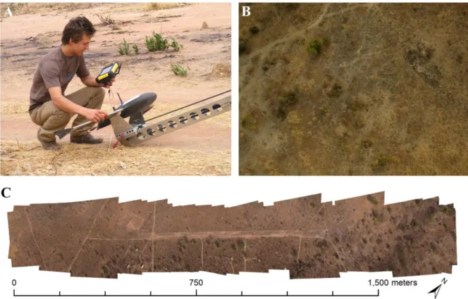
Fig. 3 Creation of the orthophotomosaic for the determination of the surface area of sampling strip. A) The lightweight UAS Gatewing X100 on the catapult launcher, ready for departure. B) One of the raw aerial image (flight altitude: 200 meters above ground level). C) Orthophotomosaic of the test field generated tanks to Structure from Motion techniques.

Table 1 Characteristics of the 8 aerial strips and the strip surface area estimated using the three methods. BBA IG (Bundle Block Adjustment with Indirect Georeferencing) is the reference. IFP (Individual Footprint Projection) generally gives a lower bias than BBA DG (Bundle Block Adjustment with Direct Georeferencing).

Strip ID Flight ID Number of Images Flight altitude [m] Overlap [%]

Surface area estimation (ha) Relative error (%) BBA IG IFP BBA DG IFP BBA DG

1 1 51 100 69 22.3 21.9 20.7 -1.9 -7.2 2 1 65 100 76 21.8 22.3 21.6 2.4 -0.6 3 2 108 100 84 23.7 23.5 23.6 -1.2 -0.4 4 3 99 100 83 23.1 22.9 22.9 -0.7 -0.7 5 4 54 150 79 35.4 36.3 33.9 2.5 -4.3 6 4 69 150 84 34.7 35.7 33.5 2.8 -3.6 7 5 46 200 79 53.8 56.3 52.9 4.7 -1.6 8 5 92 200 89 54.4 55.7 54.5 2.4 0.2 Mean error: +1.4 -2.3 Residual mean square error: 2.57 3.29 P-Value: 0.142 0.039

Discussion

For the purpose of wildlife surveys with UAS, the surface area computation needs to be sufficiently accurate but it also needs to be quick and easily manageable. Individual Footprint Projection (IFP) appears to outperform the method of BBA with Direct Georeferencing, due to its higher accuracy (RMSE of 2.57% for IFP and 3.29% for BBA DG), its quicker processing time and its relatively low complexity, enabling its implementation in most types of commonly existing GIS software. This direct georeferencing technique also presents the advantage of being insensitive to variations in overlap between pictures within a flight line. However it still remains important to maintain this overlap as it is a primary factor during the counting phase [7]. Of course, aligning the images together has many advantages and shows great potential for high temporal and spatial resolution mapping, but the use of this approach for surface area computation appears to be excessively demanding in terms of human and computer work.

An in-house software program has been developed in order to implement the collinearity equation so as to project image footprints based on X100 telemetry information and on the camera specification (focal length and sensor size). One of the major drawbacks of the IFP method is that it does not account for the topography of the area under study. The good performance of the IFP method in this study relates to the very flat relief of the study area. Indeed, IFP is based on the assumptions that the terrain is flat, the flight height is constant and the telemetry data (GPS position and gyro angles) are correct. Although this type of unrelieved landscape is very representative of the areas usually inventoried in western Africa, we recommend estimating the sensitivity of the IFP method at an accentuation of the relief. Under these conditions, the use of a global digital ground model such as shuttle radar topography mission (SRTM) would probably limit the number of errors linked to the variations in height within strip samples.

The use of small UASs in big mammal surveys opens up interesting perspectives. Up to now, no other investigations had shown an interest in the sampling strip area estimation. Most of the studies have demonstrated the detection possibilities of various animals, ranging from flocks of waterbirds to middle and large-sized species such as deers, bisons, elephants or bears, as well as the possibilities of

counting them with accuracy [6,7,12,26,27,30,49]. Wilkinson [6] also tested methods to assemble and georeference the images with the aim of obtaining quality mosaics to easily spot and count animals. These interesting first steps are probably enough to assess the number of animals in a group or in a population with a well-known range. However, the issue is different for many species, particularly in tropical areas. Most live in groups spread over very large areas, which makes it impossible to take them all into account. Inventories by sampling is the usual method used to estimate the population densities required for the management of those areas. This study demonstrates the existence of a quick, easy and accurate way of estimating the sampling strip area, thus offering the possibility of aerial inventories with UAS.

In future research, it would be interesting to investigate the use of the various sampling modalities in order to cover in a coherent and effective way the wide areas that are usually the object of wildlife surveys. It is unlikely that small drones with a relatively low endurance, such as the X100, could be adapted for use in the systematic transects system classically implemented with piloted surveys. It is therefore necessary to apply adaptations to the sampling plan and to find technical solutions in order to improve the autonomy of UASs.

Implications for conservation

The use of small UASs in big mammal surveys is in its infancy, but it opens up very promising perspectives. The detection and counting of large-sized species has already been investigated and is considered as a viable alternative to traditional aerial survey. This research concludes that the computation of the sampling strip surface area, a vital piece of information for density computation, requires no more than the position and altitude delivered by the onboard GPS/IMU, which can be advantageously used for individual image footprint projection. Although photogrammetry and SfM techniques are of great interest for mapping tropical ecosystems, the unmanned aerial surveys of wildlife do not require the use of such an approach in order to deliver an estimation of the sampling strip surface area.

Acknowledgements

The authors would like to acknowledge the Office National des Aires Protégées (OFINAP) and the Nazinga Game Ranch authority for their hospitality during the study. Acknowledgements also go to Géraldine Le Mire, Peter Hotton and Phillis Smith for their correction and advice on the paper’s written English. The assistance provided by Gatewing support is greatly appreciated. This research was funded by the Department of Forest, Nature and Landscape at the University of Liège Gembloux Agro-Bio Tech.

References

[1] Jachmann, H. 2001. Estimating abundance of African wildlife: an aid to adaptive management, Kluwer Academic Publishers, Boston.

[2] Jachmann, H. 2008. Evaluation of four survey methods for estimating elephant densities. African Journal of Ecology 29:188–195.

[3] Norton-Griffiths, M. 1978. Counting animals, African Wildlife Leadership Foundation, Nairobi, Kenya.

[4] Bouché, P., Lejeune, P. and Vermeulen, C. 2012. How to count elephants in West African savannahs? Synthesis and comparison of main gamecount methods. BASE 16:77–91.

[5] Watts, A. C., Perry, J. H., Smith, S. E., Burgess, M. A., Wilkinson, B. E., Szantoi, Z., Ifju, P. G. and Percival, H. F. 2010. Small Unmanned Aircraft Systems for Low-Altitude Aerial Surveys. The Journal of Wildlife Management 74:1614–1619.

[6] Wilkinson, B. E. 2007. The design of georeferencing techniques for an unmanned autonomous aerial vehicle for use with wildlife inventory surveys: A case study of the National Bison Range, Montana., M.S. thesis, University of Florida, Florida.

[7] Vermeulen, C., Lejeune, P., Lisein, J., Sawadogo, P. and Bouché, P. 2013. Unmanned Aerial Survey of Elephants. PLoS ONE 8:e54700.

[8] Dunham, K. M. 2012. Trends in populations of elephant and other large herbivores in Gonarezhou National Park, Zimbabwe, as revealed by sample aerial surveys. Afr. J. Ecol.

[9] Ferreira, S. M. and Aarde, R. J. 2009. Aerial survey intensity as a determinant of estimates of African elephant population sizes and trends. South African Journal of Wildlife Research 39:181–191. [10] Bouché, P., Douglas-Hamilton, I., Wittemyer, G., Nianogo, A. J., Doucet, J.-L., Lejeune, P. and

Vermeulen, C. 2011. Will Elephants Soon Disappear from West African Savannahs? PLoS ONE

6:e20619.

[11] Dunford, R., Michel, K., Gagnage, M., Piegay, H. and Tremelo, M. L. 2009. Potential and constraints of Unmanned Aerial Vehicle technology for the characterization of Mediterranean riparian forest. International Journal of Remote Sensing 30:4915–4935.

[12] Martin,, J., Edwards,, H. H., Burgess,, M. A., Percival,, H. F., Fagan,, D. E., Gardner,, B. E., Ortega-Ortiz,, J. G., Ifju,, P. G., Evers,, B. S. and Rambo,, T. J. 2012. Estimating Distribution of Hidden Objects with Drones: From Tennis Balls to Manatees. PLoS ONE 7:e38882.

[13] Turner, D., Lucieer, A. and Watson, C. 2012. An Automated Technique for Generating Georectified Mosaics from Ultra-High Resolution Unmanned Aerial Vehicle (UAV) Imagery, Based on Structure from Motion (SfM) Point Clouds. Remote Sensing 4:1392–1410.

[14] Finn, R. L. and Wright, D. 2012. Unmanned aircraft systems: Surveillance, ethics and privacy in civil applications. Computer Law and Security Review 28:184–194.

[15] Eisenbeiss, H. 2009. UAV photogrammetry, ETH, Zurich.

[16] Haarbrink, R. and Koers, E. 2006. Helicopter UAV for photogrammetry and rapid response. In 2nd Int. Workshop“ The Future of Remote Sensing”, ISPRS Inter-Commission Working Group I/V Autonomous Navigation, p 1.

[17] Hunt, E. R., Hively, W. D., Fujikawa, S. J., Linden, D. S., Daughtry, C. S. T. and McCarty, G. W. 2010. Acquisition of NIR-Green-Blue Digital Photographs from Unmanned Aircraft for Crop Monitoring. Remote Sensing 2:290–305.

[18] Lelong, C. C. D., Burger, P., Jubelin, G., Roux, B., Labbé©, S. and Baret, F. 2008. Assessment of unmanned aerial vehicles imagery for quantitative monitoring of wheat crop in small plots. Sensors

8:3557–3585.

[19] Sugiura, R., Noguchi, N. and Ishii, K. 2005. Remote-sensing Technology for Vegetation Monitoring using an Unmanned Helicopter. Biosystems Engineering 90:369 – 379.

[20] Niethammer, U., James, M. R., Rothmund, S., Travelletti, J. and Joswig, M. 2012. UAV-based remote sensing of the Super-Sauze landslide: Evaluation and results. Engineering Geology 128:2– 11.

[21] Westoby, M. J., Brasington, J., Glasser, N. F., Hambrey, M. J. and Reynolds, J. M. 2012. “Structure-from-Motion”photogrammetry: A low-cost, effective tool for geoscience applications. Geomorphology.

[22] Verhoeven, G., Doneus, M., Briese, C., Vermeulen, F. 2012. Mapping by matching: A computer vision-based approach to fast and accurate georeferencing of archaeological aerial photographs. Journal of Archaeological Science 39:2060–2070.

[23] Getzin, S., Wiegand, K. and Schöning, I. 2012. Assessing biodiversity in forests using very high-resolution images and unmanned aerial vehicles. Methods in Ecology and Evolution 3:397–404. [24] Hardin, P. J. and Hardin, T. J. 2010. Small Scale Remotely Piloted Vehicles in Environmental

Research. Geography Compass 4:1297–1311.

[25] Lejot, J., Delacourt, C., Piégay, H., Fournier, T., Trémélo, M.-L. and Allemand, P. 2007. Very high spatial resolution imagery for channel bathymetry and topography from an unmanned mapping controlled platform. Earth Surface Processes and Landforms 32:1705–1725.

[26] Israel, M. 2011. A UAV-based roe deer fawn detection system. International Archives of the Photogrammetry, Remote Sensing and Spatial Information Sciences XXXVIII-1.

[27] Jones, G. P., Pearlstine, L. G. and Percival, H. F. 2006. An assessment of small unmanned aerial vehicles for wildlife research. Wildlife Society Bulletin 34:750–758.

[28] Koski, W. R., Allen, T., Ireland, D., Buck, G., Smith, P. R., Macrender, A. M., Halick, M. A., Rushing, C., Sliwa, D. J. and McDonald, T. L. 2009. Evaluation of an unmanned airborne system for monitoring marine mammals. Aquatic Mammals 35:347–357.

[29] Chabot, D. and Bird, D. M. 2012. Evaluation of an off-the-shelf Unmanned Aircraft System for Surveying Flocks of Geese. Waterbirds 35:170–174.

[30] Sarda-Palomera, F., Bota, G., Vińolo, C., Pallarés, O., Sazatornil, V., Brotons, L., Gomáriz, S. and Sardŕ, F. 2012. Fine-scale bird monitoring from light unmanned aircraft systems. Ibis 154:177–183. [31] Koh, L. P. and Wich, S. A. 2012. Dawn of drone ecology: low-cost autonomous aerial vehicles for

conservation. Tropical Conservation Science 5:121–132.

[32] Anderson, K. and Gaston, K. J. 2013. Lightweight unmanned aerial vehicles will revolutionize spatial ecology. Frontiers in Ecology and the Environment.

[33] Xiang, H. and Tian, L. 2011. Development of a low-cost agricultural remote sensing system based on an autonomous unmanned aerial vehicle (UAV). Biosystems Engineering.

[34] Berni, J., Zarco-Tejada, P., Surez, L., González-Dugo, V. and Fereres, E. 2008. Remote sensing of vegetation from uav platforms using lightweight multispectral and thermal imaging sensors. The International Archives of the Photogrammetry, Remote Sensing and Spatial Information Sciences, XXXVII.

[35] Harwin, S. and Lucieer, A. 2012. Assessing the accuracy of georeferenced point clouds produced via multi-view stereopsis from Unmanned Aerial Vehicle (UAV) imagery. Remote Sensing 4:1573– 1599.

[36] Zhang, Y., Xiong, J. and Hao, L. 2011. Photogrammetric processing of low-altitude images acquired by unpiloted aerial vehicles. The Photogrammetric Record 26:190–211.

[37] Watts, A. C., Ambrosia, V. G. and Hinkley, E. A. 2012. Unmanned Aircraft Systems in Remote Sensing and Scientific Research: Classification and Considerations of Use. Remote Sensing 4:1671– 1692.

[38] Snavely, N., Seitz, S. M. and Szeliski, R. 2008. Modeling the World from Internet Photo Collections. International Journal of Computer Vision 80:189–210.

[39] Wolf, P. R. and Dewitt, B. A. 2000. Elements of Photogrammetry: with applications in GIS, McGraw-Hill New York, NY, USA.

[40] Perry, J. H. 2009. A synthesized directly georeferenced remote sensing technique for small unmanned aerial vehicles, M.S. thesis, University of Florida.

[41] Moran, M. S., Inoue, Y. and Barnes, E. 1997. Opportunities and limitations for image-based remote sensing in precision crop management. Remote Sensing of Environment 61:319–346.

[42] Barazzetti, L., Remondino, F. and Scaioni, M. 2010. Automation in 3D reconstruction: Results on different kinds of close-range blocks. In ISPRS Commission V Symposium Int. Archives of Photogrammetry, Remote Sensing and Spatial Information Sciences, Newcastle upon Tyne, UK. [43] Cramer, M., Stallmann, D. and Haala, N. 2000. Direct Georeferencing Using Gps/inertial Exterior

Orientations For Photogrammetric Applications. International Archives of Photogrammetry and Remote Sensing 198–205.

[44] Läbe, T. and Förstner, W. 2004. Geometric stability of low-cost digital consumer cameras. In Proceedings of the 20th ISPRS Congress, Istanbul, Turkey, pp 528–535.

[45] Sanz-Ablanedo, E., Rodriguez-Pérez, J. R., Armesto, J. and Taboada, M. F. A•. 2010. Geometric Stability and Lens Decentering in Compact Digital Cameras. Sensors 10:1553–1572.

[46] Lowe, D. G. 2004. Distinctive image features from scale-invariant keypoints. International journal of computer vision 60:91–110.

[47] Triggs, B., McLauchlan, P., Hartley, R. and Fitzgibbon, A. 2000. Bundle adjustment—a modern synthesis. Vision algorithms: theory and practice 153–177.

[48] Fonstad, M. A., Dietrich, J. T., Courville, B. C., Jensen, J. L. and Carbonneau, P. E. 2013. Topographic structure from motion: a new development in photogrammetric measurement. Earth Surface Processes and Landforms 38:421–430.

[49] Chabot, D. 2009. Systematic evaluation of a stock unmanned aerial vehicle (UAV) system for small-scale wildlife survey applications, M.S. thesis, Mcgill University, Montreal, Quebec, Canada.

Appendix 1: Image Footprint Projection - an example. The input data are the telemetry data and the

sensor specifications. The result is the projected coordinates of the four corners of the image footprint.

Exterior orientation of the image

Image name R0020216.JPG X0 latitude [degree] -1.618321541 Y0 longitude [degree] 11.15593834 Z0 [m] 379.088 Kappa [degree] 50.5 Omega [degree] 4.3 Phi [degree] 0.3 Flight altitude (H) [m] 100

Projection of the X0 and Y0 in the Coordinate System UTM 30 Nord

X0 [m] 650873.590857522

X0 [m] 1233573.71612906

Interior orientation of the camera RICOH GRIII :

Sensor length [m] (Ls) 0.0076

Sensor heigth (Hs) 0.0057 Focal lenght (f) 0.00617

Coordinate of the four corners of the sensor in the image coordinate system

Corner up right x1 = Ls / 2 y1 = Hs / 2 Corner up left x2 = -Ls / 2 y2 = Hs / 2 Corner down left x3 = -Ls / 2 y3 = -Hs / 2 Corner down right x4 = Ls / 2

y4 = -Hs / 2

Rotational matrix to transform the image coordinate system to world coordinate system (e.g. UTM 30 N)

m11 = Cosinus(phi) * Cosinus(kappa) m12 = -Cosinus(phi) * Sinus(kappa) m13 = Sinus(phi)

m21 = Cosinus(omega) * Sinus(kappa) + Sinus(omega) * Sinus(phi) * Cosinus(kappa) m22 = Cosinus(omega) * Cosinus(kappa) - Sinus(omega) * Sinus(phi) * Sinus(kappa) m23 = -Sinus(omega) * Cosinus(phi)

m31 = Sinus(omega) * Sinus(kappa) - Cosinus(omega) * Sinus(phi) * Cosinus(kappa) m32 = Sinus(omega) * Cosinus(kappa) + Cosinus(omega) * Sinus(phi) * Sinus(kappa) m33 = Cosinus(omega) * Cosinus(phi)

The collinearity equations

Project the 4 corners of the sensor in the world coordinate system

Y1 = -H * ((m12 * x1 + m22 * y1 - m32 * f) / (m13 * x1 + m23 * y1 - m33 * f)) + Y0 X2 = -H * ((m11 * x2 + m21 * y2 - m31 * f) / (m13 * x2 + m23 * y2 - m33 * f)) + X0 Y2 = -H * ((m12 * x2 + m22 * y2 - m32 * f) / (m13 * x2 + m23 * y2 - m33 * f)) + Y0 X3 = -H * ((m11 * x3 + m21 * y3 - m31 * f) / (m13 * x3 + m23 * y3 - m33 * f)) + X0 Y3 = -H * ((m12 * x3 + m22 * y3 - m32 * f) / (m13 * x3 + m23 * y3 - m33 * f)) + Y0 X4 = -H * ((m11 * x4 + m21 * y4 - m31 * f) / (m13 * x4 + m23 * y4 - m33 * f)) + X0 Y4 = -H * ((m12 * x4 + m22 * y4 - m32 * f) / (m13 * x4 + m23 * y4 - m33 * f)) + Y0

The image footprint projection of image “R0020216.JPG” is the polygon delimited by the four corners (X1, Y1), (X2, Y2), (X3, Y3) and (X4, Y4), either (650941,1233551), (650865, 1233643), (650791,