Centre de Recherche en économie de l’Environnement, de l’Agroalimentaire, des Transports et de l’Énergie
Center for Research on the economics of the Environment, Agri-food, Transports and Energy
_______________________
Abbassi : Corresponding author. Assistant Professor, Faculty of Economics and Management of Nabeul, University of Carthage, Tunisia and Center for Research on the Economics of the Environment, Agri-food, Transports and Energy (CREATE)
Tamini : Assistant Professor, Laval University, Department of Agricultural Economics and Consumer Science, CREATE and Egg Industry Economic Research Chair
Dakhlaoui : Professor, Industrial Economics Department in Tunisia Polytechnic School, LEGI, Faculty of Economics and Management of Nabeul, University of Carthage, Tunisia
Les cahiers de recherche du CREATE ne font pas l’objet d’un processus d’évaluation par les pairs/CREATE working papers do not undergo a peer review process.
ISSN 1927-5544
Production Cost Asymmetry, Minimum Access and
Reciprocal Dumping
Abdessalem Abbassi
Lota D. Tamini
Ahlem Dakhlaoui
Cahier de recherche/Working Paper 2013-7
Abstract:
In this article we propose a bilateral dumping model in which the minimum access level is endogenous. Regions compete with one another using Cournot conjectures and engage in interregional dumping as in Brander and Krugman’s (1983) reciprocal dumping model. International trade is hindered by restrictive Tariff rate Quota (TRQs). The model features two regions and one product. We derive the conditions under which it is optimal to observe interregional trade and those under which trade does not exist. The results show that the world price and the difference in production costs between regions play an important role in determining whether bilateral trade exists. In the presence of bilateral trade, the region with the largest market size will obtain the largest share of import volumes permitted under the minimum access system while in the absence of interregional trade, the distribution of import permits between regions will also depends on the product cost asymmetry. When only the most efficient region exports to the least efficient region, production costs asymmetry, transaction costs and world price level determine whether the smaller or larger region obtains the larger share of product import allowed under minimum access commitment. In all cases, we show that in a country like Canada, creation of “artificial barriers” to interprovincial trade of products under supply management system lowers the welfare of at least one of the regions, along with the global welfare.
Keywords: Minimum access, reciprocal dumping, cost asymmetry Résumé:
Dans cet article, nous proposons un modèle de dumping bilatéral avec un niveau d'accès minimum endogène. Les régions se concurrencent entre elles en utilisant des conjectures à la Cournot et pratiquent du dumping interrégional selon le modèle de dumping réciproque de Brander et Krugman (1983). Le commerce international est entravé par des contingents tarifaires. Le modèle comporte deux régions et un produit. Nous dérivons les conditions pour lesquelles il est optimal d’observer des échanges interrégionaux et celles pour lesquelles le commerce n'existe pas. Les résultats obtenus montrent que le prix mondial et de la différence des coûts de production entre les régions jouent un rôle important dans l’existence ou non du commerce bilatéral. En présence de commerce bilatéral, la région ayant le marché le plus important aura les parts les plus importantes de l’accès minimum tandis qu’en l’absence de commerce interrégional, les affectations de l’accès minimum dépendront également du paramètre de coût. Lorsque seule la région la plus efficace exporte vers la région la moins efficace, l’asymétrie des coûts de production, les coûts de transaction et le prix mondial déterminent si la plus grande part des importations de produits autorisés en vertu de l'engagement d'accès minimum va ou non à la région la plus peuplée. Dans tous les cas, nous montrons que dans un pays comme le Canada, la mise en place de «barrières artificielles» au commerce interprovincial des produits relevant du système de gestion de l'offre diminue le bien-être d'au moins l'une des régions et le bien-être global.
Mots clés: Accès minimum, dumping réciproque, asymétrie des coûts Classification JEL: F120, Q170, R120
Production cost asymmetry, minimum access and reciprocal dumping
1 Introduction
Under the Uruguay Accord, non-tariff barriers (quotas) have been converted into tariff barriers in the agri-food sector. To ensure that tariffs are not completely protectionist, World Trade Organization (WTO) member nations have created a system of tariff rate quotas (TRQs) which is a combination of tariffs and quotas. A small quantity of a product (minimum access) can be imported at a minimum tariff (intra-quota tariff), whereas imports that exceed the quantity permitted by minimum access to the market are subject to a higher, often prohibitive tariff. For example, Canada protects its markets from import competition in the egg, poultry and dairy sectors by imposing a minimum tariff on foreign imports as long as they are less than or equal to the commitments made under the North American Free Trade Agreement (NAFTA) and WTO.1 Beyond this level, imports are subject to much higher tariffs (for example up to 230% for chicken). In its latest evaluation of the European Union trade policy, the WTO reported that in 2010, the European Union had notified 112 tariff rate quotas in the agricultural sector, 34 of which were totally used, and 10 used between 80% and 99% (WTO, 2013). In the United States, this mechanism prevails in the dairy2 and sugar3 sectors. Several other countries use such instruments, which justifies the will of some WTO member nations to reduce extreme tariffs and/or increase minimum access. Higher tariffs should be reduced in a larger proportion than lower tariffs. However, the revised draft modalities of July 2008 recognizes the concept of
1
See the website of Foreign Affairs, Trade and Development Canada at http://www.international.gc.ca/controls-controles/prod/agri/index.aspx?menu_id=3. Accessed September 4, 2013.
2 See the USDA website at: http://www.fas.usda.gov/itp/imports/usdairy.asp . Accessed September 4, 2013. 3 See the USDA website at http://www.fas.usda.gov/itp/imports/ussugar.asp. Accessed September 4, 2013.
sensitive products,4 for which countries are not obliged to apply negotiated tariff reductions. Minimum access should then be increased to compensate for the lesser reduction of tariffs.5 The study of the consequences of an increase in minimum access and therefore levels of optimality in terms of producer surplus, consumer surplus and global welfare is therefore pertinent.
The prevalence of import quotas in several countries and various economic sectors6 has spawned rich literature on this question, including recent works by Chao and Yu (1991), Feenstra (1995), Maggie and Rodriguez-Clare (2000), Kreickmeier (2005) and Chao et al. (2010). In the agri-food sector specifically, several studies have analyzed the impact of import quotas on a country's welfare using modeling approaches of varying complexity. Gervais and Lapan (2001) perform a dynamic analysis of the effects of tariff rate quotas, whereas Gervais and Lapan (2002) introduce uncertainty in their model. Pouliot and Larue (2012) consider the segments of production, processing and retail. These authors show that an increase in TRQs defined as a fraction of internal production can lead to an increase in retailers’ internal prices if the price of imports is between the unit production cost and firms’ internal price upstream. Larue, Gervais and Pouliot (2008) analyze a situation in which local production is controlled by a monopoly (e.g. agricultural marketing board) with the possibility of restricting local producers’ supply. The authors show that at high price levels, the increase in minimum access commitments is the preferred trade policy option.
4 See the WTO website at http://www.wto.org/english/tratop_e/dda_e/meet08_e.htm . Accessed September 4, 2013. 5 See draft text at http://www.wto.org/english/tratop_e/agric_e/chair_texts08_e.htm. Accessed September 3, 2013. 6
See WTO site at http://tariffanalysis.wto.org/report/TariffQuotas.aspx for the agricultural sector. This situation was also observed in other economic sectors. Deardorff and Stern (1999, tables 3.1 and 3.2) report that in 1993, in the United States all non-tariff barriers and quotas (as measured by frequency ratios) were 22.9% and 18.1% respectively, for all products. The corresponding figures for the European Union were 23.7% and 17.2%.
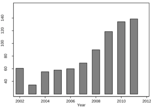
In both Canada and the European Union, import management involves not only allocating imports under minimum access to different provinces/countries, but also controlling production to guarantee a sufficiently high domestic price. National production is allocated to different regions/countries, each of which should source mainly on its local market. In Canada, supply management bodies have thus been put in place to ensure effective allocation of production quotas between provinces and avoid interprovincial “trade wars.”7 However, data on interprovincial trade of products under supply management indicate that this trade is generally increasing. Figures 1.a and 1.b present, respectively, the evolution of Canadian interprovincial trade in the shell egg and live chicken sectors.
Ideally, production quotas should be distributed to minimize production and transaction costs, in order to satisfy the demand of consumers in different regional markets. Using game theory, Larue and Lambert (2012) explain why Canadian producers and processors engage in interprovincial trade at the risk of attracting legislators’ attention, and paradoxically, ultimately lowering their profit. Businesses operate outside of their province even if they are likely to earn a lower profit than if they stayed in their respective province. Bayliss and Furtan (2003) use data on Canadian dairy production to show that provinces do not cooperate even in cases where there is a mutual interest, as in the case of lobbying the federal government to put trade barriers in place. Furtan, Sauer and Jensen (2009) observe a similar situation for European Common agricultural policy. In both Canada and the European Union, the situation is therefore similar to
7 For example, Chicken Farmers of Canada (CFC) is in charge of administering the national production system. CFC determines the national production level and distributes this production to the provinces based on requests it receives from provincial trade boards. The Canadian Broiler Hatching Egg Marketing Agency (CBHEMA), Egg Farmers of Canada (EFC) and Turkey Farmers of Canada (TFC) are the national bodies that govern their respective sectors at the national level. The Canadian Dairy Commission (CDC) sets support prices for butter and milk powder and chairs the Canadian Milk Supply Management Committee (CMSMC), which sets the national objective for milk production under the National Milk Marketing Plan. See the Canadian Justice Department website for the Farm Products Agencies Act. http://lois-laws.justice.gc.ca/eng/acts/F-4/ / Accessed February 18, 2013.
bilateral dumping model as proposed by Brander and Krugman (1983), in which trade can exist even in the absence of a comparative advantage of either country8; the gains exceed the additional transport costs. In this type of model, it is impossible to determine a priori the net gain in terms of welfare for a situation in which various regions (or countries) engage in bilateral dumping (Krugman, 1989).
In the European Union, several import quota management systems coexist (WTO, 2013). For some production, they are reassigned to different countries and import permits are consequently managed by importers in these states.9 For other production, import quotas are managed according to the first-come first-served principle or on a historical basis. For the European Union, it is therefore important not only to be able to determine the optimal minimum access level, but also optimal national assignments of imports eligible for the minimum access system. This paper is based on the bilateral dumping model of Brander and Krugman (1983). Our analysis innovates by applying the concept of bilateral dumping to interregional trade and by analyzing the impact of minimum access levels on the welfare of different regions.
We derive the conditions under which it is optimal to observe interregional trade and those for which trade does not exist. The central message of our paper is that even if countries that have made minimum access commitments allow their production between regions such that trade is strictly minimized, it can still be optimal to observe interregional trade. World price and differing marginal production costs between regions play an important role here. “Artificial” barriers to trade between different regions/countries reduce global welfare. For a low (high) world price, the
8
Friberg and Ganslandt (2008) generalize the model of Brander and Krugman (1983) by introducing product differentiation. Saggi and Yildiz (2011) provide a recent application.
9 However, in dairy production, production quotas are scheduled to end in 2015, whereas the production system under supply management continues in the sugar sector (WTO, 2013).
minimum access level maximizing permit holders’ rent will be higher (lower) than the minimum access level maximizing global welfare. Further, the greater (lesser) the marginal cost asymmetry between regions, the higher (lower) the maximum world price for which the optimal level of minimum access of permit holders compared with the price that maximizes global welfare. Also, when the most efficient region exports to the least efficient region and not the inverse, marginal production costs asymmetry, transaction costs and the world price determine whether the smaller or the larger region will obtain the largest share of import permits.
The rest of the paper is organized as follows. Section 2 presents the theoretical model and in section 3 we analyze the situation in which minimum access level is optimal, and allocations of national production are such that interregional trade exists. Section 4 defines the conditions under which only one region exports to the other region, whereas Section 5 describes conditions under which there is no bilateral dumping.10 Section 6 concludes the paper.
2. Model
Let us assume a model with two regions, i1, 2; belonging to a single country plus the rest of the world. To satisfy a certain demand for a good, the country may import this good at international price p plus the applied tariff, or it can produce it locally in both regions. We w
assume that the country adopts a minimum access import system M distributed between the two regions such that:
i i
M
M (1)10
We do not present three other possibilities, namely that where: (i) the producer in region 2 acts as a monopoly on the market of each region; (ii) the producer in region 2 acts as a monopoly on the market of its region, and sales of the two regions are zero on the market of region 1; and (iii) nothing is produced locally. These results are available upon request.
whereM represents the portion of volumes authorized under minimum access intended for i
region i. Further, we consider that without loss of generality, intra-quota tariffs are zero,11 whereas extra-quota tariffs are sufficiently prohibitive; imports are only those allowed under the minimum access system.
Each region i produces a single good according to a technology with constant returns to scale. The production cost function in region i is defined by:
i i G y gy with
1 for 1 0,1 for 2 i i (2)Where gandy represent the marginal production cost and the quantity produced in region i i
respectively. The parameter measures the degree of production cost asymmetry between the two regions. Therefore, the marginal production cost is lower in region 2. Further, we assume that interregional and bilateral trade is possible; tij represents sales from region i in region j . The unit cost of transport between regions i and j is represented by the positive constant cij such that cii 0 and cij cji c. Each region must satisfy the following two constraints i:
, 1, 2 ji i i jt M z i
(3) , 1, 2 i j ij y
t i (4)Where the variable zi represents the quantity demanded in region i. According to constraint (3), each region i must ensure that the quantity demanded locally does not exceed the sales of both regions plus the import volume permitted under minimal minimum access. Constraint (4)
11
This is the case of most products under supply management in Canada, for example, given that a very large portion of imports come from the United States. Intra-quota tariffs are thus zero under NAFTA. See the website of Foreign Affairs, Trade and Development Canada at http://www.international.gc.ca/controls-controles/prod/agri/index.aspx?menu_id=3. Accessed September 4, 2013.
ensures for each region i that the sum of the quantity sold locally and that sold in the second region cannot exceed local production.
Let us assume a representative consumer with an additively separable utility function defined over a continuum of goods indexed by , which varies along the unit interval:
0,1 . We then assume that the utility function is:
1
0 0, 0
U z
u z d u u (5)Where z
is the individual’s demand in sector . Utility is maximized subject to the budget constraint and so the first-order conditions give the inverse demand functions for each region. Following Neary (2003) and Neary and Tharakan (2012), we assume that each sub-utility function is quadratic:
1 ˆ
2ˆ
2
u z az bz (6)
Considering only one good, the inverse demand functions and the marginal utility of income are:
2 ˆ ˆ 1 ˆ ˆ and , p p a bI p a bz p I (7)Where the parameter p is the price,pis the mean of prices and 2
p
is their (uncentered) variance. Hence, a rise in income, a rise in the (uncentered) variance of prices, or a fall in the mean of prices all reduce and thus shift the demand function for each good outwards. Firms, however, take as fixed, so the perceived or subjective inverse demand functions are linear.12
12 As mentioned by Neary (2003), oligopoly models with linear demand functions are easy to solve in partial equilibrium.
Aggregating over all L households13 and imposing a market clearing condition imply that the inverse demands are:14
1 d i i i p a a z (8) Where a aˆ 0 and
i 1 ˆ 0 i b a L . The parameteri is a measure of the relative market
size. Without loss of generality, we assume that 11 and 2 , with
1
.We assume that the two regions engage in bilateral dumping. They compete à la Cournot on the market of each region. The inverse demand that they face in region i is therefore denoted as:
1
1d
i i i i j ji
p a a M a
t (9)The game is played in two steps. In the first step, the country selects the minimum access level that maximizes the total welfare of both regions. The welfare of each region is the sum of the producer and consumer surplus and import permit holders’ rent. In the second step, each region determines the sales that maximize its profits, and therefore the total quantity produced. The problem is solved using backward induction, and is presented in the following section.
3. Optimality of the minimum access level in a bilateral trade context
The profit maximization program of the producer in region 1 that sells its product in both regions is:
1 1 1 2 2 2 2 1= 1 1 1 1 1 1 1 1 j j j j ij j j j j j i j j t max
a a M a
t t g
t
c t (10)13 Neary (2002) also shows that quadratic specification is a special case of the Gorman polar form. Hence it aggregates perfectly over different regions, provided they have the same b parameter.
14 Motta and Norman (1996), Haufler and Wooton (1999) and Liang, Hwang and Mai (2006) also use these demand functions to exhibit asymmetric market size.
The first-order condition of the maximization problem given by (10) is:
1
1
1
1 2 1 1 1 2 0 j j j j j j j j a a M a t a t g c t (= 0 for t1j 0) (11)Equation (11) lets us obtain the reaction functions of the producer in region 1:
1j j 1j j 2j / 2
t a a g c M t for j1, 2
Similarly, for the producer in region 2, we obtain t2j
aj agc2j
Mjt1j
/ 2. By simultaneously solving all of the reaction functions, we determine the solutions of t1 j and t2 jgiven by:
1 1 1 2 1 2 2 1 2 / 3 2 / 3 j j j j j j j j j j j j t a a g c g c a M t a a g c g c a M , for j=1,2 (12)According to (12), sales depend negatively on minimum access level. An increase in minimum access lowers the demand that the local producer faces, which decreases sales. Further, sales from one of the regions to the other region depend on the degree of production cost asymmetry measured by the parameter. We have assumed that region 2 is more efficient. An improvement in production efficiency in region 2 favors an increase in local sales in this region (t22 0) and development of unilateral interregional trade (from region 2 to region 1) because
21 0
t
. In contrast, improving production efficiency in region 2 reduces local sales in region 1 and sales of region 1 in region 2 simultaneously (t12 0and t11 0). Lastly, as expected, transaction costs negatively influence sales (tij cij 0 with i j) whereas market
size has a positive effect (tij j 0 with i j). By using expressions of sales in different regions given by (12), the constraints given by equations (3) and (4) and the demand function
given by equation (9), it is possible to deduce the quantity demanded *i *ji i
j
z
t M , the level of production * *i j ij
y
t and the price *
1
1 *i i i i j ji
p a a M a
t .The last step in solving the problem consists of finding the minimum access level M that i
maximizes the total welfare of both regions. The problem is defined as follows:
1,2
* * * * * * * * i i i i i i j ij i i ij ij i w i i j j M max W U z p z p t g y c t p p M
(13)In the problem defined by equation (13), the functional form of the utility function is given by equation (6). The first-order condition is:
1
(1/ 9) 4 1 i i w 0 i W a c g a M p M (= 0 forMi 0) (14)By solving (14), it is possible to determine the optimal minimum access level for region i:
* 4 1 9 i i w M a a c g p (15)According to (15), the region with a larger market will receive a larger portion of the import under the minimum access commitment.15
The optimal minimum access level of the country is the sum of the minimum access of both regions:
* 1 4 1 9 w M a a c g p (16)15 This situation is observed in Canada, where, for most production under supply management, imports are largely directed to the most populated province, Ontario. See
Based on (12), we deduce the following market conditions under which interregional trade is possible (tij 0, i 1, 2 et j1, 2):
11 1 12 2 21 1 22 2 0 if 2 For region 1: 0 if 2 0 if 2 For region 2 : 0 if 2 t M a a g g c t M a a g c g t M a a g c g t M a a g g c (17)Based on (17), we can deduce the most restrictive conditions on M1 and M2, which are respectively M1M1max and M2 M2max with:
max 1 max 2 2 2 2 a a g c g if g g c M a a g g c if g g c M a a g c g Using the optimal minimum access level solution given by equation (15) and result (17), we show that local sales in a region i and interregional trade from region i to region j are possible only if the international price exceeds a level that depends not only on the marginal production cost of region i, Cm , but also on the marginal cost of region j,i Cmj, and the transaction cost, c. This result is summarized by proposition 1, the proof of which is found in Appendix 1.
Proposition 1.
Let Cm be the marginal cost of production in region i, i
i 1, 2
and c the transaction cost. Local sales in a region i
tii 0 i 1, 2
and interregional trade
tij 0 i j ; i 1, 2 ; j 1, 2
are possible only if 1
2 2
3w i j
Corollary 1 presents the implications of proposition 1 in terms of trade flow between the regions.
Corollary 1
Given the parameter of production cost asymmetry between the two regions defined by
2 1
Cm Cm
,
(i) Exports from the region with the highest costs to the region with the lowest costs is possible
t12 0
if and only if
Cm1
13pw2
Cm1c
.(ii) Exports from the region with the lowest costs to the region with the highest costs is possible
t210
if and only if 0.5
Cm1 13pw
Cm12c
.The most restrictive condition presented in Corollary 1 concerns sales from the region with the highest production costs to the region with the lowest production costs. In this case, trade from region 1 to region 2 is possible
t120
only if the following condition on the internationalprice is met: 1
2 2
3
w
p gg c . In this case, the optimal minimum access level chosen for each region is defined by (15). For each region i the following conditions must be met *
i w
p p ,
which occurs when 2
13 3
w
p gc g.16 Under this condition, the production cost asymmetry must be such that with 1
3 w 2
g p g c
. Therefore, exporting
16 The solution of the model gives identical prices in both regions, namely: *
3 1
i w
p p gc. Condition *
i w
from the region with the highest costs to the region with the lowest costs is possible
t12 0
only if the gain from production efficiency of region 2 relative to region 1 ( 2 1
Cm Cm
) is markedly lower than the difference between the gain from the fluctuation in the international
price relative to the marginal cost of region 1 represented by 1
w p
Cm and the gain from the
fluctuation in the transaction cost relative to the marginal cost in the same region
1
1Cm c Cm
.
Corollary 1 implies that, all things being equal, the reduction in transaction costs increases the likelihood that the region with the highest production costs exports to the region with the lowest costs if the latter region exports to the first region. The reduction in transaction costs makes the constraint less restrictive given that c 0. It is therefore possible to define bilateral trade zones according to the value of transaction costs (c). Figure 2.a represents the zone in which there is trade between the regions, according to transaction costs. The decrease of world price eases the constraint given that pw 0. Figure 2.b presents the zone in which there is bilateral trade between regions, according to world price.
We will now examine the effect on welfare of the increase in minimum access.17 Figure 3 shows that the total welfare in both regions increases as the minimum access in each region rises to the optimal level. Beyond the optimal minimum access level, total welfare decreases until it reaches
17 The Comprehensive Economic Trade Agreement (CETA) between Canada and European Union is an example of an increase in minimum access. Under the deal principle of the CETA, EU producers will be able to ship additional cheese into Canada while Canadian beef producers will be eligible for new quota access into the European Union. See at http://www.actionplan.gc.ca/en/page/ceta-aecg/agreement-overview (Accessed October 29, 2013).
a level that corresponds to minimum access levels max 1
M and max 2
M . The variation in welfare depends on the variation in producer and consumer surplus, along with permit holders’ rent. The impact of minimum access on the producer surplus is illustrated in Figure 4. An increase in minimum access in region 1 decreases the demand that the local producer faces, which lowers the price and quantity produced, and consequently decreases the producer’s surplus. Further, an increase in minimum access level in region 2 reduces the sales of region 1 on the market of region 2. This decrease in sales lowers the producer surplus and the welfare of region 1. Figure 5 shows the impact of minimum access on consumer surplus. An increase in minimum access decreases the price paid by consumers, and consequently improves their welfare.
We analyze in greater detail the impact of minimum access level on import permit holders’ rent and the level of welfare in region 1. The results are presented in the following proposition, the proof of which appears in Appendix 2.
Proposition 2.
Let *
1
M be the optimal minimum access level and 1R
M the import level that maximizes permit holders’ rent in region 1. The difference between *
1
M and 1R
M is:
(i) strictly positive when 1
7
1
, 1
4
1
15 9
w
p a c g a c g
(ii) strictly negative when 0, 1
7
1
15
w
p a c g
(iii) zero when 1
7
1
15
w
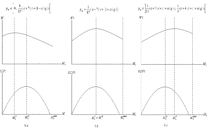
According to proposition 2, there is a level of world price for which the interests of import permit holders coincide with the objective of maximizing total welfare (condition (iii)). Figure 6 illustrates the impact of the increase in minimum access in both regions on permit holders’ rent (PHR1) and welfare (W1) of region 1, for different intervals of world price.
Figure 6.a shows that an increase in minimum access between M1* and 1
R
M decreases the total welfare of region 1. This is explained by the negative effect of increasing minimum access on the producer surplus, which outweighs the positive effect of the increase in minimum access on consumer surplus and permit holders’ rent. Beyond 1
R
M level, any increase in minimum access level lowers the producer surplus and the permit holders’ rent. Figure 6.b illustrates the case where the interests of import permit holders coincide with the objective of maximizing global welfare. In this case, an increase in minimum access beyond its optimal level decreases permit holders’ rent and the producer surplus, which outweighs the increase in consumer surplus. The final effect is a decrease in total welfare. Figure 6.c illustrates the last case, where the minimum access level maximizing the welfare of region 1 exceeds the minimum access level maximizing permit holders’ rent. In this case, the decrease in permit holders’ rent and producer surplus, between M1Rand M1*, does not exceed the increase in consumer surplus. The net effect is a rise in total welfare. Beyond M1*level, the decrease in producer surplus and permit holders’ rent is greater than the increase in consumer surplus; total welfare thus decreases in region 1.
4. Exporting from the most efficient to the least efficient region
Now, we examine the situation where the producer from region 2 acts like a monopoly on the market of its region and competes à la Cournot on the market of region 1. We therefore have
11 0
t ,t12 0, t210 and t22 0. This situation is observable if condition (2) of proposition 1 is
not met, that is: 2
13 3
w
p gc g. The solution to the problem of maximizing the producer’s profit can determine the sales solutions:
For region 1:
* 11 1 * 12 2 / 3 0 t a a g g c M t (18) For region 2:
* 21 1 * 22 2 2 / 3 / 2 t a a g c g M t a a g M (19)new conditions on sales according to minimum access level are as follows:
For region 1:
11 1 12 2 0 2 0 2 t if M a a g g c t if M a a g c g (20) For region 2: 21 1
22 2 0 2 0 ( ) t if M a a g c g t if M a a g (21)The solutions to the problem must satisfy conditions (20) and (21), which give us the conditions for which there is unilateral interregional trade from region 2 to region 1, whereas the inverse is not true. This result is explained in Corollary 2.
Corollary 2:
Exporting from the region with the lowest costs to that with the highest costs is possible
t210
, whereas the inverse is impossible
t120
only if the productive efficiency ofregion 2 relative to that of region 1 is such that
1
1
1 1 1 1 3 1 3 2 2 w 2 w Cm p Cm c < < Cm p Cm c with 2 1 Cm Cm .Figures 2.a and 2.b in Section 2 present the zone in which the region with the lowest production costs exports to the region with the highest costs, according to the transaction costs and world price respectively.
The solution of the first-order conditions of the maximization problem of the total welfare of the two regions gives us the optimal solutions of M and 1 M : 2
* 1 4 1 9 w M a a c g p (22)
* 2 3 4 w M a a g p (23)The optimal minimum access of both regions is therefore:
*
4 9 4 w 1 4 1 3
M a c p a g (24)
This will be effective for *
i w
p p (See Appendix 3). In addition, proposition 3 below shows that according to the world price and cost asymmetry, the largest region, even if it is also the most efficient, can receive a greater portion of minimum access. Low prices and/or relatively high production costs justify consumer sourcing through imports. The proof of proposition 3 is presented in Appendix 4.
Proposition 3 Let 4
5 0 3 4 w w g c g p a g p and be the size asymmetry parameter between the regions.
The largest and most efficient region is the one that:
(i) receives the smallest share of minimum access if
1 , 1
(ii) receives the same minimum access share as the other region if 1 (iii) receives the highest share of minimum access if
1 ,
. From the definition of parameter it is possible to see that the greater the cost asymmetry, the more it will be necessary, all things being equal, that the difference in size be significant for a greater minimum access level to be allocated to the large region
0
. This result is intuitive given that the large region is also the most efficient. Further, all things being equal, given that
pw 0
, the lower the world price, and the smaller the size differences, the more likely the larger region will be to receive a larger share of permits. Lastly, given that c 0, the higher the transaction costs, the more a large size difference will be necessary for the larger region to receive a larger share of import permits. All things being equal, the large region does not find it profitable to export a portion of its production toward the smaller region.5. Optimal minimum access with absence of trade between regions
In this situation there is no interregional trade, and each producer acts like a monopoly on the market of its region. We therefore have: t110,t12 0, t210 et t22 0. Then, optimal solutions must uniquely satisfy the first condition of proposition 1 on the existence of trade on each local
market, whereas the second condition of the same proposition on the presence of trade between the regions becomes:
For region 1: 12 0 2
1 3 3 w t si p gc g (25) For region 2: 21 0 1 2
3 3 w t si p g gc (26)The most constraining condition is that given by equation (26), which concerns the aptitude of the least efficient region to supply the market of the most efficient region. It is possible to
conclude that in the case where gg c and 1 2
3 3
w
g p g gc , we have
11 0
t ,t12 0, t210 and t22 0. The condition gg c implies that the lowest marginal production cost in region 2 does not suffice to compensate for the costs associated with transport costs, whereas the second condition takes global market conditions into account. This result is summarized in corollary 3.
Corollary 3
For the minimum access levels allocated to each region not to give rise to interprovincial trade, the cost asymmetry between the two regions must satisfy the following condition:
1
1 3 w 2 1 Cm p Cm c with 2 1 Cm Cm . Figures 2.a and 2.b present the zone in which there is no trade between the regions, according to transaction costs and world price respectively. Lastly, the optimal minimum access level chosen for each region is effective because *
i w
We obtain the following solutions to the problem of maximizing the producer profit in each region: For region 1:
* 11 1 * 12 / 2 0 t a a g M t (27) For region 2:
* 21 * 22 2 0 / 2 t t a a g M (28)The new conditions on sales according to the minimum access level are:
For region 1:t110 if M1a a
g
(29) For region 2:t220 if M2 a
ag
(30)The solutions of M and 1 M that maximize the total welfare of both regions issuing from the 2
first-order conditions are:
* 1 3 4 w M a a g p (31)
* 2 3 4 w M a a g p (32)and the optimal minimum access level of the set of both regions is:
*
1 4 w 1 3 1
M a a p g (33)
Equations (31) and (32) imply that when the production costs of both regions are symmetrical
under the minimum access system.18 In the case of symmetrical demand
1
, the region with the lowest marginal cost will have a smaller share of imports.196. Concluding remarks
The prevalence of import quotas in several countries and different economic sectors has generated rich literature. In Canada and the European Union, import management under tariff-rate quotas not only entails assigning eligible imports under the minimum access commitment to different provinces/countries, but also production control to guarantee a sufficiently high domestic price level. National production is allocated to different regions, each of which must mainly supply on its local market. However, the data on exchanges between provinces/countries show that in several cases, producers do not supply local markets exclusively. In Canada, this has led to conflicts between provincial administration bodies of productions under supply management, and to attempts to put in place trade barriers between provinces, which contradicts the current trend of encouraging a reduction in domestic trade barriers.20
This paper is based on the bilateral dumping model of Brander and Krugman (1983) in which trade can exist even in the absence of a comparative advantage of a given region. Reciprocal dumping is the outcome of a non-cooperative game that enhances competition while creating sourcing inefficiencies because increases in consumption are supported by purchases subject to transport costs.
18 Based on equations (31) and (32) it is possible to verify that
M
depends only on the value of and if
1 then M1*
M2*.19 Based on equations (31) and (32), we have:
3 1 0
M ag
, which implies M1* M2*.
We derive the conditions under which it is optimal to observe interregional trade and those under which trade does not exist. World price and differing production costs between regions are very influential here. In the presence of bilateral trade, the region with the largest market size will obtain the largest share of import volumes permitted under the minimum access system. When only the most efficient region exports to the least efficient region, world price, production cost asymmetry and transaction costs also play important roles in the issuing of import permits. The larger economy will not necessarily receive the largest volume of import permits. In the absence of interregional trade, the distribution of import permits between regions depends on the product cost asymmetry parameters and market size.
In terms of public policy, our results imply that even if in general countries that make minimum access commitments allocate their production between regions such that trade is strictly minimized, it is not optimal to create trade barriers between regions/countries. “Artificial” trade barriers between different regions/countries will contribute to reducing the welfare of at least one of the regions, along with global welfare. Without these barriers, world price and productivity gains observed in different regions would determine efficient adjustments to trade flows between regions/countries.
References
Baylis, K. and W. H. Furtan. 2003. Free-Riding on Federalism: Trade Protection and the.
Canadian Dairy Industry. Canadian Public Policy, 29 (2): 145-161.
Brander, J. and P. Krugman. 1983. A Reciprocal Dumping Model of International
Trade. Journal of International Economics, 15 (3-4), 313-321.
Chao, C-C, B.R. Hazari and E.S.H. Yu. 2010. Quotas, Spillovers, and Transfer Paradox
in an Economy with Tourism. Review of International Economics 18, 243-249.
Chao, C-C and E.S.H. Yu. 1991. Immiserizing Growth for a quota-distorted small
economy with variable return to scale. Canadian Journal of Economics, 24, 686-692.
Deardorff, A. V., and R. M. Stern. 1999. Measurement of Nontariff Barriers. The
University of Michigan Press, Ann Arbor, Michigan.
Feenstra, R. C., 1995. Estimating the Effects of Trade Policy. in Handbook of
International Economics, Vol. 3, ed. G. Grossman and K. Rogoff, Elsevier Science B.V.
Friberg, R. and M. Ganslandt, 2008. Reciprocal Dumping with Product Differentiation.
Review of International Economics, 16(5), 942-954.
Furtan H., J. Sauer and M.S. Jensen. 2009. Free-riding on Rent Seeking: an Empirical Analysis. Public Choice 140, 479–500.
Gervais, J-P. and H.E. Lapan, 2001. Optimal Production Tax and Quota under Time
Consistent Trade Policies. American Journal of Agricultural Economics, 83(4), 921-933.
Gervais J-P. and H.E. Lapan, 2002. Endogenous Choice of Trade Instrument Under
Uncertainty. International Economic Journal, 16(4), 75-96.
Haufler, A. and I. Wooton. 1999. Country Size and Tax Competition for Foreign Direct
Investment. Journal of Public Economics, 71(1), 121-139.
Baylis, K. and W. Hartley Furtan. 2003. Free-Riding on Federalism: Trade Protection
and the Canadian Dairy Industry. Canadian Public Policy, 29 (2): 145-161.
Kreickemeier, U. 2005. Unemployment and Well-being Effects of Trade Policy.
Canadian Journal of Economics, 39, 297-315.
Krugman, P. 1989. Industrial organization and International Trade. In Handbook of
Industrial Organization.R. Schmalensee & R. Willig (ed.). Elsevier, edition 1, volume 2, number 2.
Larue, B.; J-P. Gervais and S. Pouliot, 2008. Price equivalent tariffs and quotas under a
domestic monopoly. Journal of International Trade & Economic Development, 17(2), 311-322.
Larue, B. and R. Lambert. 2012. A Primer on the Economics of Supply Management and
Liang, W-J., H. Hwang and C-C. Mai. 2006. Spatial discrimination: Bertrand vs.
Cournot with asymmetric demands. Regional Science and Urban Economics 36, 790–802.
Maggi, G. and A. Rodrıguez-Clare. 2000. Import penetration and the politics of trade
protection. Journal of International Economics 51, 287–304
Motta, M. and G. Norman. 1996. Does Economic Integration Cause Foreign Direct
Investment? International Economic Review, 37(4), pages 757-83.
Neary, J.P. 2003. Presidential Address: Globalization and Market Structure. Journal of the
European Economic Association,1(2-3), 245-271.
Neary, J.P. 2002. Foreign Competition and Wage Inequality. Review of International
Economics 10(4), 680-93.
Neary, J. P. and J. Tharakan. 2012. International trade with endogenous mode of
competition in general equilibrium. Journal of International Economics, 86(1), 118-132.
Pouliot, S. and B. Larue. 2012. Import Sensitive Products and Perverse Tariff-Rate Quota
Liberalization, Canadian Journal of Economics, 45 (3), 903-924.
Saggi, K. and H.M. Yildiz, 2011. Bilateral Trade Agreements and the Feasibility of
Multilateral Free Trade. Review of International Economics, 19(2), 356-373.
World Trade Organization [WTO]. 2013. Trade policy review: European Union.
Available at http://www.wto.org/english/tratop_e/tpr_e/tp384_e.htm . Accessed September 04, 2013.
List of figures 30 35 40 45 50 Mi lli o n s o f d o ze n s 2002 2004 2006 2008 2010 2012 Year
Sources: Egg farmers of Canada
40 60 80 1 0 0 1 2 0 1 4 0 T h o u sa n d s o f kg 2002 2004 2006 2008 2010 2012 Year
Sources: Chicken farmers of Canada
Figure 1.a. Interprovincial trade in shell eggs Figure 1.b. Interprovincial trade in live chickens
0 .2 .4 .6 .8 1 C o st a sy mm e try p a ra me te r (a lp h a ) 0 .05 .1 .15 .2 Transaction cost (c) 0 .2 .4 .6 .8 1 C o st a sy mm e try p a ra me te r (a lp h a ) 0 .05 .1 .15 .2 World price (pw)
Figure 2.a. Effect of transaction costs and cost
asymmetry parameter on regions’ capacity to trade with each other
Figure 2.b. Effect of world price and cost
asymmetry parameter on regions’ capacity to trade with each other
12 21 0 t t 12 0; 21 0 t t 12 0; 21 0 t t 12 21 0 t t 12 0; 21 0 t t 12 0 ; 21 0 t t
Figure 3. Impact of minimum access on welfare of the two regions
Figure 5. Impact of minimum access on consumer surplus in region 1
Appendices
Appendix 1.Proof of proposition 1
According to this case, there is no corner solution: all sales are observed. Optimal quota solutions must satisfy the conditions of (17), which let us obtain the following conditions:
For region 1:
11 2 1 0 3 3 t if pw g gc (34)
12 2 1 0 3 3 t if pw gc g (35) For region 2:
21 1 2 0 3 3 t if pw g gc (36)
22 1 2 0 3 3 t if pw g c g (37)Condition (35) is the most restrictive. If it is satisfied then t110, t12 0, t210 and t22 0. If the optimal quota chosen for each region M , for alli* i1, 2 , is defined by (15) and it is
effective for *
i
p pw. Further, the solution of the model gives identical prices in both regions,
namely: *
3 1
i
p pw gc. Condition:p*i pw, which implies 1 1
2 2
pw g gc
because condition 2
13 3
pw gc g is the most restrictive.
Appendix 2. Proof of proposition 2
Import permit holders in region 1 maximize their rent:
1 * 1 1 max w M p p M
1 1 1 3 max 3 M a a c g pw g M M a The maximum rent for a value of imports to region 1 that verifies the following equation:
1 1 3 2 : 0 3 a a c g pw g M M a This gives the solution:
1 1 1 3 2 R M a a c g pw We therefore have:
1 0 / 3 R M if pw a c g g (38) The minimum access level that maximizes total welfare is:
* 1 1 4 1 9 w M a a c g p
* 1 0 4 1 / 9 M if pw a c g (39) Condition (39) is more restrictive than condition (38):
1
9 4 1 3 2 w p c g pw c g g pw ggc (40) Condition (40) is less restrictive than condition 1
2 2
3
w
p gg c , which is defined in
proposition 1: 1
1
2 2
2 ggc 3 gg c g g c.
Let us now calculate the difference, *
1 1 R M M :
* 1 1 1 7 7 15 7 2 R R a M M M a c g pw g We can conclude that:
1 1 1 1 0 0, 7 1 15 1 1 0 7 1 , 4 1 15 9 1 0 7 1 15 R w R w R w M if p a c g M if p a c g a c g M if p a c g Appendix 3. Condition of efficiency of optimal minimum access when the most efficient region exports to the least efficient region
The price in region 1 is: p1*3pw
1
gc *1 w
p p which implies that
1 1
2g2 g c pw. This condition is satisfied for gg c because
1 2g1 2 g c 2 3g 1 3 gc and in the case where gg c because
1 2g1 2 gc 1 3g2 3 gc . Therefore, we can conclude that the minimum access level of region 1 is effective regardless of g
gc. In region 2, the equilibrium price is*
2 2 w
p p g p2* pw which implies that g pw. This condition is satisfied when
gg c because g2 3g1 3
gc
and in the case where gg c because
1 3 2 3
g g g c
. It is therefore possible to conclude that the minimum access level of region 2 is effective regardless of g
gc.Appendix 4. Proof of proposition 3
Let us define by M the difference between the optimal minimum access level for region 1 and that of region 2:
* * 1 2 1 4 4 9 w 4 1 3 M M M a a c p g (41)Based on (41), it is possible to show that * *
1 2
M M only when 1 with
4 5 0 3 4 w w g c g p a g p . Accordingly, 4
g c
g5pw0 and a3g4pw 0because 4
g c
g5pw 0, which implies that pw4 5
g c
1 5g. However, thecondition pw 2 3
g c
1 3g is more restrictive: 2 3
g c
1 3g4 5
g c
1 5gwhich implies that g c g. The optimal access level in region 2, M2*, must be strictly positive: M2* 0, which implies that a3g4pw 0.
Appendix 5. Condition of efficiency of optimal minimum access when there is no trade between regions
The price in region 1 is *
1 2 w
p p g and we have p1* pw, which implies that g pw becausegpw1 3g2 3
gc
. In region 2, the equilibrium price is *2 2 w
p p g and *
2 w