Fagart: Université Paris Descartes
Fluet: Corresponding author: Université du Québec à Montréal and CIRPÉE
Cahier de recherche/Working Paper 14-05
Risk Aversion and Incentives
Marie-Cécile Fagart Claude Fluet
Abstract:
We consider decision-makers facing a risky wealth prospect. The probability distribution depends on pecuniary effort, e.g., the amount invested in a venture or prevention expenditures to protect against accidental losses. We provide necessary local conditions and sufficient global conditions for greater risk aversion to induce more (or less) investment or to have no effect. We apply our results to incentives in the principal-agent framework when differently risk averse agents face the same monetary incentives.
Keywords: Expected utility, risk aversion, comparative statics, mean utility preserving
increase in risk, location independent risk
1
Introduction
We consider decision-makers facing a risky wealth prospect. The probabil-ity distribution depends on pecuniary e¤ort, e.g., the amount invested in a venture or prevention expenditures to protect against accidental losses. The issue is the relation between risk aversion and the decision-maker’s e¤ort. This line of inquiry has a long history.1 We review the literature most rel-evant for our paper at the end of the introduction. Our contribution is to characterize the necessary “local”or “…rst-order”conditions for greater risk aversion to induce more (or less) e¤ort and to provide “global” conditions ensuring that the necessary conditions are also su¢ cient.
To illustrate our approach, consider the so-called LEN model (for l inear exponential normal, see Holmstrom and Milgrom 1987). A decision-maker can invest the amount a in a project yielding a normally distributed gross return Y . The variance is constant and the mean is the concave function (a). The net return is W Y a. As is well known, all decision-makers with CARA utility functions invest the same amount as would a risk neutral, i.e., they choose aN maximizing the expected …nal wealth. When the solution is interior, it satis…es the …rst-order condition 0(a
N) = 1. However, the same is also trivially true of all risk averse individuals. Indeed, denoting the utility function by u( ), the marginal expected utility with respect to a can be written as
( 0(a) 1)E[u0(W )j a]:
Normally distributed gross returns with a constant variance is thus one ex-ample of situations in which risk aversion has no e¤ect on e¤ort. The result is trivial because the …nal wealth distributions at di¤erent investment levels
1See for instance the insurance and economics of risk literature, notably Ehrlich
and Becker (1972), Dionne and Eeckhoudt (1985), Boyer and Dionne (1989), Briys and Schlesinger (1990), Jullien and al. (1999). More recently Chiu (2005), Eeckhoudt and Gol-lier (2005), and Meyer and Meyer (2011) discussed the role of prudence in self-protection decisions.
can be ranked on the basis of …rst-order stochastic dominance.
a
)
(a
σ
1a
Na
a
a
)
−
(
µ
a
)
(a
σ
1a
Na
a
a
)
−
(
µ
a
)
(a
σ
1a
Na
a
a
)
−
(
µ
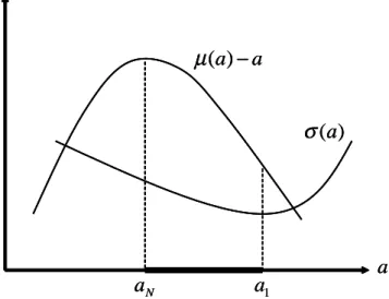
Figure 1. Normally distributed returns
But suppose that the amount invested also a¤ects the standard deviation (a). The marginal expected utility is now2
( 0(a) 1)E[u0(W )j a] + 0(a) (a)E[u00(W )j a]:
Obviously, risk neutral decision-makers continue to choose aN. This is not so for risk averse individuals. For instance, when 0(a
N) < 0, the expected utility of a risk averse is strictly increasing in a at aN. Risk averse decision-makers would therefore be expected to invest more. This must be so when the situation is as represented in Figure 1. With normally distributed returns, the …nal wealth distribution at aN second-order stochastically dominates the distributions at all a below aN. All risk averse decision-makers therefore pre-fer aN to any a < aN. Similarly, noting that the variance is minimized at a1,
2The expected utility is Ru( a + z) (z) dz where (z) is the standard normal
density. The marginal expected utility is then Ru0( )[ 0 1 + 0z] (z) dz. Noting that
z (z) = 0(z) and integrating by parts, Z
u0( )z (z) dz = E[u00
j a], which yields the second term.
the distribution at a1 second-order stochastically dominates the distributions at a > a1. Thus, all risk averse decision-makers will choose an action in the open interval (aN; a1). The set of second-degree undominated actions is the thick interval in the …gure.
One can go a step further. Suppose someba is optimal for a particular risk averse. Because 0(ba) < 0, one can show that the expected utility of a more risk averse is then increasing at ba (and decreasing for a less risk averse). A more risk averse will then invest more than ba. The result follows because, with (a) concave and (a) convex as represented in Figure 1, expected utility can be shown to be concave in the amount invested.3 Altogether, we therefore have a situation where, given the actionba chosen by some decision-maker, the choices of more or less averse decision-makers can be predicted solely on the basis of the sign of 0(ba), i.e., depending on whether risk is “locally” increasing or decreasing with the amount invested.
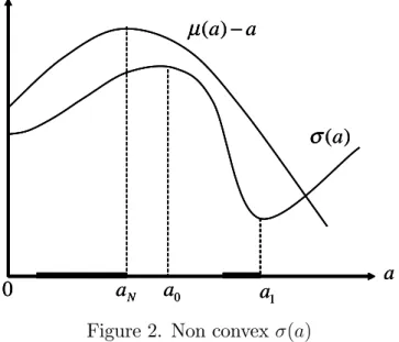
Suppose, however, that the situation is as represented in Figure 2. Now (a) reaches a maximum at a0 > aN and a minimum at a1 > a0. A risk neutral continues to choose aN. Because 0(aN) > 0, a slightly risk averse will choose to invest an amount slightly below aN. A somewhat more risk averse than the latter individual would invest an even smaller amount. However, a very risk averse decision-maker will invest more than aN, e.g., he will prefer an action just slightly below a1. The expected …nal wealth is then signi…cantly smaller but the risk is su¢ ciently reduced to make this worthwhile for a very risk averse. In the situation described by Figure 2, expected utility will generally not be concave in a. Indeed, the set of second-degree undominated actions is the union of the two disjoint thick intervals represented in the …gure.4 The example illustrates the following related points. First, when
3Di¤erentiate expected utility once more with respect to a and use the same argument
as in footnote 2. See section 4 for a more general proof in the case where variables are not normally distributed.
expected utility cannot be guaranteed to be concave or quasiconcave, the direction of local changes in risk will not allow any …rm prediction about the actions chosen by more (or less) risk averse decision decision-makers. Secondly, there are then no general conditions ensuring a monotonic relation between action and risk aversion.
a
)
(a
σ
1a
Na
a
a
)
−
(
µ
0a
0
a
)
(a
σ
1a
Na
a
a
)
−
(
µ
0a
0
a
)
(a
σ
1a
Na
a
a
)
−
(
µ
0a
0
Figure 2. Non convex (a)
This paper provides necessary and su¢ cient conditions for generalizing to arbitrary distributions the kind of results illustrated in Figure 1. Suppose ba is the optimal action of some decision-maker. We …rst ask whether di¤er-ently risk averse decision-makers would gain by marginally deviating fromba? This yields “local” or “…rst-order” conditions on the distribution of returns for risk aversion to be either locally incentive-neutral, incentive-increasing or decreasing. Next we look at the global maxima of individuals with a utility function di¤ering from that of the reference individual. We show that our “local” conditions for characterizing the relation between risk aversion and action are necessary for the same relation to hold with respect to global max-ima. Speci…cally, for all more risk averse to invest more than ba, it must be variance.
the case that expected utility is increasing in a at ba for all more risk averse. It follows that, if expected utility is concave in a, the “local”necessary con-ditions are also su¢ cient for all more risk averse to invest more. We provide conditions for the decision-makers’ problem to be concave. The conditions are shown that to bear no particular relation with how risk varies around ba. Hence the concavity condition can be combined with “local” conditions ensuring that greater risk aversion is either incentive increasing or decreasing. In a seminal paper, Diamond and Stiglitz (1974) introduced the notion of mean utility preserving increase (or decrease) in risk. They use the concept to analyze the e¤ect of risk aversion on behavior in various contexts. Applied to a problem such as ours, their analysis is purely in terms of local comparative statics results: given the action chosen by some reference decision-maker, a marginally more risk averse individual gains by investing marginally more (or less). This sides step the di¢ culties raised in the example illustrated in Figure 2. By contrast, we obtain the same condition as Diamond and Stiglitz’ as a necessary condition for all more risk averse to invest more. Next we provide conditions ensuring that the local characterization of changes in risk is su¢ cient to predict global optima. An important feature, as mentioned above, is that the global conditions have no bearing on local changes in risk. The analogy with the example of Figure 1 is that the conditions 00 0 and
00 0 imply nothing concerning the sign of 0(ba).
Another important contribution is Jewitt’s (1989) notion of location inde-pendent risk. The notion is important because it can be used to characterize the “dispersion”of gross returns independently of the amount invested (or of the individual’s initial wealth). Applied to our problem, one can show that a su¢ cient condition for a monotonic relation between risk aversion and ac-tion is that locaac-tion independent risk be monotonic in the amount invested. However, the assumption of overall monotonicity would not …t the example illustrated by Figure 1 where risk is …rst decreasing then increasing. Both the notions of mean utility preserving increase in risk and location independent
risk nevertheless play an important role in our analysis as a characterization of local changes in risk.
Section 2 sets out the decision problem and reviews notions of risk and dispersion. Section 3 derives the necessary condition. Section 4 compares global optima and presents examples. Section 5 applies the results to incen-tives in the principal-agent model when e¤ort has a money cost. Section 6 concludes. All proofs are in the Appendix.
2
Set-up
Individuals invest a 2 [0; a] in a prospect yielding the gross return y, so that …nal wealth is w = y a. Returns are realized according to the distribution G(y j a), where G is twice-continuously di¤erentiable with density denoted by g. For all a, the support is contained in Y [y; y], where the bounds need not be …nite. Utility functions are strictly increasing in …nal wealth, concave, and twice-continuously di¤erentiable. We denote by U the set of all such utility functions de…ned over [w; w] [y a; y].
Individuals will be referred to by their utility function in U. We write utility functions as lower-case letters and use the corresponding upper case for the expected utility. For decision-maker u, the expected utility from investing a is
U (a) Z y
y
u (y a) g(y j a) dy: (1)
We consider distributions of returns such that (1) exists.
Our purpose is to compare the choices of decision-makers who di¤er in risk aversion, including risk neutrality as a limiting case. Individual v is more risk averse than individual u if v is a nondecreasing concave transformation of u or equivalently
v00(w) v0(w)
u00(w)
Note that di¤erences in risk aversion may be due to di¤erences in wealth, e.g., one could write u(y a) (wu
0 + y a) where w0u is individual u’s initial wealth.
Various notions of risk and stochastic orders will prove useful. Diamond and Stiglitz’ (1974) mean utility preserving increase in risk, hereafter DS-riskiness, is de…ned with respect to a reference individual. Denote the dis-tribution of …nal wealth by H(w j a), so that H(w j a) G(w + a j a). Distributions can be thought of as being indexed by a. By de…nition, a2 is DS-riskier than a1 with respect to the utility u if individual u is indi¤erent between a1 and a2 while all individuals more risk averse than u prefer a1. This property is equivalent to
w Z w u0( )H( j a1) d w Z w u0( )H( j a2) d for all w; (3) w Z w u0( )H( j a1) d = w Z w u0( )H( j a2) d : (4)
When the reference individual is risk neutral so that u0 is constant, (3) and (4) imply that a2 is a mean preserving spread of a1. With u0 constant, condition (3) on its own means that a1 second-degree stochastically dominates a2. All risk averse individuals then prefer a1 (at least weakly) and so does a risk neutral.
Jewitt’(1989) location independent risk, hereafter J-dispersion, does not rely on a reference individual. It ranks distributions independently of hor-izontal shifts in the distributions.5 The notion generalizes the idea that a normally distributed variable is more risky than another if it has a larger variance, irrespective of the means. J-dispersion can therefore be applied di-rectly to gross returns. The distribution of returns a2 has more J-dispersion
5On these notions, see also Landsberger and Meilijson (1994) and Chateauneuf et al.
than a1 if Q(p;aZ 1) y G(yj a1) dy Q(p;aZ 2) y
G(yj a2) dy for all p 2 (0; 1), (5)
where Q(p; a) denotes the quantile function associated with G(y j a), i.e., Q(p; a) is the p-percentile gross return. Because our cumulative distributions are strictly increasing in y, the quantile is simply the inverse function de…ned by
G(Q(p; a)j a) p for all p 2 (0; 1): (6) Using the change of variable y = Q(p; a) and integrating by parts, condition (5) can be rewritten as p Z 0 Qp( ; a1) d p Z 0 Qp( ; a2) d for all p 2 (0; 1): (7)
We will also sometimes refer to the following stronger condition. The distribution of returns a2 is more dispersed than a1 in the sense of Bickel and Lehmann (1979), hereafter BL-dispersion, when Q(p; a2) Q(p; a1) is non decreasing in p, i.e., when
Qp(p; a1) Qp(p; a2)for all p 2 (0; 1): (8) Obviously, (8) implies 7.
Finally, it will also be useful to express the condition of second-degree stochastic dominance in terms of quantiles (see Levy 1992). The quantile function of …nal wealth is Q(p; a) a. The distribution a1 second-degree dominates a2 if p Z 0 (Q( ; a1) a1) d p Z 0 (Q( ; a2) a2) d for all p 2 (0; 1): (9)
3
Necessary conditions
Decision-makers choose a to maximize expected utility. An interior maximum for individual u satis…es the …rst-order condition
U0(a) = Z y
y
u0(y a) (Ga(y j a) + g(y j a)) dy = 0: (10) We assume throughout that maxima are interior. We …rst analyze necessary conditions for all more risk averse individuals to invest more (or less) than some reference decision-maker.
Local incentives. The necessary conditions are in terms of “local in-centives”, by which me mean what happens in the neighborhood of some action.
De…nition 1 Let U0(a
u) = 0 for decision-maker u. Risk aversion is (i) incentive-neutral at au if V0(au) = 0 for all v; (ii) incentive-increasing (resp. decreasing) at au if V0(au) 0 (resp. 0) for all v more risk averse than u, with strict inequalities for some v.
Incentive-neutrality means that, if au is a stationary point for individual u, then the same is true for all decision-makers irrespective of their degree of risk aversion. Risk aversion is incentive-increasing when all more risk averse decision-makers weakly prefer to marginally increase their investment above au and some strictly so.
Proposition 1 Let U0(au) = 0 for decision-maker u. Risk aversion is (i) incentive-neutral at au if and only if
Ga(y j au) + g(yj au) = 0, for all y2 Y; (11) (ii) incentive-increasing at au if and only if, with strict inequalities over some interval,
Z y y
and is incentive-decreasing when the reversed inequalities hold.
When au is in fact optimal for individual u, condition (11) is necessary for all individuals to also want to choose au. It turns out that the local condition (12) is itself necessary for the optimal choice of all more risk averse individuals to be above au.
Proposition 2 Let au and av be optimal for the individuals u and v respec-tively. If av = au for all v, then (11) holds. If av au for all v more risk averse than u, then (12) holds; if av au for all v more risk averse than u, the reverse inequalities hold.
The second part of the proposition rules out the possibility that a decision-maker would prefer to marginally decrease his investment below au while his global maximum is in fact above au. Slightly di¤erent individuals can be expected to make only slightly di¤erent choices, i.e., there will be some whose best action is arbitrarily close to au. For all decision-makers more risk averse than u to invest more than au therefore requires the expected utilities of slightly di¤erent decision-makers to be non-decreasing at au. The proposition shows that the same must in fact be true for all more risk averse decision-makers.6
Local changes in risk and dispersion. We now interpret our necessary conditions in terms of risk and dispersion. Proposition 2 imposes conditions on the distribution of …nal wealth, which we denoted H(w j a). Consider …rst the case where all individuals in U optimally choose au. It must then be
6We focused on more risk averse decision-makers when (12) or the reverse inequalities
hold. Because the condition is necessary and su¢ cient for risk aversion to be locally in-creasing (or dein-creasing), the implications for less risk averse decision-makers are perfectly symmetrical.
that au second-degree stochastically dominates all a. This requires w Z w H( j au) d w Z w
H( j a) d for all w and a.
The expression on the right-hand side is therefore minimized at au, for all w. Because the minimum is interior, the necessary …rst-order condition is
w Z
w
Ha( j a) d = 0 for all w.
Di¤erentiating with respect to w then yields Ha(w j au) = 0 for all w. Condition (11) follows by noting that
Ha(y aj a) Ga(y j a) + g(y j a):
Thus, (11) is the …rst-order condition for second-degree stochastic dominance at au.
It may be remarked that (11) is also the order condition for …rst-degree stochastic dominance at au. The requirement is then H(w j au) H(w j a) for all a and w, which again implies Ha(w j au) = 0 for all w. Obviously, if there exists a …rst-degree dominant action, it will also be second-degree dominant. In the case of normally distributed returns represented in Figure 1, aN is second-degree dominant when (a) also reaches its minimum at aN (i.e., when a1 = aN). However, unless (a) is constant, there is then no …rst-degree dominant action.
Consider now condition (12) when au is optimal for u. In terms of the distribution of …nal wealth at au and au+", where " is positive but negligible,
w Z w u0( ) (H( j au+ ") H( j au)) d ' " w Z 1 u0( )Ha( j au) d :
Because decision-maker u’s expected utility is maximized at au, a small change has only second-order e¤ects, i.e., the right-hand side vanishes at
w = w. Given condition (12), however, the right-hand side is non positive for all w w when " > 0. The condition therefore states that a marginally larger investment level is DS-less risky than au with respect to u. Hence, it is preferred by decision-makers more risk averse than u.
We now turn to the notions of dispersion introduced in section 2. These can be de…ned in the neighborhood of a given action, noting that for " arbi-trarily small Qp(p; a + ") Qp(p; a)' "Qap(p; a):
De…nition 2 BL-dispersion is locally decreasing in a if Qap(p; a) 0 for all p. J-dispersion is locally decreasing in a if R0p Qap( ; a) d 0 for all p. Dispersion is stationary if the equalities hold for all p.
From (6), it is easily seen that Qp(p; a) = g(Q(p; a)j a) 1 and Qa(p; a) =
Ga(Q(p; a) j a)
g(Q(p; a)j a) for p 2 (0; 1):
Condition (11) is therefore equivalent to Qa(p; au) = 1 for all p. It follows that Qap(p; au) = 0 for all p, i.e., condition (11) implies that dispersion is stationary at au.
BL-dispersion decreasing at au implies (12). To see this, write expected utility in terms of the quantile function,
U (a) = Z 1
0
u(Q(p; a) a) dp: (13)
Expected utility is stationary at au when U0(au) =
Z 1 0
u0(y au) (Qa(p; au) 1) dp = 0: (14) Similarly, (12) can be rewritten as
Z p 0
u0(y au) (Qa( ; au) 1) d 0 for p 2 (0; 1): (15) Given condition (14), Qa(p; au) 1cannot be always positive or always neg-ative. When Qap(p; au) 0 for all p, the expression is nonincreasing in p
and must therefore change from positive to negative. Hence, BL-dispersion decreasing at au implies (15). We show that J-dispersion decreasing at au also implies (15).
Corollary 1 Given U0(a
u) = 0, condition (11) is equivalent to dispersion being stationary at au; J-dispersion decreasing at au implies condition (12):
Discussion. When u optimally chooses au, condition (12) is necessary for all individuals more risk averse than u to invest more than au. However, the condition is not su¢ cient by itself to predict global optima, unless expected utility can be guaranteed to be concave or pseudoconcave in the amount invested.7 The next section will provide su¢ cient conditions.
Even when one abstracts from these issues, it should be emphasized that a condition such as (12) does not yield an overall monotonic relation between optimal actions and risk aversion. Speci…cally, it may well be that some other individual v, who cannot be ranked in terms of risk aversion with respect to u, also optimally chooses au. For individual v, the equivalent of condition (12) may not hold, even though it holds for u. Hence, because the condition is necessary to allow predictions, there will be some individuals more risk averse than v who will invest less than v and some who will invest more.
We brie‡y discuss the implications of overall monotonicity between action and risk aversion. Let A fa j a 2 arg maxa0U (a0), u 2 Ug. When A is
not a singleton, it is the set of actions which cannot be ranked by second-degree stochastic dominance. In other words, any action in this set is some individual’s optimal choice. An example is the interval [aN; a1) in Figure 1 for the case of normally distributed returns.
Corollary 2 Let au and av denote the optimal actions for u and v respec-tively. If A is convex and av au for all u, v 2 U with v more risk averse
7A continuously di¤erentiable quasiconcave function is pseudoconcave if a vanishing
than u (alternatively av au), then U (a) is quasiconcave over A for all u2 U.
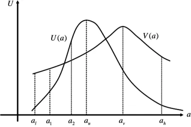
Figure 4 provides an illustration. The set A is the interval from al to ah. According to the corollary, each decision-makers’ expected utility is single-peaked over the set of relevant actions. This follows from Proposition 2. In the …gure, v is more risk averse than u and av > au. Hence, v’s expected utility is non-decreasing at au. But the same is also true for all a < av because any such a is chosen by some less risk averse than v. A similar argument shows that v’s expected utility is everywhere non-increasing to the right of av (see the Appendix for the details).
Overall monotonicity requires strong conditions on G. In the next section, we do not impose such strong conditions. Our focus is the use of the local conditions of Proposition 1 for predicting behavior.
a u a U ) (a U 1 a av ah l a a2 ) (a V a u a U ) (a U 1 a av ah l a a2 ) (a V
Figure 3. Monotonicity and quasiconcavity
4
Local incentives as su¢ cient conditions
Given the action optimally chosen by individual u, the conditions of Proposi-tion 1 are su¢ cient for predicting the choices of more (or less) aversedecision-makers if expected utility is concave in e¤ort for all decision-decision-makers. Recall-ing the quantile expression for expected utility in (13), a straightforward su¢ cient condition is the concavity in a of the quantile function Q(p; a), equivalently G(y j a) quasiconvex in y and a. A weaker condition is Concav-ity of the Cumulative Quantile (CCQ) as de…ned in Fagart and Fluet (2013). They show that the condition is su¢ cient for expected utility to be concave in a for all risk averse (or risk neutral) decision-makers.
De…nition 3 The distribution G(y j a) satis…es CCQ if R0pQ( ; a) d is con-cave in a for all p, equivalently if RyyG( j a) d is convex in (y; a).
When the gross return distribution satis…es CCQ, condition (11) implies that all decision-makers also choose au; condition (12) implies that all more risk averse decision-makers invest more than au. We discuss two examples illustrating how quantile concavity or the weaker CCQ combine with local changes in dispersion.
Multiplicative-additive risk model. Let the gross return be a linear function of some random state, i.e., y = (a) + (a)z where (a) > 0 and z is the realization of the random variable Z which does not depend on a. This generalizes the case of normally distributed returns discussed in the introduction. Without loss of generality, we can take Z to have zero mean and unit variance, hence (a) and (a) are respectively the mean and the standard deviation of returns.
Let QZ(p) denote the quantile function of Z. The zero mean condition is R1
0 QZ(p) dp = 0. The gross return quantile is
Q(p; a) = (a) + (a)QZ(p):
We assume 00(a) 0 and 00(a) 0. These conditions guarantee that the distribution of returns satisfy CCQ: for all p,
Z p 0 Qaa( ; a) d = p 00(a) + 00(a) Z p 0 QZ( ) d 0:
The integral on the right-hand side is negative because it has the same sign as the mean of the distribution truncated from the right.
Let au be individual u’s optimal action. Recalling the quantile formula-tion of second-degree stochastic dominance in (9), observe that
Z p 0 (Qa( ; au) 1) d = p ( 0(au) 1) + 0(au) Z p 0 QZ( ) d
cannot be positive (or negative) for all p. If it were, a marginal variation from au would second-degree dominate, contradicting the statement that au is optimal.
There are therefore three possibilities. The …rst is 0(a
u) 1 = 0(au) = 0, implying that expected …nal wealth is maximized and that its variance is minimized. Noting that Qap(p; a) = 0(a)Q0Z(p), this possibility corresponds to the case where condition (11) holds and dispersion is stationary at au. The action au is then second-degree dominant and all decision-makers also choose au.
The two other possibilities are either 0(a
u) > 1together with 0(au) > 0 or 0(a
u) < 1 together with 0(au) < 0. When 0(au) < 0, BL-dispersion is decreasing at au. Individual u invests more than the amount that would max-imize expected wealth because this allows him to “purchase”less dispersion. Condition (12) then holds, implying that more risk averse decision-makers will invest even more than u. When 0(au) > 0, BL-dispersion is increasing at au. Individual u invests less than the the amount maximizing expected wealth because this would come at the cost of too much dispersion. More risk averse individuals will then invest even less.
Stochastic production function. Consider now a general stochastic production function with a as input, y = '(a; z) where 'a > 0, 'aa < 0 and 'z > 0, i.e., large values of z correspond to more favorable states of Nature. The gross return quantile is then Q(p; a) = '(a; QZ(p)). Concavity in a follows from the concavity of the production function, hence expected utility is concave in a. Note that Qap(p; a) = 'az(a; QZ(p))Q0Z(p).
Suppose decision-maker u optimally chooses au. If 'az(au; z) < 0 in all states of Nature, BL-dispersion is decreasing at au. Individuals more risk averse than u invest more because the marginal product of investment is relatively larger in unfavorable states of Nature.8 More risk averse individuals are more willing than u to trade o¤ a smaller net wealth in favorable states against a larger net wealth in unfavorable ones. Conversely, if 'az(au; z) > 0 in all states, BL-dispersion is increasing at au and more risk averse individuals invest less than u.
A more general case is to allow 'az(au; z)to change sign. For instance, it may be that the marginal product 'a is below average when Nature is either very harsh or very generous; conversely that it is above average in extreme conditions, whether favorable or unfavorable. J-dispersion is decreasing at
au if Z p
0
'az(au; QZ( ))Q0Z( ) d 0 for all p: Integrating by parts, this can be rewritten as
'a(au; QZ(p)) 1 p Z p 0 'a(au; QZ( )) d for all p: (16) The expression on the right-hand side is the average marginal product below the p-percentile. Condition (16) is equivalent to
d dp 1 p Z p 0 'a(au; QZ( )) d 0 for all p:
In words, J-dispersion is decreasing at au when the marginal product is on average larger in unfavorable states. Individuals more risk averse than u then invest more.
First versus second-degree stochastic dominance. When disper-sion is stationary at some given action and the distribution of returns satis…es
8This is essentially the case discussed in Jullien et al. (1999). Their Propositions 5 and
6 are both equivalent to the condition that BL-dispersion is decreasing at all a. Observe that 'az(au; z) < 0 for all z only means that BL-dispersion is locally decreasing at au.
CQC, all risk averse or risk neutral decision-makers optimally choose that action. In other words, the local condition (11) is then both necessary and su¢ cient for the action to be second-degree dominant. In some cases the action may also be …rst-degree dominant and will be so if a …rst-degree dom-inant action exists.
In section 3, we remarked that the same condition (11) was also necessary for …rst-degree stochastic dominance at the action considered. Are there con-ditions that would allow us to infer …rst-degree stochastic dominance when (11) holds? For this purpose, we consider an alternative characterization of decreasing returns to investment. The condition will be referred to Isoprob-ability Convexity of the Distribution Function (ICDF).
De…nition 4 The distribution of returns satis…es ICDF if Ga(Q(p; a)j a) is nondecreasing in a for all p and a.
The condition evokes the well known Convexity of the Distribution Func-tion CondiFunc-tion (CDFC) de…ned by Ga(y j a) nondecreasing in a for all y. However, ICDF looks at convexity for given probability levels. When a larger a increases returns in the sense of …rst degree stochastic dominance, Ga(y j a) is the marginal productivity in terms of reducing the proba-bility of outcomes worse than y. Similarly, Ga(Q(p; a) j a) is the p-level marginal productivity. ICDF imposes that p-levels marginal returns be de-creasing. The condition is easily shown to be equivalent to Ga(y j a)=g(y j a) nondecreasing in a.
Corollary 3 Suppose U0(a
u) = 0 and dispersion is stationary at au. If the distribution of returns satis…es CCQ, au is second-degree stochastically dom-inant. If it satis…es ICDF, au is …rst-degree dominant.
When dispersion is stationary at au, ICDF ensures that the net return quantile, Q(p; a) a, is nondecreasing in a for a < au and nonincreasing otherwise; that is, the net return quantile is quasiconcave and reaches a
maximum at au for all p. Hence au is …rst-degree dominant.9 There is some overlap between CCQ and ICDF. For instance, Ga always nonpositive, ICDF and BL-dispersion everywhere nonincreasing can be shown to imply CCQ.10
5
An application to incentive schemes
We apply the preceding results to incentives in the principal-agent frame-work with moral hazard. E¤ort is pecuniary, i.e., an unveri…able monetary expenditure. The principal faces many di¤erent agents and is constrained to use the same performance scheme with all of them. The issue is how agents with di¤erent risk preferences react to the same monetary incentives.
The wage or payment depends on the signal X, e.g., the agent’s output or a purely informative performance index. The cdf is denoted (xj a), the corresponding density is (x j a) with a support X [x; x]that is invariant with respect to e¤ort. We make the usual assumptions that is twice continuously di¤erentiable and satis…es MLRP with a= strictly increasing in x so that a < 0. Given an increasing wage scheme, the marginal gross return of e¤ort is positive in the sense of …rst degree stochastic dominance.
We show that the e¤ect of risk aversion depends on the curvature of the payment scheme, where curvature is in terms of an appropriate transforma-tion of the signal. Loosely speaking, when the wage scheme is “concave”, risk aversion will be incentive increasing; it will be incentive decreasing when the scheme is “convex”.
For some e¤ort levelba, consider the transformed signal Z de…ned by z = '(x) x Z xc ( j ba) a( j ba) d , x 2 X; (17)
9The reverse condition, G
a(Q(p; a) j a) nonincreasing in e¤ort, would imply that the
expected utility reaches a global minimum when dispersion is stationary at au. 10MLRP (i.e., g
a=g increasing in y), ICDF and Jewitt-dispersion everywhere decreasing
where xc is some arbitrary threshold of the original signal. Denote the sup-port of the transformed signal by Z [z; z]. Because ' is a strictly increasing function, Z also satis…es MLRP and delivers the same information as X with respect to a. Hence, any wage scheme de…ned with respect to the original signal can be replicated as a scheme de…ned with respect to the transformed signal. We henceforth focus on the latter and represent a wage scheme by a function y = y(z).
As a …rst observation, under a scheme of the form y(z) = z, risk aversion is incentive-neutral atba. To see this, observe that the resulting random wage is distributed according to the cdf F (z j a) = (' 1(z)
j a) with density f (z j a) = (' 1(z)
j a)d' 1(z)=dz. Noting that d' 1(z)
dz =
a(' 1(z)j ba) (' 1(z)j ba) ;
it follows that Fa(z j ba) + f(z j ba) = 0 for all z, i.e., condition (11) of Proposition 1 holds at ba. The same would be true of any linear scheme y(z) = z + k where k is an arbitrary constant. We now look at the e¤ects of non linearity.
Corollary 4 Under the wage scheme y(z), BL-dispersion is decreasing at ba if and only if y00(z) 0 for all z. J-dispersion is decreasing at ba if and only if E[y0(Z)j Z z;ba] is decreasing in z for all z:
Decreasing BL-dispersion at ba is equivalent to the concavity of the pay-ment scheme compared to the linear benchmark. Under concave schemes, a marginal increase in e¤ort above ba reduces the riskiness of the wage dis-tribution; the opposite occurs with convex schemes. The interpretation with respect to J-dispersion is similar. J-dispersion is decreasing at ba when the scheme is “concave on average”, i.e., the slope of the wage function is on average larger at the bottom the distribution. The intuition is that whether risk aversion is incentive increasing or decreasing depends on the location of incentives with respect to realizations of the signal.
We now provide a characterization in terms of condition (12) of Proposi-tion 1.
Corollary 5 Suppose U0(ba) = 0 under the scheme y(z) and de…ne f u(z) u0(y(z) ba)f(z j ba). Then
Z z z
(y0(z) 1)fu(z) dz = 0 (18)
and risk aversion is incentive increasing at ba if and only if z
Z z
(y0( ) 1)fu( ) d 0 for all z. (19)
The function fu(z) can be interpreted as a density because utility func-tions are arbitrary up to an increasing linear transformation. Condition (19) describes a scheme tilted towards penalizing the agent for bad performance rather than rewarding him for good performance.
When u is risk neutral, fu(z) f (z j ba). The conditions (18) and (19) then reduce to
E[y0(Z)j ba] = 1; (20)
E[y0(Z)j Z z;ba] 1 for all z: (21) A risk neutral agent is motivated only by the overall expectation of the slope. He is indi¤erent to whether the slope is on average greater at the bottom or at the top of the distribution. This is not so for a risk averse agent. Given (21), the expected utility of a risk averse is increasing at ba: exerting more e¤ort yields a mean preserving contraction in the agent’s random wage. The opposite obtains when the inequalities are reversed. When agent u is himself risk averse, condition (19) together with (18) imply that the density fu puts greater weight on bad outcomes compared to good ones. A more risk averse agent would put even greater weight on bad outcomes.
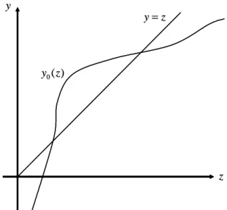
z ) ( 0 z y y z y= z ) ( 0 z y y z y=
Figure 4. A penalty oriented scheme
Figure 4 provides an illustration. In the …gure, y0(z) 1is …rst positive then negative as z increases. The single-crossing property implies that, if (20) holds, then (21) must also hold. Similarly, if (18) holds, then so must (19).
Because a risk averse agent is sensitive to the location of the incentives, it is possible to induce e¤ort with a scheme that is not very steep overall, provided it has su¢ cient “power” in the lower tail. The more risk averse the agent, the more the slope in the lower tail will matter compared to that in the upper tail. Therefore, depending on the location of incentives, wages that provide risk neutral agents with relatively weak incentives may provide strong incentives for risk averse ones. Conversely, a reward-oriented scheme that provides good incentives for a risk neutral may work poorly with risk averse individuals.
6
Concluding Remarks
We derived necessary local conditions on the probability distributions for greater risk aversion to be incentive neutral, incentive-increasing or decreas-ing. Combined with conditions ensuring that the decision problems are con-cave, the local conditions are su¢ cient for comparing the choices of di¤er-entially risk averse decision-makers. Because the conditions are necessary, it follows that, when they do not hold, choices cannot be compared on the basis of risk aversion alone. It may be possible, nevertheless, to make pre-dictions for a restricted class of utility functions, e.g., functions exhibiting positive prudence or downside risk aversion. A …rst step in this direction was recently taken by Eeckhoudt and Gollier (2005) and Chiu (2005). An interesting extension of the present paper would be to look for necessary and su¢ cient conditions for comparing the choices of decision-makers ordered in terms of downside risk aversion as de…ned in Keenan and Snow (2009).
Appendix
We …rst prove a preliminary result.
Lemma 1 Let be a piecewise continuous integrable function on Y = [y; y]. The inequality L( ) =RY (y) (y) dy 0 holds for all continuous non nega-tive functions if and only if (y) 0 for all y2 Y:
Proof. Su¢ ciency is obvious. To show necessity, choose y1 < y2 in Y and " such that 0 < " < y2 y1 2 . De…ne "(y) = 0 if y =2 [y1; y2]; = y y1 " if y 2 [y1; y1+ "); = 1 if y 2 [y1+ "; y2 "); = y2 y " if y 2 [y2 "; y2]:
Observe that "(y) is non negative and continuous. Moreover, lim "!0L( ") = y2 Z y1 (y) dy 0;
where the inequality follows by continuity. As a consequence, there exists no interval (y1; y2) such that (t) < 0 for all t 2 (y1; y2). Because (y) is continuous on appropriate intervals, (y) 0 for all y 2 Y.
Proof of Proposition 1.
Su¢ ciency. Di¤erentiating the decision-maker’s expected utility with respect to e¤ort and integrating by parts yields
U0(a) = Z Y u(y a)ga(y j a) dy Z Y u0(y a)g(y j a) dy = Z Y
u0(y a)(Ga(y j a) + g(y j a)) dy:
For a = au, the su¢ ciency of (11) in part (i) is then obvious. For (ii), de…ne u(y)
Z y y
u0( au) (Ga( j au) + g( j au)) d ; for y 2 Y: (22) Then U0(a
u) = u(y) = 0 and condition (12) requires u(y) 0 for all y. For decision-maker v, V0(a) = Z Y v0(y a u) u0(y au) 0 u(y) dy:
Integrating by parts and using u(y) = 0 implies V0(au) = Z Y @ @y v0(y a u) u0(y au) u(y) dy:
When v is more risk averse than u, @(v0=u0)=@y 0 so that (12) implies V0(au) 0:
Necessity. Using the notations in lemma 1, de…ne (y) = u(y); (y) = @ @y v0(y au) u0(y au) ; so that V0(a
u) = L( ). Applying lemma 1, L( ) 0 for all non negative and continuous (y) implies that (y) must be non negative. This proves the necessity of (12) in part (ii). To prove necessity in part (i), we show that (11) must hold if V0(a
u) = 0 for all more risk averse decision-makers. The equality is equivalent to V0(au) 0 and V0(au) 0. By lemma 1, the …rst inequality implies that (y) is non negative, the second that (y) is non negative. Therefore (y) = 0 for all y. Di¤erentiating with respect to y then yields (11). QED
Proof of Proposition 2. Suppose an interior maximum for u; in case of multiplicity, let au be the largest one. Then U0(au) = 0and U (au) > U (a)for all a > au:Suppose all decision- makers more risk averse than u invest more and there exists one, say v, such that V0(a
u) < 0. As v’s expected utility is strictly decreasing at au, there existsba > au such that V (au) > V (a) for all a2 [au;ba]. De…ne
(a) = V (a) V (au) U (au) U (a)
for all a ba;
= max
a2[ba;a] (a):
Observe that (a) is continuous in [ba; a], so exists. Moreover, > 0. Indeed, if 0; then V (au) V (a) for all a 2 [au; a] and v will prefer au to any larger a. As V0(a
u) < 0, decision-maker v’s best choice would then be below au, contradicting the statement that all more risk averse choose a larger a.
Consider now a decision-maker with eu = v + u. This decision-maker is more averse than u and eU0(a
u) < 0. Moreover, eU (au) U (a)e for all a au. Indeed,
e
When a 2 [au;ba], eU (au) U (a) > 0e because V (au) V (a)and U (au) > U (a). When a ba,
e
U (au) U (a)e V (au) V (a) + (a) (U (au) U (a)) = 0; where the last equality follows from the de…nition of (a). As eU0(a
u) < 0 and eU (au) U (a)e for all a au, decision-maker eu’s best choice is below au, yielding a contradiction. Thus, V0(a
u) 0 is necessary for all v more risk averse than u.
Proof of Corollary 1. The equivalence between (11) and stationary BLdispersion is obvious. We show that locally decreasing JBLdispersion is su¢ -cient for (12). Let u(y)be de…ned as in (22). De…ne
bu(p) u(Q(p; au)) = p Z 0
u0(Q( ; au) au)(Qa( ; au) 1) d
and observe that u(y) 0 for all y is equivalent to bu(p) 0 for all p 2 (0; 1): Observe that u is zero at both the lower and upper bounds of Y, i.e., bu(0) = bu(1) = 0. It follows that bu(p) is everywhere nonnegative if it is nonnegative at interior local extrema, i.e., at values of p satisfying
b0
u(p) = 0. By continuity, such extrema necessarily exist when bu is not constant over (0; 1). Thus
bu(p) 0for all p 2 P ) bu(p) 0, all p 2 (0; 1)
where P fp 2 (0; 1) j Qa(p; au) = 1g is the set of stationary points. It therefore su¢ ces to show that decreasing J-dispersion implies that bu(p) is nonnegative at stationary points. Integrating bu(p) by parts then yields
bu(p) = u0(Q(p; au) au) b (p) y Z y
where b (p) p Z 0 (Qa( ; au) 1) d :
We next show that decreasing J-dispersion implies that b (p) 0 for all p sup P . This will imply that bu(p) 0for all p 2 P . Note that
b (p) = p (Qa(G(y; au); au) 1) p Z 0 Qap( ; au) d = p Z 0 Qap( ; au) d 0when p 2 P :
The latter is non negative under decreasing J-dispersion. Because P is also the set of stationary points of b (p), it follows that bu(p) 0for p sup P . QED
Proof of Corollary 2. To complete the argument in text, note that the implications for less risk averse decision-makers (recall footnote 5). Thus, if au av for u less risk averse than v, then U0(av) 0. Hence U (a) must be nonincreasing at all a au. QED
Proof of Corollary 3. The argument in the text shows that au is second-degree dominant under CCQ. For any individual v, V0(a) can be rewritten as
V0(a) = Z
Y
v0(y a) Ga(y j a)
g(y j a) + 1 g(y j a) dy:
Under ICDF, Ga(y j a)=g(y j a) is nonincreasing in a, so that V0(a) v(a) if and only if a au, where
v(a) Z Y v0(y a) Ga(y j au) g(y j au) + 1 g(y j a) dy:
When Ga(y j au) + g(y j au) = 0for all y, hence v(a) = 0for all a. It follows V (a) reaches a maximum at au. QED
Proof of Corollary 4. Denote by QZ(p; a) the quantile for the random variable Z. For the wage y(z), the quantile is then Q(p; a) = y(QZ(p; a)). Therefore Qap(p; a) = y00(QZ(p; a))QZa(p; a)Q Z p(p; a) + y0(Q Z (p; a))QZap(p; a): By construction of the signal Z, QZ
ap(p;ba) = 0 for all p and QZa(p;ba) = 1. We thus have:
Qap(G(z j ba); ba) 0, y00(z) 0: For J-dispersion, a similar argument shows that
p Z 0 pQap( ;ba) d = p Z 0 p y00(QZ( ;ba))QZp( ;ba) d = py0(QZ(p;ba)) p Z 0 y0(QZ( ;ba)) d : Hence F (zjbZa) 0
pQap(p;ba) dp 0, E[y0(Z)j Z z;ba] y0(z):
The latter is easily shown to be equivalent to E[y0(Z)j Z z;ba] nonincreas-ing in z as E[y0(Z)j Z z;ba] = Z F (zjba) 0 y0(QZ( ;ba)) d F (z j ba) . QED.
Proof of Corollary 5. Under the scheme y(z), G(y(z) j a) = F (z j a) so y0
Z y
u0( a)(Ga( j ba) + g( j ba)) d = y 1(y
0)
Z z
u0(y(z) a)(y0(z)Fa( j ba) + f(z j ba)) dz
=
y 1(y 0)
Z z
noting that by construction Fa(z j ba) = f (z j ba) for all z. Therefore (12) is equivalent to (19). QED
References
.Bickel, P. and E. Lehmann (1979), “Descriptive Statistics for Non-Parametric Models, IV. Spreads.”In Contributions to Statistics, J. Juneckova (Ed.), Reidel Pub. Co.
Boyer M, and G. Dionne (1989), “More on Insurance, Protection and Risk.” Canadian Journal of Economics, 22, 202-205.
Bryis, E. and H. Schlesinger (1990), “Risk Aversion and the Propensity for Self-insurance and Self-protection.” Southern Economic Journal, 57, 458-467.
Chateauneuf, A., M. Cohen and I. Meilijson (2004), “Four notions of mean-preserving increase in risk, risk attitudes and applications to the rank-dependent expected utility model.”Journal of Mathematical Economics, 40, 547-571.
Chiu, W. H. (2005), “Degree of downside risk aversion and self-protection.” Insurance : Mathematics and Economics 36, 93–101.
Diamond, P. and J. Stiglitz (1974), “Increases in Risk and Risk Aversion.” Journal of Economic Theory, 8, 337-360.
Dionne, G. and L. Eeckhoudt (1985), “Self-insurance, Self-protection and Increased Risk Aversion.” Economic Letters, 17, 39-42.
Eeckhoudt, L. and C. Gollier (2005), “The Impact of Prudence on Optimal Prevention.” Economic Theory, 26, 989-994.
Ehrlich, I. and G. Becker (1972), “Market Insurance, Self-insurance and Self-protection.” Journal of Political Economy, 80, 623-648.
Fagart, MC and C. Fluet (2013),“The First-Order Approach when the Cost of E¤ort is Money.” Journal of Mathematical Economics, 49, 7-16. Holmstrom, B. and P. Milgrom (1987), “Aggregation and Linearity in the
Provision of Intertemporal Incentives.” Econometrica, 55, 303-328. Jewitt, I. (1989), “Choosing Between Risky Prospect: The
Characteriza-tion of Comparative Statics Results, and LocaCharacteriza-tion Independent Risk.” Management Science, 35, 60-70.
Jullien, B., Salanié, B. and F. Salanié (1999), “Should More Risk-averse Agents Exert More E¤ort?”Geneva Papers on Risk and Insurance The-ory, 24, 19-28.
Keenan, D.C. and A. Snow (2009) , “Greater downside risk aversion in the large.” Journal of Economic Theory, 144, 1092–1101.
Landsberger, M. and I. Meilijson (1994), “The Generating Process and an Extension of Jewitt’s Location Independent Risk Concept.” Manage-ment Science, 40, 662-669.
Levy, H. (1992), “Stochastic Dominance and Expected Utility: Survey and Analysis.” Management Science, 38, 555-593.
Meyer, D.J. and J. Meyer (2011), “A Diamond-Stiglitz approach to the demand for self-protection.” Journal of Risk and Uncertainty, 42, 45-60.