HAL Id: hal-02568324
https://hal.archives-ouvertes.fr/hal-02568324
Submitted on 8 May 2020HAL is a multi-disciplinary open access archive for the deposit and dissemination of sci-entific research documents, whether they are pub-lished or not. The documents may come from teaching and research institutions in France or abroad, or from public or private research centers.
L’archive ouverte pluridisciplinaire HAL, est destinée au dépôt et à la diffusion de documents scientifiques de niveau recherche, publiés ou non, émanant des établissements d’enseignement et de recherche français ou étrangers, des laboratoires publics ou privés.
Optimal Cost Design of Flow Lines with Reconfigurable
Machines for Batch Production
Olga Battaïa, Alexandre Dolgui, Nikolai Guschinsky
To cite this version:
Olga Battaïa, Alexandre Dolgui, Nikolai Guschinsky. Optimal Cost Design of Flow Lines with Re-configurable Machines for Batch Production. International Journal of Production Research, Taylor & Francis, 2020, 58 (10), pp.2937-2952. �10.1080/00207543.2020.1716092�. �hal-02568324�
Paper accepted for publication in IJPR
https://www.tandfonline.com/doi/full/10.1080/00207543.2020.1716092
Optimal Cost Design of Flow Lines with Reconfigurable Machines for Batch Production
Olga Battaïa1, Alexandre Dolgui2, Nikolai Guschinsky3 1ISAE-Supaero, Toulouse, France
2IMT Atlantique, LS2N- CNRS, Nantes, France
3United Institute of Informatics Problems, National Academy of Sciences, Minsk, Belarus
Abstract:
Modular reconfigurable machines offer the possibility to efficiently produce a family of different parts. This paper formalizes a cost optimization problem for flow lines equipped with reconfigurable machines which carry turrets, machining modules and single spindles. The proposed models take into account constraints related to: i) design of machining modules, turrets, and machines, ii) part locations, and iii) precedence relations among operations. The goal is to minimize equipment cost while reaching a given output and satisfying all the constraints. A Mixed Integer Program (MIP) is developed for the considered optimization problem. The approach is validated through an industrial case study and extensive numerical experiments.
Keywords: Reconfigurable manufacturing systems, Reconfigurable machine-tools, Manufacturing lines,
Batch processing, Line design and balancing, Cost minimization, Optimization.
1. Introduction
Batch production is often used in low-volume diversified manufacturing context which is gaining more and more importance due to the major trend of product customization (Liao et al., 2017, Buer et al., 2018, Xu et al., 2018, Yin et al., 2018, Dolgui et al., 2019). A batch is a set of different parts that are manufactured together, it means that all the parts of the same batch follow the same manufacturing path, but each part receives its own operations. In reconfigurable manufacturing systems, operating modules of machines can be adapted for each batch. However, it is preferably to not use equipment reconfigurations for the parts of the same batch. Therefore, the batches are constituted in the way that the processing of the parts within the same batch will not require any equipment reconfiguration. The reconfiguration is only realized if needed between two different batches. In this paper, we consider a design problem for a reconfigurable manufacturing system for batch production. The design objective is to decide which modules will be used for each batch of products at which machine as well as which will be the general layout of the manufacturing system.
The considered manufacturing system may consist of several reconfigurable machines composed of different machining modules (spindle heads). A subset of machining modules is used for manufacturing each batch of parts. The decision on the modules to be used in the system and the number of machines has
to be made taking into account the parts to be produced and their quantity (size of each batch). Machining modules of a machine can be activated simultaneously or sequentially when applied to the same part. Simultaneous activation is realized for modules machined different accessible sides of the part. Sequential application is realized by the use of turrets which can carry several machining modules. In such a configuration, each part can be machined by at most 4 parallel modules corresponding to accessible sides of the machined part (two examples of such machines are shown in Fig. 1 and Fig. 2).
Fig. 1. A machine with one vertical turret and 2 horizontal modules
Fig. 2. A machine with two horizontal turrets and one horizontal module
The design problem considered in this paper concerns the choice of number of reconfigurable machines as well as the equipment to be installed on in terms of turrets and machining modules in order to machine a given number of batches. Since the location and machining axe and direction has to be decided for each machining module, the design solution defines also the orientations of each part on each machine, as well as cutting modes for each machining module.
The rest of the paper is organized as follows. Section 2 analyses the state of the art in the field. Section 3 provides a formal problem statement and Section 4 presents a mathematical model for it. A case study is described in Section 5. Finally, Section 6 concludes the study and suggests research perspectives.
2. Literature review
The research on reconfigurable manufacturing systems (RMS) introduced by Koren et al. 20 years ago (Koren et al. 1999) actually attracts a growing number of academic and industrial studies (Bortolini et al., 2018). This is due to the fact that RMS offer a novel effective manufacturing paradigm for nowadays production challenges characterized by an increasing variety of customized, high-quality products. A large number of publications dedicated to the research on RMS can be found in the literature. They provide multiple insights on the research perspectives in the field: on theoretical and practical challenges in the design of RMS (Rosio and Safsten, 2013), on measures of reconfigurability (Farid, 2014), on the use of artificial intelligence for the design of RMS (Renzi et al., 2014), on the adaptation of RMS for industrial assembly (Huettemann et al., 2015), on reconfigurable manufacturing on multiple levels (Andresen et al., 2015), on prerequisites and barriers for the development of RMS (Andresen et al., 2016), on the current design methods for RMS (Andersen et al., 2017). In particular, three recent surveys give a comprehensive view of challenges and research trends (Singh et al., 2017, Bortolini et al., 2018, Brahimi et al., 2019) where the interested reader will find a historical perspective of RMS development, detailed discussions on the topics attracting the major streams of research and future trends. Due to the availability of these complete bibliographical studies in the literature, we focus our literature analysis on the work that is the closest to our research question.
As for traditional manufacturing systems, the research on RMS concerns both the design and operation levels. Since in this study, a design problem is considered, the literature review is focused on the design level where a configuration of the system has to be defined and an equipment selection has to be made. These decisions however are usually closely related to the decisions on operation assignments to manufacturing modules and machines (Koren and Shpitalni, 2010).
One of the first studies on the design of RMS with the objective to optimize the investment cost can be found in Youssef and ElMaraghy (2006). This study has been consequently extended by considering a reconfiguration smoothness metric (Youssef and ElMaraghy, 2007) and machine availability (Youssef and ElMaraghy, 2008). Dou et al. (2007, 2010) studied reconfigurable flow lines with the objective to optimize the total investment cost for single- and multi-part flow lines, respectively. This research was further extended to a configuration generation problem where both the total cost and the total tardiness were minimized (Dou et al., 2016). Ashraf and Hasan (2018) considered the problem of optimal configuration selection of reconfigurable machine tools (RMT) for a reconfigurable serial flow line. These studies are close to our work, however, our design problem needs a more sophisticated mathematical model since the configuration of each machining module and the corresponding cutting
tools have to be defined according to the results of the optimization and not taken from a catalogue. As a consequence, more refined mathematical models are developed in the present study. In our previous work (Battaïa et al., 2017), we studied a close problem for rotary machining systems and here we extend the obtained mathematical model to a more general machining system layout.
The estimation of the total cost of RMS over planning horizon has been investigated in several studies. The optimization of the cost for scalability of RMS systems, in other words, their ability to be adapted to the scale of production volume was investigated by Son et al. (2001), Spicer et al. (2005), Wang and Koren (2012), and Koren et al., (2016). Saxena and Jain (2012) explored the structure of the cost of RMS including equipment investment, reconfiguration cost, operating cost, maintenance cost and residual marginal value over time. Xiaobo et al. (2000 a,b, 2001 a,b) used stochastic optimization to maximize the average expected profit for a designed RMS. Production planning of RMS with stochastic demands was investigated by Abbasi and Houshmand (2009, 2011). The problem of RMS configuration design is also addressed in Moghaddam et al. (2017), where the demand of a single product varies throughout its production life cycle, and the system configuration can change to satisfy the required demand with a minimum cost. The problem of selecting the optimal machining parameters for all operations of a batch processing line that minimize the total batch production cost while ensuring the required line throughput was studied by Dolgui et al. (2019).
In terms of multi-objective optimization, the cost is often regarded jointly with the total completion time, e.g. Bensmaine et al. (2013) and Haddou-Benderbal et al. (2017). Goyal et al. (2012, 2013) introduced a multi-objective model for the optimal machine assignment for a single part flow line with the objective to find a trade-off between the cost and the responsiveness of the RMS. The bi-objective model by Dou et al. (2016) was developed both for design and scheduling levels in order to minimize the investment and reconfiguration costs as well as total tardiness. The choice of single or multi-objective optimization depends on the criteria used in particular decision context. In our study, the industrial designers are principally interested by the criterion of the total investment cost while the production time is considered as a hard constraint.
The description of the optimization problem addressed in this paper is given in the next section. The aim of the study is not on the technology level but to facilitate the decision making process related to the preliminary design (combinatorial design) of RMS. In our study, we consider the stage of the design of RMS for a planning horizon with a known set of parts, therefore, the designed system includes all equipment required to process all known parts, it means that the reconfiguration “cost” is included in the investment cost, if the same equipment can be used for different parts it will be preferred in the design solution. The problem of reconfiguration for “unknown” parts is not considered in the present study. This optimization problem for batch production design is novel and not been addressed in the literature yet.
Moreover, the model we develop does not only help to solve this specific problem, but also offers new ideas for modelling and solving other similar optimization issues.
3. Problem statement
The considered design problem consists in defining the number of reconfigurable machines m and their configurations in order to produce d0 types of parts. The parts are grouped in batches with required output O (where is the number of batch , =1,2,…,). Batches and parts in each batch are processed sequentially. Parts of th batch are loaded in sequence
=(1, 2, …,) where j{1,2,…,d0}, j=1,2,…, where is the number of parts processed in a sequence in batch = O Using sequences we can define, in one-to-one manner, function (i,k), i=1,…,O+m-1, of part number on kth machine after i movements of the conveyer, (i,k){0,1,2,…,d0} ((i,k)=0 means that no part is processed on kth machine).
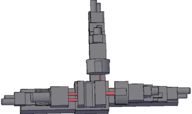
Figures 3 to 5 in Section 5 show an example of batch of three different parts.
Let us recall the introduced indexes for further presentation of parameters and decision variables:
– Index for reconfigurable machines k = 1,...,m, where m is the number of machines. – Index for parts: dD={1,2,…,d0}, where d0 is the number of types of parts. – Index for batches : =1,2,…,, where is the number of batches to be produced.
– Index for the positions of parts in sequence of each batch: =(1, 2, …,) where j{1,2,…,d0}, j=1,2,…, and is the number of parts processed in a sequence in batch = O.
Let Nd be the set of machining operations needed for machining of elements of dth part, dD={1,2,…,d 0} located on its nd sides and N , s=1, 2,…,nsd d, is a subset of operations for machining of elements of sth
side of the part d. The part d can be located at a machine in different orientations H(d) but elements of no more than one side can be processed by a machining module. Machining modules can be of 4 types: type
j=1 (from above), j=2 (from the left), j=3 (from behind), j=4 (from the right) and no more than 3 types of
machining modules can be installed at each machine. H(d) can be represented by a matrix of dimensions
rd x nd where hrs(d) is equal j, j=0,1,2,3,4, if the operations of N can be processed by machining sd
Let N be the set of all operations required for completing all considered parts, N= 0 1
d d N
d. Any operation
pN is characterized by the following parameters: the length (p) of the working stroke for operation p, the range [γ1(p),γ2(p)] of feasible values of feed rate defining cutting speed, and the set J(p) of types of possible machining modules for execution of operation p.
The considered optimization problem is to determine: – the number m of machines;
– the orientation Hdk of part dD at machine k, k = 1,...,m;
– the number bkj of machining modules of type j, j=1,…,4, that are installed at machine k, k=1,...,m;
– the set of machining operations Ndkjl from Nd, assigned to machining module l of type j at machine k,
dD, k = 1,...,m, j=1,...,4, l=1,...,bkj;
– the feed rate Гdkjl[max{γ1(u)|uNdkjl},min{γ2(u)|uNdkjl}] for execution of operations from Ndkjl, dD,
k=1,...,m, j=1,...,4, l=1,...,bkj.
Let Pdkj = (Pdkjl = (Ndkjl,Гdkjl)| l=1,...,bkj), Pdk = (Pdkj| j=1,…,4), Pd = ((Pdk, Hdk)| k = 1, ...,m), P = (Pd | dD).
P is a design decision.
The execution time tb(Pdkjl) of operations from Ndkjl with the feed rate
Гdkjl[max{γ1(p)|pNdkjl},min{γ2(p)|pNdkjl}] is equal to tb(Pdkjl) = L(Ndkjl)/Гdkjl +a, where
L(Ndkjl) = max{(p)| pNdkjl}, and a is an additional time for advance and disengagement of tools.
We assume that if the turret of type j is installed at machine k then the execution time of operations from
Ndkjl is equal to th(Pdkj) = gbkj +
kj
b l 1
tb(Pdkjl), j=1,…,4, where g is an additional time for one rotation of a
turret. If the spindle head is installed, then th(Pdkj) = tb(Pdkjl), j=1,…,4. If all Ndkjl are empty then
th(Pdkj) = 0. If bkj =1, then th(Pdkj) = tb(Pdkj1).
The execution time tp(Pdk) is defined as tp(Pdk) = r+ max{th(Pdkj)| j=1,…,4}, where r is an additional
time for part transportation and its location at a machine. Then the time T(P) of execution of all
corresponding operations for batch is defined as T(P)=
1 1 m O i max{tp(P(i,k)k)|k=1,,m} and the time T(P) for machining all the batches is equal to
1 T(P).
We assume that the given productivity is provided, if the total time T(P) does not exceed the available time T0.
Let Csm, Ctb, Cmm, Csb, and Cst be the relative costs for one machine, one turret, one machining module of
a turret, one spindle box, and one workhead with a single spindle, respectively. Then the cost C(bkj) for
performing set of operations Nkj by associated bkj machining modules can be assessed as follows:
C(bkj) = . 1 if , 1 | | and 1 if , 1 | | and 1 if , 0 if 0 1 1 kj kj mm tb kj kj sb kj kj st kj b b C C N b C N b C b
The machine cost Q(P) is calculated as the total cost of all equipment used:
1 1 1 1 1 4 1 0 ) , ( ) ( ) ( m k d d dk dk m k j kj smm C b C H H C P Q ,
where C(Hdk,Hdk+1) is the cost incurred by changing orientation of part d between stations k and k+1 and C(Hdk,Hdk+1)=0 if Hdk = Hdk+1 and C(Hdk,Hdk+1)= Cro, otherwise (Cro is the relative cost for reorientation).
The design decision P should satisfy the following constraints:
– precedence constraints which define time dependencies among operations;
– inclusion constraints which require to execute some pairs of operations from N at the same machine, by the same turret, by the same machining module or even by the same spindle;
– exclusion constraints which require to not assign some pairs of operations from N to the same machine, to the same turret, or to the same machining module;
– constraints on the maximal number m0 of machines and on the maximal number b0 of machining modules in a turret;
– constraints on feasible orientations of the part for processing each operation;
– the impossibility to perform operations from N at one machine by machining modules of sd
different types;
– productivity constraints to provide the required output (a time limit for total completion time). Precedence constraints are modelled by a directed graph GOR=(N,DOR): if an arc (p,q)DOR then operation
p has to be executed before operation q. It should be noted that if such operations p and q belong to
different sides of the part, then they cannot be executed at the same machine without violating the precedence constraint.
Inclusion constraints are represented by undirected graphs GSP=(N,ESP), GST=(N,EST), GSM=(N,ESM) and
GSS=(N,ESS): if there is an edge (p,q)ESS (or (p,q)ESM, or (p,q)EST, or (p,q)ESP), then operations p
and q must be executed by the same spindle (the same machining module, turret, at the same machine, respectively).
Exclusion constraints are represented by undirected graphs GDM=(N,EDM), GDT=(N,EDT), and
GDP=(N,EDP). If there is an edge (p,q)EDM (or (p,q)EDT), or (p,q)EDP)), then operations p and q
cannot be executed by the same machining module (turret, at the same machine, respectively).
4. MIP approach
In order to solve the considered problem, we developed a Mixed Integer Programming (MIP) model where the following notations are used:
Xpkjl decision variable which is equal to 1 if operation p is assigned to the lth machining module of
spindle head or turret of type j at station k, pN, k=1,…,m0, j=1,…,4, l=1,,b0
hrdk decision variable which is equal to 1 if orientation r is chosen for part d at station k, r=1,…,rd,
dD, k=1,…,m0
ds kj
Y auxiliary variable which is equal to 1 if at least one machining module of type j is installed at
station k for execution of operations from
N
sd , dD, s=1,…,nd, k=1,…,m0, j=1,…,4 dkj
Y auxiliary variable which is equal to 1 if at least one machining module of type j is installed at station k for execution of operations from Nd, dD, k=1,…,m0, j=1,…,4
Ykjl auxiliary variable which is equal to 1 if the lth machining module of type j is installed at station
k, k=1,…,m0, j=1,…,4, l=1,,b0
Ykjs auxiliary variable which is equal to 1 if the workhead with a single spindle of type j is installed at
station k, k=1,…,m0, j=1,…,4
Ykjb auxiliary variable which is equal to 1 if the spindle box of type j is installed at station k,
k=1,…,m0, j=1,…,4
Zk auxiliary variable which is equal to 1 if station k is used, k=1,…,m0
dkk+1 auxiliary variable which is equal to 1 if part d is reoriented between stations k and k+1, dD, k=1,…,m0-1
Fdkjl execution time for part d by l-th machining module of spindle head or turret type j at the k-th
machine
Fdk the execution time for part d at k-th machine
Fi total remaining processing time when processing of part i of -th batch is finished
i s
F total time of first i machines after the i-th turn of the conveyer for processing -th batch
i f
F total time of last i machines after the O+m0-i-th turn of the conveyer for processing -th batch number of cyclically repeating part sequences when all machines are occupied =(O
additional number of part sequences when all machines are occupied =mod(O-m0+1,) tpq minimal time necessary for the execution of operations p and q by the same machining module,
tpq = max((p), (q))/min(2(p),2(q))+a
M an upper bound on the maximal number of operations to be potentially assigned to one
machining module 0 max{ | 1, , }
1 d d s d d n s N M
The objective function can be expressed as follows:
Minimize 1 ( ( 2 ) 2 ) 4 1 1 0 0 kjs st kj mm tb m k j sb kjb m k k sm Z C Y C C Y C Y C
1 1 1 1 4 1 3 0 0 0 m k d D dkk ro m k j b l kjl mm Y C C (1)The following equations determine decision variables Xpkjl as well as auxiliary variables Ykjds, Ykjl, and Zk.
1 0 0 1 4 1 1 m k j n l Xpkjl ; pN (2) Xpkjl=0; j=1,…,4; jJ(p) (3) qkjl l l pkjl k k j b l pk jl X X X 1 1 ' ' 1 1 ' 4 1 1 ' '' 0 ; (p,q)DOR; k=1,…,m0; j=1,…,4; l=1,…,b0 (4) XpkjlXqkjl; {p,q}ESMESS; k=1,…,m0; j=1,…,4; l=1,…,b0 (5) 0 1 b l Xpkjl= 0 1 b l Xqkjl ; {p,q}EST; k=1,…,m0; j=1,…,4 (6) 4 1 1 0 j b l pkjl X = 4 1 1 0 j b l qkjl X ; {p,q}ESP; k=1,…,m0 (7) Xpkjl+Xqkjl1; {p,q}EDM; k=1,…,m0; j=1,…,4; l=1,…,b0 (8) 0 0 1 1 b l qkjl b l Xpkjl X +Ykj2 2; {p,q}EDT; k=1,…,m0; j=1,…,4 (9) 0 0 1 4 1 1 4 1 b l qkjl j b l pkjl j X X 1; {p,q}E DP; k=1,…,m0 (10) d s N p pkjl b l X 0 1 | d s N |Ykjds; Ykjds d s N p pkjl b l X 0 1 ; dD; s=1,…,n d; k=1,…,m0, j=1,…,4 (11)
4 1 1, j ds kj Y dD; s=1,…,nd; k=1,…,m0 (12) d n s ds kj Y 1 , 1 dD; k=1,…,m0; j=1,…,4 (13) Ykjl N p pkjl X ; N p pkjl X |N|Ykjl; k=1,…,m0; j=1,…,4; l=1,…,b0 (14) Ykjl Ykjl+1; k=1,…,m0; j=1,…,4; l=1,…,b0–1 (15) 4 1 1 j kj Y 3; 4 1 1 j kj Y 3Zk; Zk 4 1 1 j kj Y ; k=1,…,m0 (16) , 1 2 1 X Ykj MYkjs M p N pkj k=1,…,m0; j=1,…,4 (17) , 1 2 kjs kj kj kjb Y Y Y Y k=1,…,m0; j=1,…,4 (18) ZkZk-1; k=2,…,m0 (19)
Constraints (2) – (3) guarantee an assignment of each operation to exactly one machining module of compatible type. Precedence constraints, inclusion constraints for spindles, machining modules, turrets and machines as well as exclusion constraints for machining modules, turrets and machines are provided by (4) – (10) respectively. Constraints (11) – (12) prevent from an assignment of operations located at the same side of each part to machining modules of different types of the same machine. Constraints (13) – (19) define the configuration of machines, workheads with single spindle, spindle boxes, turrets, and corresponding machining modules. A workhead with single spindle is installed (Ykjs=1) if and only if
1 1
N
p Xpkj , Y
kj1=1, Ykjb=0 and Ykj2=0. If Ykj2=1 (a turret is installed), then Ykjb=0 and Ykjs=0.
Decision variables hrdk and auxiliary variables dkk+1 are defined by the following constraints: ds kj rdk Y h 1; r=1,…,rd; dD; k=1,…,m0; s=1,…,nd; j=1,…,4; jhrs(d) (20) 1 1 d r r rdk h ; dD; k=1,…,m0 (21) 1 1 1 1 r rdk r rdk r r dkk d d d rh rh r ; r rdk r rdk r r dkk d d d rh rh r 1 1 1 1 ; dD; k=1,…,m0-1 (22)
Constraints (20) – (21) defines the orientation of each part at each machine. Variables dkk+1 are equal to 0 if hrdk = hrdk+1 for all r=1,…,rd due to (22) and minimization of (1).
The required productivity is provided if the following constraints are satisfied: FdkjltppXpkjl; pNd; dD; k=1,…,m0; j=1,…4; l=1,…,b0 (23) Fdkjltpq(Xpkjl +Xqkjl – 1); p, qNd; dD; k=1,…,m0; j=1,…,4; l=1,…,b0 (24) Fdk 0 1 b l dkjl F +g(2Ykj2+ 0 3 b l kjl Y )+b0g(Ykjd–1); dD; k=1,…,m0; j=1,…,4 (25) i F (m0 i 1,k) k F +r; =1,…,; i=1,…, ; k=1,…,m0 (26) i s F Fk( ki, )+r; =1,…,; i=1,…,m0-1; k=1,…,i (27) i f F (O m0 i,k) k F +r; =1,…,; i=2,…,m0; k= i,,m0 (28) ) ( 0 0 2 1 1 1 1 1 m i i f m i i s i i i i F F F F T0 (29)
Constraints (21) – (22) calculate the execution time of the l-th machining module of type j at the k-th machine for processing part d. If a turret of type j with bkj machining modules is installed at the k-th
machine then: Fdk g b l d kjl b F kj
1 0due to (25) if at least one operation from Nd is executed by the turret
and Fdk =0, otherwise. If a spindle head of type j is installed at the k-th machine then Fdk Fkjd1.
Variables domains are defined as follows:
Xpkjl pN; k=1,…,m0; j=1,…,4; l=1,…,b0 (30) ds kj Y k=1,…,m0; dD; s=1,…,nd; j=1,…,4 (31) d kj Y k=1,…,m0; dD; j=1,…,4 (32) d kjl Y k=1,…,m0; j=1,…,4; l=1,…,b0; dD (33) Ykjl k=1,…,m0; j=1,…,4; l=1,…,b0 (34) Zk k=1,…,m0 (35) hrdk r=1,…,rd; dD; k=1,…,m0 (36) dkk+1 dD; k=1,…,m0-1 (37) d kjl F tkd k=1,…,mr 0; j=1,…,4; l=1,…,b0; dD (38)
d k F tkd r k=1,…,m0; dD (39) i F titi i=1,…, (40) i s F max{t(i,k)|k1,...,i}max{t (i,k)|k 1,...,i} k i=1,…,m0-1 (41) i f
F max{t(Oi,k)|k i,...,m0}max{tk(Oi,k)|k i,...,m0} i=2,…,m0 (42) where d t =min{(p)/2(p)+a+r| pNd}, } ,..., 1 | max{t ( , ) k m0 ti ik , ' 1 ' ' 1,' ' ' ' ' , 1 ' ' 0 )/ ( i i i i i i i T O t O t t and } ) , ( , 1 ,..., 1 , ,..., 1 | max{t i O m0 i k d tkd i . 5. A case study
In order to validate the developed model, it was used to design a flow line for machining 3 different parts (Fig. 3 to Fig. 5) in 2 batches with O1=34 and O2=68. The parameters of machining operations are given in Table 1. The operations to be executed for the first part are located on 4 different sides and those for the second and third parts are located on only 3 sides. The loading sequences of parts are {1,2} and {3}. Other parameters are: a = g = r = 0.1 min, Csm=20, Csh=4, Ctb=5, Cmm=2, Cro=0.5. The available time T0
is 384 min. The possible orientations of the parts are defined as follows:
H(1)= 1 1 2 1 1 4 1 1 1 1 1 4 1 1 1 4 1 4 1 1 , H(2)= 1 2 1 1 1 4 4 1 1 ,H(3)= 1 1 4 1 1 2 4 1 1 2 1 1 .
Fig.3. The first part to be machined
Fig.4. The second part to be machined
Fig.5. The third part to be machined H3 H4 H6 H5 H7 H8 H10 H9 H21 H22 H18 H16 H15 H17 H19 H20 H13 H3 H4 H6 H5 H7 H8 H10 H9 H16 H18 H15 H17 H4 H5 H8 H6 H7 H9 H11 H10 H13 H14 H16 H12 H15 H12 H11 H14
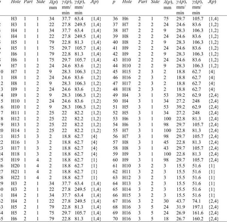
Table 1. Operations and their parameters p Hole Part Side (p)
mm γ1(p), mm/ min γ2(p), mm/ min
J(p) p Hole Part Side (p), mm γ1(p), mm/ min γ2(p), mm/ min J(p) 1 H3 1 1 34 37.7 63.4 {1,4} 36 H6 2 1 75 29.7 105.7 {1,4} 2 H3 1 1 22 27.8 249.5 {1,4} 37 H7 2 2 24 24.6 83.6 {1,2} 3 H4 1 1 34 37.7 63.4 {1,4} 38 H7 2 2 9 28.3 106.3 {1,2} 4 H4 1 1 22 27.8 249.5 {1,4} 39 H8 2 2 24 24.6 83.6 {1,2} 5 H5 1 1 79 22.8 81.3 {1,4} 40 H8 2 2 9 28.3 106.3 {1,2} 6 H5 1 1 75 29.7 105.7 {1,4} 41 H9 2 2 24 24.6 83.6 {1,2} 7 H6 1 1 79 22.8 81.3 {1,4} 42 H9 2 2 9 28.3 106.3 {1,2} 8 H6 1 1 75 29.7 105.7 {1,4} 43 H10 2 2 24 24.6 83.6 {1,2} 9 H7 1 2 24 24.6 83.6 {1,2} 44 H10 2 2 9 28.3 106.3 {1,2} 10 H7 1 2 9 28.3 106.3 {1,2} 45 H15 2 3 2 18.8 62.7 {4} 11 H8 1 2 24 24.6 83.6 {1,2} 46 H16 2 3 2 18.8 62.7 {4} 12 H8 1 2 9 28.3 106.3 {1,2} 47 H17 2 3 2 18.8 62.7 {4} 13 H9 1 2 24 24.6 83.6 {1,2} 48 H18 2 3 2 18.8 62.7 {4} 14 H9 1 2 9 28.3 106.3 {1,2} 49 H4 3 1 53 39.2 62.9 {2,4} 15 H10 1 2 24 24.6 83.6 {1,2} 50 H4 3 1 34 27.2 248 {2,4} 16 H10 1 2 9 28.3 106.3 {1,2} 51 H5 3 1 53 39.2 62.9 {2,4} 17 H11 1 2 25 22 82.2 {1,2} 52 H5 3 1 34 27.2 248 {2,4} 18 H12 1 2 25 22 82.2 {1,2} 53 H6 3 1 100 22.8 81.3 {2,4} 19 H13 1 2 25 22 82.2 {1,2} 54 H6 3 1 98 29.7 105.7 {2,4} 20 H14 1 2 25 22 82.2 {1,2} 55 H7 3 1 100 22.8 81.3 {2,4} 21 H15 1 3 2 18.8 62.7 {4} 56 H7 3 1 98 29.7 105.7 {2,4} 22 H16 1 3 2 18.8 62.7 {4} 57 H8 3 1 45 22.8 81.3 {2,4} 23 H17 1 3 2 18.8 62.7 {4} 58 H8 3 1 43 29.7 105.7 {2,4} 24 H18 1 3 2 18.8 62.7 {4} 59 H9 3 1 100 22.8 81.3 {2,4} 25 H19 1 4 2 18.8 62.7 {1} 60 H9 3 1 98 29.7 105.7 {2,4} 26 H20 1 4 2 18.8 62.7 {1} 61 H10 3 2 3 15.5 51.6 {1} 27 H21 1 4 2 18.8 62.7 {1} 62 H11 3 2 3 15.5 51.6 {1} 28 H22 1 4 2 18.8 62.7 {1} 63 H12 3 2 3 15.5 51.6 {1} 29 H3 2 1 34 37.7 63.4 {1,4} 64 H13 3 2 3 15.5 51.6 {1} 30 H3 2 1 22 27.8 249.5 {1,4} 65 H14 3 2 3 15.5 51.6 {1} 31 H4 2 1 34 37.7 63.4 {1,4} 66 H15 3 2 3 15.5 51.6 {1} 32 H4 2 1 22 27.8 249.5 {1,4} 67 H16 3 2 30 43.7 74.1 {2,4} 33 H5 2 1 79 22.8 81.3 {1,4} 68 H16 3 5 24 31.9 197.1 {2,4} 34 H5 2 1 75 29.7 105.7 {1,4} 69 H16 3 5 24 26.9 161.6 {2,4} 35 H6 2 1 79 22.8 81.3 {1,4} 70 H16 3 5 18 26.7 160.2 {2,4}
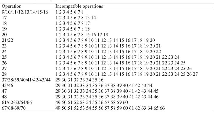
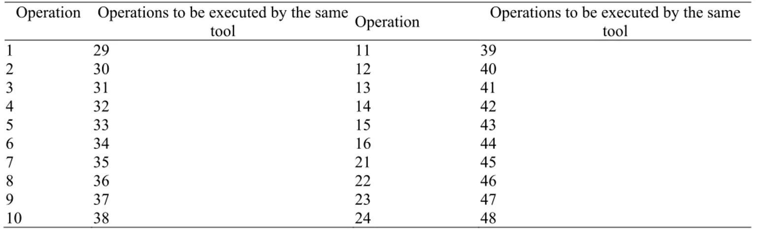
Precedence constraints, exclusion constraints for machining modules, turrets and machines are presented in Tables 2, 3, 4, and 5, respectively. Inclusion constraints for machines, turrets and machining modules are given in Tables 6, 7 and 8. Operations to be executed by the same spindle are presented in Table 9.
Table 2. Precedence constraints
Operation Predecessors Operation Predecessors
2 1 3 29 31 40 9 11 13 15 37 39 41 43 4 1 3 29 31 42 9 11 13 15 37 39 41 43 6 5 7 33 35 44 9 11 13 15 37 39 41 43 8 5 7 33 35 50 49 51 10 9 11 13 15 37 39 41 43 52 49 51 12 9 11 13 15 37 39 41 43 54 53 55 59 14 9 11 13 15 37 39 41 43 56 53 55 59 16 9 11 13 15 37 39 41 43 58 57 30 1 3 29 31 60 53 55 59 32 1 3 29 31 68 67 34 5 7 33 35 69 68 36 5 7 33 35 70 69 38 9 11 13 15 37 39 41 43
Table 3. Incompatibility of operations in machining modules Operation Incompatible operations
9/10/11/12/13/14/15/16 1 2 3 4 5 6 7 8 17 1 2 3 4 5 6 7 8 13 14 18 1 2 3 4 5 6 7 8 17 19 1 2 3 4 5 6 7 8 18 20 1 2 3 4 5 6 7 8 15 16 17 19 21/22 1 2 3 4 5 6 7 8 9 10 11 12 13 14 15 16 17 18 19 20 23 1 2 3 4 5 6 7 8 9 10 11 12 13 14 15 16 17 18 19 20 21 24 1 2 3 4 5 6 7 8 9 10 11 12 13 14 15 16 17 18 19 20 22 25 1 2 3 4 5 6 7 8 9 10 11 12 13 14 15 16 17 18 19 20 21 22 23 24 26 1 2 3 4 5 6 7 8 9 10 11 12 13 14 15 16 17 18 19 20 21 22 23 24 25 27 1 2 3 4 5 6 7 8 9 10 11 12 13 14 15 16 17 18 19 20 21 22 23 24 25 26 28 1 2 3 4 5 6 7 8 9 10 11 12 13 14 15 16 17 18 19 20 21 22 23 24 25 26 27 37/38/39/40/41/42/43/44 29 30 31 32 33 34 35 36 45/46 29 30 31 32 33 34 35 36 37 38 39 40 41 42 43 44 47 29 30 31 32 33 34 35 36 37 38 39 40 41 42 43 44 45 48 29 30 31 32 33 34 35 36 37 38 39 40 41 42 43 44 46 61/62/63/64/66 49 50 51 52 53 54 55 56 57 58 59 60 67/68/69/70 49 50 51 52 53 54 55 56 57 58 59 60 61 62 63 64 65 66
Table 4. Incompatibility of operations in turrets
Operation Incompatible operations
9/10/11/12/13/14/15/16/17/18/19/20 1 2 3 4 5 6 7 8 21/22/23/24 1 2 3 4 5 6 7 8 9 10 11 12 13 14 15 16 17 18 19 20 25/26/27/28 1 2 3 4 5 6 7 8 9 10 11 12 13 14 15 16 17 18 19 20 21 22 23 24 37/38/39/40/41/42/43/44 29 30 31 32 33 34 35 36 45/46/47/48 29 30 31 32 33 34 35 36 37 38 39 40 41 42 43 44 61/62/63/64/65/66 49 50 51 52 53 54 55 56 57 58 59 60 67/68/69/70 49 50 51 52 53 54 55 56 57 58 59 60 61 62 63 64 65 66
Table 5. Incompatibility of operations in machines
Operation Incompatible operations
1/2/3/4/5/6/7/8 21 22 23 24
17/18/19/20 25 26 27 28
Table 6. Operations to be assigned to the same machine Operation Operations to be executed at the same
machine Operation
Operations to be executed at the same machine
49 51 53 55 57 59 50 52 54 56 58 60
Table 7. Operations to be assigned to the same turret Operation Operations to be executed by the same
turret Operation
Operations to be executed by the same turret
25 26 27 28 67 68 69 70
Table 8. Operations to be assigned to the same machining module Operation Operations to be executed by the same
machining module Operation
Operations to be executed by the same machining module 1 3 33 35 5 7 34 36 6 8 37 39 41 43 9 11 13 15 49 51 17 19 53 55 59 18 20 54 56 60 29 31
Table 9. Operations to be executed by the same spindle Operation Operations to be executed by the same
tool Operation
Operations to be executed by the same tool 1 29 11 39 2 30 12 40 3 31 13 41 4 32 14 42 5 33 15 43 6 34 16 44 7 35 21 45 8 36 22 46 9 37 23 47 10 38 24 48
Solver CPLEX 12.2 was used to solve the corresponding problems (1) – (42) for b0=4 and m0=2, 3, 4, 5 on PC Intel Pentium (2.40 Ghz, 4 Gb RAM). The obtained results are presented in Table 10.
Table 10. Results of optimization
m0 Number of variables Number of constraints Solution time, s
2 1639 49700 8.18
3 2458 74553 20.13
4 3277 99406 40.51
In all obtained solutions the flow line consists of 2 machines and 2 turrets should be installed at each machine but the assignment of operations to machining modules is quite different. The obtained optimal solution for m0=5 and its characteristics are presented in Tables 11 and 12. The total cost Q(P) is equal to 2Csm+0Csh+4Ctb+12Cmm+3Cro5=85.5. In this case p1=32, p2=64, 1 =2 =0. The total time T(P) is equal to 32(2.46+2.46)+1.03+2.46+2.46+2.46+2.46+64(3.02)+ 3.02+3.02+3.02+3.02+1.96= 375.63 min.
Table 11. An optimal solution
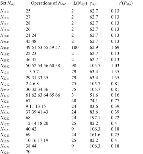
Set Ndkjl Operations of Ndkjl L(Ndkjl) γdkjl tb(Pdkjl) N1111 25 2 62.7 0.13 N1112 27 2 62.7 0.13 N1113 28 2 62.7 0.13 N1114 26 2 62.7 0.13 N1141 21 24 2 62.7 0.13 N2141 45 48 2 62.7 0.13 N3141 49 51 53 55 59 57 100 62.9 1.69 N1142 22 23 2 62.7 0.13 N2142 46 47 2 62.7 0.13 N3142 50 52 54 56 60 58 98 105.7 1.03 N1211 1 3 5 7 79 63.4 1.35 N2211 29 31 33 35 79 63.4 1.35 N1212 2 4 6 8 75 105.7 0.81 N2212 30 32 34 36 75 105.7 0.81 N3212 61 62 63 64 65 66 3 51.6 0.16 N3221 67 40 74.1 0.77 N1222 9 11 13 15 24 83.6 0.39 N2222 37 39 41 43 24 83.6 0.39 N3222 68 24 197.1 0.22 N1223 12 14 18 20 25 82.2 0.4 N2223 40 42 9 106.3 0.18 N3223 69 24 161.6 0.25 N1224 10 16 17 19 25 82.2 0.4 N2224 38 44 9 106.3 0.18 N3224 70
Table 12. Characteristics of the solution Machine k tp(P 1k) tp(P2k) tp(P3k) H1k H2k H3k 1 1.03 0.56 3.02 -1,-1,4,1 -1,1,4 4,-1,-1 2 2.46 2.46 1.96 1,2,-1,-1 1,2,-1 -1,1,2 3 0 0 0 - - - 4 0 0 0 - - - 5 0 0 0 - - -
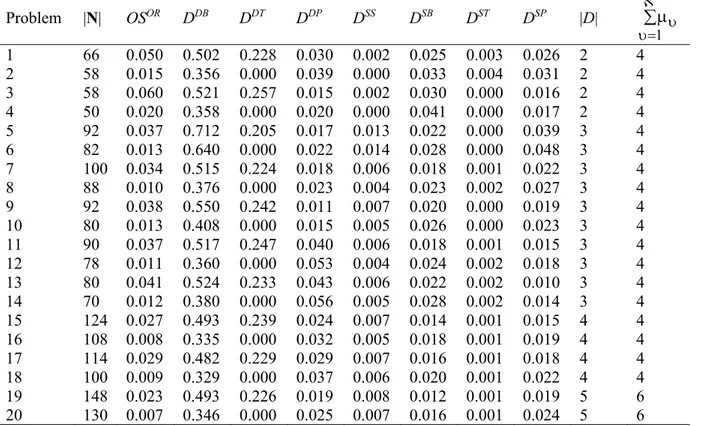
The proposed approach was also tested on 20 industrial examples with ||=2. The proprieties of these instances are given in Table 9 where OSOR is the order strength of the precedence constraints (the ratio
between the number of arcs in the closure of GOR and the number of arcs in the complete digraph with the
same number of vertices. Densities of other constraints (DDM, DDT, DDP, DSS, DSM, DST, and DSP) are
Table 9. The proprieties of the industrial examples Problem |N| OSOR DDB DDT DDP DSS DSB DST DSP |D| 1 1 66 0.050 0.502 0.228 0.030 0.002 0.025 0.003 0.026 2 4 2 58 0.015 0.356 0.000 0.039 0.000 0.033 0.004 0.031 2 4 3 58 0.060 0.521 0.257 0.015 0.002 0.030 0.000 0.016 2 4 4 50 0.020 0.358 0.000 0.020 0.000 0.041 0.000 0.017 2 4 5 92 0.037 0.712 0.205 0.017 0.013 0.022 0.000 0.039 3 4 6 82 0.013 0.640 0.000 0.022 0.014 0.028 0.000 0.048 3 4 7 100 0.034 0.515 0.224 0.018 0.006 0.018 0.001 0.022 3 4 8 88 0.010 0.376 0.000 0.023 0.004 0.023 0.002 0.027 3 4 9 92 0.038 0.550 0.242 0.011 0.007 0.020 0.000 0.019 3 4 10 80 0.013 0.408 0.000 0.015 0.005 0.026 0.000 0.023 3 4 11 90 0.037 0.517 0.247 0.040 0.006 0.018 0.001 0.015 3 4 12 78 0.011 0.360 0.000 0.053 0.004 0.024 0.002 0.018 3 4 13 80 0.041 0.524 0.233 0.043 0.006 0.022 0.002 0.010 3 4 14 70 0.012 0.380 0.000 0.056 0.005 0.028 0.002 0.014 3 4 15 124 0.027 0.493 0.239 0.024 0.007 0.014 0.001 0.015 4 4 16 108 0.008 0.335 0.000 0.032 0.005 0.018 0.001 0.019 4 4 17 114 0.029 0.482 0.229 0.029 0.007 0.016 0.001 0.018 4 4 18 100 0.009 0.329 0.000 0.037 0.006 0.020 0.001 0.022 4 4 19 148 0.023 0.493 0.226 0.019 0.008 0.012 0.001 0.019 5 6 20 130 0.007 0.346 0.000 0.025 0.007 0.016 0.001 0.024 5 6
The experiments were carried out for two variants of each problem that differed in matrices H(d) and sets
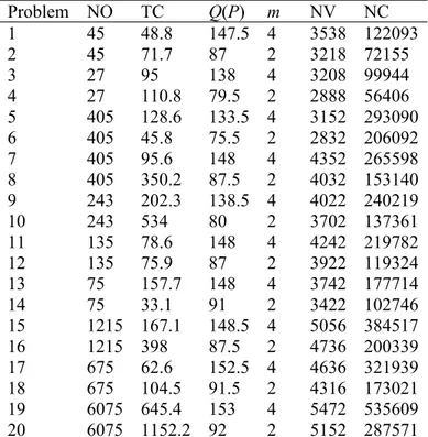
J(p). The results are presented in Tables 10 and 11 where NO is the number of rows of a matrix H of possible orientations of all parts, TC is the calculation time in seconds, NV and NC are the numbers of variables and constraints in MIP formulations, respectively. H is built on the base of matrices H(d) and takes also into account constraints DSS and DSM.
Table 10. The results for the first variant
Problem NO TC Q(P) m NV NC 1 20 10.9 158.5 4 3513 122608 2 16 16.4 119.5 3 3188 72585 3 10 14.4 143.5 4 3183 100419 4 8 13.6 103 3 2858 56796 5 125 10.6 136 4 3112 293550 6 48 14.2 96.5 3 2772 206452 7 100 16.9 159.5 4 4307 266213 8 64 69.2 120.5 3 3977 153665 9 50 24.8 144.5 4 3977 240794 10 32 24.3 104 3 3647 137846 11 40 20.2 159 4 4212 220392 12 32 44.2 119.5 3 3887 119849 13 40 40.1 148.5 4 3732 178124 14 24 8.3 91 2 3402 103066 15 200 29.2 160 4 5006 385227 16 128 64.6 120.5 3 4676 200959 17 200 25.2 160 4 4606 322529 18 96 43.1 120 3 4271 173516 19 1000 47.8 161 4 5422 536299 20 384 76.6 121 3 5082 288161
Table 11. The results for the second variant Problem NO TC Q(P) m NV NC 1 45 48.8 147.5 4 3538 122093 2 45 71.7 87 2 3218 72155 3 27 95 138 4 3208 99944 4 27 110.8 79.5 2 2888 56406 5 405 128.6 133.5 4 3152 293090 6 405 45.8 75.5 2 2832 206092 7 405 95.6 148 4 4352 265598 8 405 350.2 87.5 2 4032 153140 9 243 202.3 138.5 4 4022 240219 10 243 534 80 2 3702 137361 11 135 78.6 148 4 4242 219782 12 135 75.9 87 2 3922 119324 13 75 157.7 148 4 3742 177714 14 75 33.1 91 2 3422 102746 15 1215 167.1 148.5 4 5056 384517 16 1215 398 87.5 2 4736 200339 17 675 62.6 152.5 4 4636 321939 18 675 104.5 91.5 2 4316 173021 19 6075 645.4 153 4 5472 535609 20 6075 1152.2 92 2 5152 287571
The obtained results show that the tested industrial problems could be solved to optimality in reasonable time. However, the complexity of the problem and the time required to solve it strongly depends on the density of inclusion and exclusion constraints which in fine define the number of possible solutions.
Conclusions
In this paper, we developed a new mathematical model for the cost optimization problem in the design of machining flow lines composed of reconfigurable machines and used for batch production. This new model includes the definition of precedence, exclusion and inclusion constraints among operations and different types of equipment, such as machining modules, turrets, spindle boxes and workheads with single spindles. The configuration of the line is decided by optimizing the assignment of operations to the pieces of equipment while satisfying technical and technological constraints as well as the required final completion time.
The developed model is general and can be applied to different reconfigurable manufacturing systems (RMS) used in machining industry. The proposed model has been successfully validated on industrial case studies. The obtained results show that it can be used in practice for designing RMS for variable batches of parts required in low volume. In particular, the solution time for finding optimal solutions for industrial problems is acceptable. Therefore, the use of the developed model may help designers to evaluate quickly different design configurations and the investment costs required. Thus, the total cost and design time can be substantially reduced. The future research will include the integration of environmental factors into the considered problem. Despite of the fact that the investment cost is still
important for decision makers in industry, solutions can be also compared on the basis of their environmental indicators such as energy consumption, waste generation, options available for the end of life treatment. However, an important effort will be needed to properly model these environmental indicators.
Acknowledgements: This work was partially supported by the region Pays de la Loire (France).
References
Abbasi M, Houshmand M. Production planning of reconfigurable manufacturing systems with stochastic demands using Tabu search. Int J Manuf Technol Manage, 2009; 17(1-2):125–48.
Abbasi M, Houshmand D. Production planning and performance optimization of reconfigurable manufacturing systems using genetic algorithm. Int J Adv Manuf Technol, 2011; 54(1-4): 373–92.
Ashraf M, Hasan F. Configuration selection for a reconfigurable manufacturing flow line involving part production with operation constraints. Int J Adv Manuf Technol, 2018; 98(5-8), 2137–56.
Andresen AL, Brunoe TD, Nielsen K. Reconfigurable manufacturing on multiple levels: literature review and research directions. In: Advances in Production Management Systems: Innovative Production Management towards Sustainable Growth. IFIP conference; Springer; 2015. pp. 266–273.
Andersen AL, Nielsen K, Brunoe TD. Prerequisites and barriers for the development of reconfigurable manufacturing systems for high speed ramp-up. Procedia CIRP, 2016; 51: 7–12.
Andersen AL, Brunoe TD, Nielsen K, Rosio C. Towards a generic design method for reconfigurable manufacturing systems: analysis and synthesis of current design methods and evaluation of supportive tools. J Manuf Syst, 2017; 42: 179–95.
Battaïa O., Dolgui A., Guschinsky N. Decision support for design of reconfigurable rotary machining systems for family part production. Int J Prod Res, 2017; 55(5): 1368–1385.
Bensmaine A, Dahane M, Benyoucef L. A non-dominated sorting genetic algorithm based approach for optimal machines selection in reconfigurable manufacturing environment. Comput Ind Eng, 2013; 66(3): 519–24.
Bortolini M, Galizia FG, Mora C. Reconfigurable manufacturing systems: Literature review and research trend. J Manuf Syst, 2018; 49: 93–106.
Brahimi N, Dolgui A, Gurevsky E, Yelles-Chaouche AR. A literature review of optimization problems for reconfigurable manufacturing systems. IFAC PapersOnline, 2019. to appear
Buer S-V, Strandhagen JO, Chan FTS. The link between Industry 4.0 and lean manufacturing: mapping current research and establishing a research agenda. Int J Prod Res, 2018; 56(8): 2924-40.
Dolgui A, Levin G, Rozin B. Optimisation of the aggregation and execution rates for intersecting operation sets: an example of machining process design. Int J Prod Res, 2019; doi.org/10.1080/00207543.2019.1629668
Dou JP, Dai XZ, Meng ZD. Configuration selection of reconfigurable manufacturing system based on hybrid analytical hierarchy process. Comput Integr Manuf Syst, 2007; 13(7): 1360-66.
Dou JP, Dai XZ, Meng ZD. Optimisation for multi-part flow-line configuration of reconfigurable manufacturing systems using GA. Int J Prod Res, 2010; 48(14): 4071–100.
Dou J, Li J, Su C. Bi-objective optimization of integrating configuration generation and scheduling for reconfigurable flow lines using NSGA-II. Int J Adv Manuf Technol, 2016; 86(5-8): 1945–62.
Farid AM. Measures of reconfigurability and its key characteristics in intelligent manufacturing systems. J Intell Manuf, 2017; 28 (2), 353–369.
Goyal KK, Jain PK, Jain M. Optimal configuration selection for reconfigurable manufacturing system using NSGA II and TOPSIS. Int J Prod Res, 2012; 50(15): 4175–91.
Goyal KK, Jain PK, Jain M. A novel methodology to measure the responsiveness of RMTs in reconfigurable manufacturing system. J Manuf Syst, 2013; 32(4): 724–30.
Haddou-Benderbal H, Dahane M, Benyoucef L. Flexibility-based multi-objective approach for machine selection in reconfigurable manufacturing system (RMS) design under unavailability constraints. Int J Prod Res, 2017; 55(20): 6033–51.
Huettemann G, Gaffry C, Schmitt RH. Adaptation of reconfigurable manufacturing systems for industrial assembly—review of flexibility paradigms, concepts and outlook. Procedia CIRP, 2015; 52: 112–7. Koren Y, Heisel U, Jovane F, Moriwaki T, Pritschow G, Ulsoy G, et al. Reconfigurable manufacturing systems. CIRP annals—manufacturing technology, 1999; 48(2): 527–40.
Koren Y, Shpitalni M. Design of reconfigurable manufacturing systems. J Manuf Syst, 2010; 29(4): 130– 41.
Koren Y, Wang W, Gu X. Value creation through design for scalability of reconfigurable manufacturing systems. Int J Prod Res, 2017; 55(5):1227-1242.
Liao Y, Deschamps F, de Freitas Rocha Loures R, Pierin Ramos L.F. Past, present and future of Industry 4.0 - a systematic literature review and research agenda proposal. Int J Prod Res, 2017; 55(12): 3609-29. Moghaddam, S., Houshmand, M., and Valilai, O. Configuration design in scalable reconfigurable manufacturing systems (RMS) a case of single-product flow line (SPFL). Int J Prod Res, 2017; 56(11), 3932–54.
Renzi C, Leali F, Cavazzuti M, Andrisano AO. A review on artificial intelligence applications to the optimal design of dedicated and reconfigurable manufacturing systems. Int J Adv Manuf Technol, 2014; 72(1–4): 403–418.
Rosio C, Safsten K. Reconfigurable production system design—theoretical and practical challenges. J Manuf Technol Mngmt, 2013; 24(7): 998–1018.
Saxena LK, Jain PK. A model and optimisation approach for reconfigurable manufacturing system configuration design. Int J Prod Res, 2012; 50(12): 3359–81.
Singh A, Gupta S, Asjad M, Gupta P. Reconfigurable manufacturing systems: journey and the road ahead. Int J Syst Assur Eng Mngmt, 2017; 8(2): 1849–1857.
Son SY, Lennon Olsen T, Yip-Hoi D. An approach to scalability and line balancing for reconfigurable manufacturing systems. Integr Manuf Syst, 2001; 12(7): 500–11.
Spicer P, Yip-Hoi D, Koren Y. Scalable reconfigurable equipment design principles. Int J Prod Res, 2005; 43(22): 4839–52.
Wang W, Koren Y. Scalability planning for reconfigurable manufacturing systems. J Manuf Syst, 2012; 31(2): 83–91.
Xiaobo Z, Jiancai W, Zhenbi L. A stochastic model of a reconfigurable manufacturing system. Part 1: a framework. Int J Prod Res, 2000; 38(10): 2273–85.
Xiaobo Z, Wang J, Luo Z. A stochastic model of a reconfigurable manufacturing system. Part 2: optimal configurations. Int J Prod Res, 2000; 38(12): 2829–42.
Xiaobo Z, Wang J, Luo Z. A stochastic model of a reconfigurable manufacturing system. Part 3: optimal selection policy. Int J Prod Res, 2001; 39(4): 747–58.
Xiaobo Z, Wang J, Luo Z. A stochastic model of a reconfigurable manufacturing system. Part 4: performance measure. Int J Prod Res, 2001; 39(6): 1113–26.
Xu LD, Xu EL, Li L. Industry 4.0: state of the art and future trends. Int J Prod Res, 2018; 56(8): 2941-62. Yin Y, Stecke KE, Li D. The evolution of production systems from Industry 2.0 through Industry 4.0. Int J Prod Res, 2018; 56(1-2): 848-861.
Youssef AM, ElMaraghy HA. Modelling and optimization of multiple-aspect RMS configurations. Int J Prod Res, 2006; 46(22): 4929–58.
Youssef AM, ElMaraghy HA. Optimal configuration selection for reconfigurable manufacturing systems. Int J Flex Manuf Syst, 2007; 19(2): 67–106.
Youssef AM, ElMaraghy HA. Availability consideration in the optimal selection of multiple-aspect RMS configurations. Int J Prod Res, 2008; 46(21): 5849–82.