HAL Id: hal-02946881
https://hal.telecom-paris.fr/hal-02946881
Submitted on 23 Sep 2020
HAL is a multi-disciplinary open access
archive for the deposit and dissemination of
sci-entific research documents, whether they are
pub-L’archive ouverte pluridisciplinaire HAL, est
destinée au dépôt et à la diffusion de documents
scientifiques de niveau recherche, publiés ou non,
Slim Essid, Pierre Leveau, Gael Richard, Laurent Daudet, Bertrand David
To cite this version:
Slim Essid, Pierre Leveau, Gael Richard, Laurent Daudet, Bertrand David. On the usefulness of
differentiated transient/steady-state processing in machine recognition of musical instruments. AES
118th convention, May 2005, Barcelona, Spain. �hal-02946881�
Audio Engineering Society
Convention Paper
Presented at the 118th Convention 2005 May 28–31 Barcelona, Spain
This convention paper has been reproduced from the author’s advance manuscript, without editing, corrections, or consideration by the Review Board. The AES takes no responsibility for the contents. Additional papers may be obtained by sending request and remittance to Audio Engineering Society, 60 East 42nd Street, New York, New York 10165-2520, USA; also see www.aes.org. All rights reserved. Reproduction of this paper, or any portion thereof, is not permitted without direct permission from the Journal of the Audio Engineering Society.
On the usefulness of differentiated
transient/steady-state processing in machine
recognition of musical instruments
Slim ESSID1, Pierre LEVEAU1,2, Ga¨el RICHARD1, Laurent DAUDET2, and Bertrand DAVID1
1
GET - ENST (T´el´ecom Paris) - TSI, 46, rue Barrault - 75634 Paris Cedex 13 - FRANCE
2
Laboratoire d’Acoustique Musicale, 11 rue de Lourmel, 75015 Paris
Correspondence should be addressed to Slim ESSID (slim.essid@enst.fr)
ABSTRACT
This paper addresses the usefulness of the segmentation of musical sounds into transient/non-transient parts for the task of machine recognition of musical instruments. We put into light the discriminative power of the attack-transient segments on the basis of objective criteria, consistent with the well-known psychoacoustics findings. The sound database used is composed of real-world mono-instrument phrases. Moreover, we show that, paradoxically, it is not always optimal to consider such a segmentation of the audio signal in a machine recognition system for a given decision window. Our evaluation exploits efficient automatic segmentation techniques, a wide variety of signal processing features as well as feature selection algorithms and support vector machine classification.
1. INTRODUCTION
The attack and end transients of music notes carry a significant part of the information for musical instrument identification, as evidenced by music cognition and music acoustics studies [1, 2]. It is known that information about the production mode of the sound is essentially located at the beginning and at the end of the notes, like breath impulsions for the wind instruments, bow strokes for the bowed
strings, or plucking or hammering for percussive pitched instruments (for example piano and guitar). Additionally, music cognition experiments have shown that features related to the beginning of music notes (for example attack-time [2]) can help humans to discriminate different instrument notes.
For machine recognition tasks, signal processing features extracted from the attack transients (such
as crest factor, onset duration) have also proved to be efficient for instrument family identification in previous work on isolated notes [3]. However, performing reliable extraction of such features on mono-instrument phrases in real playing conditions is not straightforward. In fact, the state-of-the-art approaches of automatic music instrument recognition on solo performances are based on a cutting of the signal into short signal windows (about 30ms), and they do not differentiate the transient and steady-state windows. Therefore, since non-transient segments are usually much longer than transient ones, the information carried by the transients gets diluted over the entire signal, hence its impact on the final classification decision becomes weak.
Our study considers a differentiated processing on the transient and non-transient parts of the musical phrases. It assumes that we have at hand at least one algorithm that performs automatic segmen-tation of the signal, with an estimated error rate. Then, adapted features can be selected for each part.
We thus show, using class-separability criteria and recognition accuracy measures, that attack transient segments of the musical notes are more informative than other segments for instrument classification . Subsequently, we discuss the efficiency of such a seg-mentation in the perspective of developing a realistic machine recognition system.
2. SIGNAL SEGMENTATION
The signal analysis is based on 32-ms constant-length windows, with a 50%-overlap. After segmen-tation, each window is assigned to one of the follow-ing two categories: transient or non-transient. Two types of transient/non-transient segmentation are performed. The first type is based on an onset detector: when an onset is detected, a fixed num-ber of windows including and following the onset are considered as transient. The second type in-volves a continuous transientness criterion: windows for which this criterion exceeds a fixed threshold are considered as transient. The next two sections (2.1 and 2.2) describe these two methods in detail.
2.1. Fixed-duration transient annotation based on onset detection
2.1.1. Onset Detection Algorithm
The automatic onset detection is based on a detec-tion funcdetec-tion that uses a spectral difference, tak-ing the phase increment into account. The origi-nal method was introduced in [4]. It is based on the computation of a prediction error. If the signal is composed of stationary sinusoids, the first-order prediction of the Discrete Fourier Transform (DFT) Xk,n, of the signal x at frequency k and time n is:
ˆ
Xk,n = |Xk,n−1|ej(2φk,n−1−φk,n−2)
where φk,n is the time-unwrapped phase of Xk,n.
When an onset occurs, there is a break in the pre-dictability, and therefore a peak in the prediction error. We thus define the function ρ:
ρ(n) = ΣK
k=1| ˆXk,n− Xk,n|
that exhibits peaks at onset locations. However, when evaluating this detection function on real sounds, we find that these peaks occur sometimes late with respect to the note onset times, because of too long raising times of the function peaks. Al-though the onset is detected, the peak is located at the maximum spectral difference and not at the true onset time. Thus, we perform an additional opera-tion to sharpen the peaks of the detecopera-tion funcopera-tion ρ: a derivation (noted ∆) followed by a rectification:
γ(n) = max({∆(ρ(n)), 0})
Onsets are then extracted by peak-picking the new detection function γ, called Delta Complex Spectral Difference. A peak is selected if it is over a threshold δ(n), computed dynamically:
δ(n) = δstatic+ λ ∗ median(γ(n − M )), ..., γ(n + M ))
2.1.2. Onset Detection Evaluation
The above onset detection algorithm was compared to other standard onset detection algorithms, such as Spectral Difference (amplitude or complex do-main) and Phase Deviation [5]. It has also been eval-uated on a database of solo instrument recordings,
Essid et al. transient/steady-state segments in instrument recognition
manually annotated and cross-validated [6]. On the Receiver Operating Characteristic curves1 (Figure
1), the Delta Complex Spectral Difference shows a significant improvement in comparison to the other ones (its ROC curve is constantly over all the other ones). 10 20 30 40 50 60 70 20 30 40 50 60 70 80 90 100 False Detections [%] Good Detections [%] ROC Curve
Complex Spectral Difference Phase Deviation Spectral Difference Delta Complex Spectral Difference
Fig. 1: ROC Curves of the detection functions. (square): Complex Domain Spectral Difference, (plus): Phase Deviation, (circle): Spectral Differ-ence, (star): Delta Complex Spectral Difference 2.2. Transientness criterion
One of the main limitations of the system described above is that it assumes that all transient regions have the same length. Obviously, this is overly sim-plified when the signals considered range from per-cussive (that have very sharp attack transients) to string or wind instruments (that can have very long attack durations). Therefore, a more signal-adaptive algorithm has been developed, based on the contin-uous transientness criterion introduced by Goodwin in [7]. Like most onset detection algorithms, it is based on a spectral difference, with some adaption to the signal level. Given f the spectral flux func-tion:
f(n) = ΣK
k=1(|Xk,n| − |Xk,n−1|),
the following operation is performed:
1
good detections as a function of false alarms
if(f [n] > βn−1)
βn= f [n]
else
βn= αβn−1withα < 1
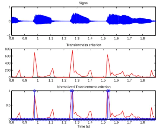
α must be set close to 1, and β initialized to the theoretical or empirical maximum of f . Figure 2 shows the adaption provided by this operation. The windows for which the criterion β remains over a fixed threshold are considered as transient windows.
0.8 0.9 1 1.1 1.2 1.3 1.4 1.5 1.6 1.7 1.8 −1 0 1 Signal 0.8 0.9 1 1.1 1.2 1.3 1.4 1.5 1.6 1.7 1.8 0 200 400 600 800 Transientness criterion 0.8 0.9 1 1.1 1.2 1.3 1.4 1.5 1.6 1.7 1.8 0 0.5 1
Normalized Transientness criterion
Time [s]
Fig. 2: Transientness Criterion. top: original signal (trumpet sample), middle: transientness criterion, bottom: normalized transientness criterion, circles at 1 indicate transient windows
2.3. A priori comparison of the segmentation methods
Once the two types of segmentation are performed, coincidence between the segmentations can be eval-uated. Since we lack a ground-truth for the tran-sientness, we can only provide this indication on the robustness of our segmentation with respect to the employed method.
For a nearly equal numbers of transient windows de-tected by both methods, we found that about 40% of each set of transient windows were common. For a random segmentation, the coincidence is about 7%. These quantities show that, although significantly correlated, the two methods are far from giving the same results. This means that results obtained only on transient windows may vary according to the cho-sen segmentation method.
AES 118th
Convention, Barcelona, Spain, 2005 May 28–31 Page 3 of 10
3. FEATURE EXTRACTION AND SELECTION
3.1. Feature extraction
A wide selection of more than 300 signal processing features is considered including some of the MPEG-7 descriptors. They are briefly described hereafter. Interested readers are referred to [8] for more de-tailed description.
3.1.1. Temporal features
• Autocorrelation Coefficients were reported to be useful in [9]; they represent the “signal spec-tral distribution in the time domain”.
• Zero Crossing Rates (ZCR) are computed over short windows and long windows; they can dis-criminate periodic signals (small ZCR values) from noisy signals (high ZCR values).
• Local temporal waveform moments are mea-sured, including the four first statistical mo-ments. The time first and second time deriva-tives of these features were also taken to follow their variation over successive windows. Also, the same moments were computed from the waveform amplitude envelope over long win-dows. The amplitude envelope was obtained using a low-pass filtering (10-ms half Hanning window) of signal absolute complex envelopes. • Amplitude Modulation features are meant to
describe the ”tremolo” when measured in the frequency range 4-8 Hz, and the ”graininess” or ”roughness” of the played notes if the focus is put in the range 10-40 Hz [10]. A set of six coefficients was extracted as described in Eronen’s work [10], namely AM frequency, AM strength and AM heuristic strength (for the two frequency ranges). Two coefficients were appended to the previous to cope with the fact that an AM frequency is measured systemati-cally (even when there is no actual modulation in the signal); they were the product of tremolo frequency and tremolo strength, as well as the product of graininess frequency and graininess strength.
3.1.2. Cepstral features
Mel-Frequency Cepstral Coefficients (MFCC) were considered as well as their time first and second time derivatives [11]. The first few MFCC give some es-timate of the spectral envelope of the signal. 3.1.3. Spectral features
• The first two coefficients (except the constant 1) from an Auto-Regressive (AR) analysis of the signal are examined as an alternative de-scription of the spectral envelope (which can be roughly approximated as the frequency re-sponse of this AR filter).
• A subset of features is obtained from the sta-tistical moments, namely the spectral centroid (from the first order moment), the spectral width (from the second order moment), the spectral asymmetry defined from the spectral skewness, and the spectral kurtosis describ-ing the “peakedness/flatness” of the spectrum. These features have proven to be successful for drum loop transcription [12] and for musical in-strument recognition [13]. Their time first and second derivatives were also computed in order to provide an insight into spectral shape varia-tion over time.
• A precise description of the spectrum flatness is fetched, namely MPEG-7 Audio Spectrum Flat-ness (successfully used for instrument recogni-tion [13]) and Spectral Crest Factors which are processed over a number of frequency bands [14].
• Spectral slope is obtained as the slope of a line segment fit to the magnitude spectrum [8]; spec-tral decrease is also measured, describing the “decreasing of the spectral amplitude” [8], as well as spectral variation representing the vari-ation of the spectrum over time [8], frequency cutoff (frequency roll-off in some studies [8]) computed as the frequency below which 99% of the total spectrum energy is accounted, and an alternative description of the spectrum flatness computed over the hole frequency band [8]. • Frequency derivative of the constant-Q
”irregu-Essid et al. transient/steady-state segments in instrument recognition
larity” or ”smoothness” and reported to be suc-cessful by Brown [15].
• Octave Band Signal Intensities are exploited to capture in a rough manner the power distri-bution of the different harmonics of a musical sound without recurring to pitch-detection techniques. Using a filterbank of overlapping octave band filters, the log energy of each subband (OBSI) and also the logarithm of the energy Ratio of each subband sb to the previous sb − 1 (OBSIR) are measured [16].
3.1.4. Perceptual features
We consider relative specific loudness (Ld) rep-resenting “a sort of equalization curve of the sound”, sharpness (Sh)- as a perceptual alternative to the spectral centroid based on specific loudness measures- and spread (Sp), being the distance be-tween the largest specific loudness and the total loudness [8] and their variation over time.
3.2. Feature selection
Feature Selection (FS) arises from data mining problems where a subset of d features are to be selected from a larger set of D candidates. The selected subset is required to include the most relevant features, i.e. the combination yielding the best classification performance. Feature selection has been extensively addressed in the statistical machine learning community [17, 18, 19] and utilized for various classification tasks including instrument recognition [20, 16, 21]. Several strate-gies have been proposed to tackle the problem that can be classified into 2 major categories: the “filter” algorithms use the initial set of features intrinsically, whereas the “wrapper” algorithms relate the Feature Selection Algorithm (FSA) to the performance of the classifiers to be used. The latter are more efficient than the former, but more complex.
We chose to use a simple filter approach based on Fisher’s Linear Discriminant Algorithm (LDA) [22]. This algorithm computes the relevance of each candidate feature using the weights estimated by
the LDA. We merely used the spider for Matlab tool.
We perform feature selection class pairwise in the sense that we fetch a different subset of relevant features for every possible pair of classes. This approach proved more successful than the classic one where a single set of attributes is used for all classes [16, 21].
In order to measure the efficiency of the features selected xi, we use an average class separability
cri-terion S, obtained as the mean value of bi-class sep-arabilities computed for each class-pair p according to: Sp= tr 2 X c=1 πcΣc !−1 ( 2 X c=1 (µc− M )′(µc− M )) ,
where πc is the a priori probability of the class
c, Σc and µc are respectively the covariance
ma-trix and the mean of the class c observations and M = P
ixi. The higher the measured value of S,
the better classes are discriminated. 4. CLASSIFICATION SCHEME
Classification is based on Support Vector Machines (SVM). SVM are powerful classifiers arising from Structural Risk Minimization Theory [23] that have proven to be efficient for various classification tasks. They are by essence binary classifiers which aim at finding the hyperplane that separates the features related to each class Ci with the maximum margin.
In order to enable non-linear decision surfaces, SVM map the D-dimensional input feature space into a higher dimension space where the two classes become linearly separable, using a kernel function. Interested readers are referred to [24, 25] for further details.
We use SVM in a “one vs one” scheme. This means that as many binary classifiers as possible class pairs are trained and test segments are classified by every binary classifier to arrive at a decision. After pos-terior class probabilities have been fit to SVM out-puts following Platt’s approach [26], we use the usual
AES 118th
Convention, Barcelona, Spain, 2005 May 28–31 Page 5 of 10
Maximum a posteriori Probability (MAP) decision rule [22] .
5. EXPERIMENTAL STUDY
5.1. Experimental parameters
Ten instruments from all instrument families are considered, namely, Alto Sax, Bassoon, Bb Clarinet, Flute, Oboe, Trumpet, French Horn, Violin, Cello and Piano. Solo sound samples were excerpted from Compact Disc (CD) recordings mainly obtained from personal collections. Table 1 sums up the properties of the data used in the following exper-iments. There is a complete separation between sources2 used for training and sources used for
testing so as to assess the generalization capability of the recognition system.
Audio signals were down-sampled to a 32-kHz sam-pling rate, centered with respect to their long-term temporal means and their amplitude normalized with respect to their maximum values. All spec-tra were computed with a Fast Fourier Transform after Hamming windowing. Windows consisting of silence signal were detected thanks to a heuristic ap-proach based on power thresholding then discarded from both train and test datasets.
Instruments Sources Train Test AltoSax 9 5’29” 3’2” Bassoon 7 3’0” 2’12” BbClarinet 11 6’6” 5’50” Flute 8 4’17” 3’2” Oboe 9 6’54” 4’17” French Horn 6 3’33” 2’46” Trumpet 8 7’13” 5’17” Cello 5 5’52” 4’38” Violin 6 10’18” 7’39” Piano 18 18’28” 12’30” Table 1: Sound database used. “Sources” is the number of different sources used, “Train” and “Test” are respectively the total lengths (in seconds) of the train and test sets.
2
sound excerpts are from different sources if they come from recordings of different artists
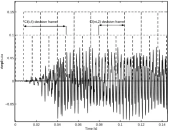
Segmentation of the whole sound database was per-formed with the two methods described in section 2. For fixed-length segmentation, two lengths were used: 2 windows (about 60 ms) and 4 windows (about 120 ms). Each segmentation is used to gen-erate two datasets: a transient-window dataset, and the complementary one, the non-transient-window dataset. On Figure 3, two examples of decision frames are shown: the Cl(t,4) decision frame, tak-ing 4 overlapptak-ing windows at the transient location, and the Cl(nt, 2) taking 2 overlapping windows in a non-transient part of the signal.
0 0.02 0.04 0.06 0.08 0.1 0.12 0.14 −0.05 0 0.05 0.1 0.15 Time [s] Amplitude
Cl(t,4) decision frame Cl(nt,2) decision frame
Fig. 3: Examples of decision frames, dashed-line rectangles represent overlapping analysis windows. 5.2. Efficiency of features selected over different segments
Pairwise feature selection was performed on the fol-lowing data sets to obtain the 40 most relevant ones (for each pair):
• 3 datasets including observations from segments labeled as transient (the related selected feature sets will be referred to as FS(t,2), FS(t,4) and FS(t,a)), where FS(t,2) (resp. FS(t,4)) is the se-lected feature set on the transient segments for segment of length 2 (resp. 4), and FS(t,a) the selected feature set on the frames with adaptive transient lengths).
• 3 datasets including observations from the remaining segments labeled as non-transient
Essid et al. transient/steady-state segments in instrument recognition
by the same segmentation methods (FS(nt,2), FS(nt,4) and FS(nt,a) sets, same notations as above);
• the “baseline” dataset including all observa-tions regardless of the transientness of the signal (FS(b)).
Significant variability is observed on the subsets of features selected for each pair of instruments over the considered datasets. FSA outputs have been posted on the web3 for interested readers to look
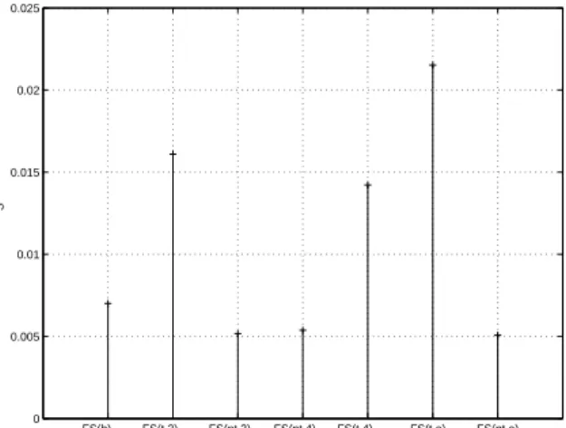
into it in depth. FS(b) FS(t,2) FS(nt,2) FS(nt,4) FS(t,4) FS(t,a) FS(nt,a) 0 0.005 0.01 0.015 0.02 0.025 S
Fig. 4: Mean class separability (over all class pairs) with features selected on different segments. Class separability measures (see section 3.2) result-ing from all previous feature sets are depicted in fig-ure 4 from which the following can be deduced:
• S values obtained with transient segment data (FS(t,2), FS(t,4), FS(ta)) are greater than values reached by non-transient (FS(nt,2), FS(nt,4), FS(nta)) and FS(b), hence a better class separability is achieved using descriptors specifically selected for the transient segment data (regardless of the segmentation method used);
• among the segmentation methods, the adaptive one (FS(t,a)) gives rise to observations which,
3
see www.tsi.enst.fr/˜essid/pub/pubAES118/
when processed with the adapted features, en-ables the best discrimination between instru-ments;
• data from the non-transient segments results in poor class separability, smaller than the one yielded by the undifferentiated processing (FS(b)).
These results thus confirm the widespread assertion that attack-transients are particularly relevant in in-strument timbre discrimination.
5.3. Classification over different segments
Based on the different sets of selected features (described in section 5.2) we proceed to SVM clas-sification of the musical instruments exploiting only the transient, only the steady-state or all the audio segments. Recognition success is evaluated over a number of decision frames. Each decision frame combines elementary decisions taken over Lt, Lnt or
L consecutive analysis windows respectively for the transient-based classifier, the non-transient-based classifier and the generic classifier (exploiting all audio segments).
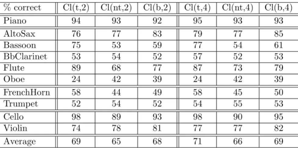
Table 2 sums up the the recognition accuracies found in the following situations:
• classification based on FS(t,Lt), FS(nt,Lnt) and
FS(b) with Lt= Lnt= L = 2;
• classification based on FS(t,Lt), FS(nt,Lnt) and
FS(b) with Lt= Lnt= L = 4.
The decision frame lengths were thus chosen in order to enable a fair comparison of the classifica-tion performance of the different schemes. Note that these lengths are imposed by the lengths of the transient segments which implies Lnt= Lt and
L= Lt.
On average better classification is achieved when using the transient segments, this is true for the two tested transient-segment lengths. Better results are found, on average, with Lt = 4. It can be said
that transients are essential for proper machine
AES 118th
Convention, Barcelona, Spain, 2005 May 28–31 Page 7 of 10
% correct Cl(t,2) Cl(nt,2) Cl(b,2) Cl(t,4) Cl(nt,4) Cl(b,4) Piano 94 93 92 95 93 93 AltoSax 76 77 83 79 77 85 Bassoon 75 53 59 77 54 61 BbClarinet 53 54 52 57 52 53 Flute 89 68 77 87 73 79 Oboe 24 42 39 24 42 39 FrenchHorn 58 44 49 58 45 50 Trumpet 52 54 52 54 55 53 Cello 98 89 93 98 90 95 Violin 74 78 81 77 77 82 Average 69 65 68 71 66 69
Table 2: Results of classification based on FS(t,Lt), FS(nt,Lt) and FS(b) with Lt= 2 and Lt= 4, respectively
Cl(t,2), Cl(nt,2), Cl(b,2), Cl(t,4), Cl(nt,4), Cl(b,4)
recognition of instruments as the worst results are obtained when they are not taken into consideration.
Nevertheless, looking at individual accuracies, one can note interesting exceptions. A glaring one is the oboe’s which is clearly better classified when the focus is put on its non-transient segments (42% on non-transients against 24% on transients). Since we consider that 1% differences are not statistically consistent, this is the only case where non-transient segments lead to better classification performance. It can be noted that the recognition accuracies of the alto sax and the violin found with the generic classifier are better compared to the transient-segment one. In fact, the undifferentiated processing leads to more successful classification in these cases. The confusion matrices reveal that the alto sax is more frequently confused with the violin when examined over the transient segments while the violin is more often classified as cello, Bb clarinet and alto sax (even though less confused with trumpet).
Table 3 shows the recognition accuracies of a “more realistic system”, where longer decision frames are tolerated, using a generic classifier. Better overall performance is achieved compared to a classifica-tion scheme exploiting only transient-segment deci-sion frames. It can be concluded that processing only the information of the transient windows is not
sufficient to improve the results of generic classifiers, when decision is taken in a fixed-length frame of re-alistic size. According to the high scores obtained on transient frames, developing a fusion system merging both transient and non-transient windows informa-tions contained in such a frame could be of interest.
% correct Cl(b,30) Cl(b,120) Piano 97 99 AltoSax 90 95 Bassoon 64 74 BbClarinet 57 62 Flute 84 89 Oboe 37 60 FrenchHorn 57 72 Trumpet 60 63 Cello 99 100 Violin 85 87 Average 73 80
Table 3: Classification results with L = 30 and L = 120
6. CONCLUSIONS
In this paper we studied the pertinence of using a differentiated transient/steady-state processing for automatic classification of musical instruments on solo performances. Transient windows tend to con-centrate relevant information for music instrument
Essid et al. transient/steady-state segments in instrument recognition
identification. In fact, it has been shown that, in most cases, transient-segment observations lead to a better instrument discrimination (regardless of the method used to perform the segmentation).
Nevertheless, in the perspective of developing a realistic machine recognition system wherein a fixed decision-frame length is imposed (typically 1 or 2s for realtime systems), it is not straightforward to optimally exploit such segmentations. Indeed, bet-ter classification performance can then be achieved when an undifferentiated processing is performed on all signal windows compared to the case where the decision is taken only on the transient-signal windows within the decision frame.
Systems adequately merging expert classifiers based on transient and steady-state segments should be de-signed to enable a better overall performance. Fur-thermore, to complete this study, specific transient parameters could be developed.
7. ACKNOWLEDGEMENTS
The authors wish to thank Marine Campedel for fruitful discussions on current feature selection tech-niques.
8. REFERENCES
[1] M. Clark, P. Robertson, and D. A. Luce. A preliminary experiment on the perceptual basis for musical instrument families. Journal of the Audio Engenieering Society, 12:199–203, 1964. [2] McAdams S., Winsberg S., de Soete G., and
Krimphoff J. Perceptual scaling of synthesized musical timbres: common dimensions, specfici-ties and latent subject classes. Psychological Research, (58):177–192, 1995.
[3] A. Eronen. Comparison of features for musi-cal instrument recognition. In Proceedings of WASPAA, 2001.
[4] J.P. Bello, C. Duxbury, M. Davies, and M.B. Sandler. On the use of phase and energy for musical onset detection in the complex domain. IEEE Signal Processing Letters, 2004.
[5] J.P. Bello, L. Daudet, S. Abdallah, C. Duxbury, M. Davies, and M.B. Sandler. A tutorial on on-set detection in music signals. IEEE Transac-tions on Speech and Audio Processing, 2005. to be published.
[6] P. Leveau, L. Daudet, and G. Richard. Method-ology and tools for the evaluation of automatic onset detection algorithms in music, submitted. Proceedings of ISMIR 2004, 2004.
[7] M. Goodwin and C. Avendano. Enhancement of audio signals using transient detection and modification. In Proceedings of the 117th AES Convention, 2004.
[8] Geoffroy Peeters. A large set of audio features for sound description (similarity and classifica-tion) in the cuidado project. Technical report, IRCAM, 2004.
[9] Judith C. Brown. Musical instrument identi-fication using autocorrelation coefficients. In International Symposium on Musical Acoustics, pages 291–295, 1998.
[10] Antti Eronen. Automatic musical instrument recognition. Master’s thesis, Tampere Univer-sity of Technology, April 2001.
[11] Lawrence R. Rabiner. Fundamentals of Speech Processing. Prentice Hall Signal Processing Se-ries. PTR Prentice-Hall, Inc., 1993.
[12] Olivier Gillet and Ga¨el Richard. Automatic transcription of drum loops. In IEEE Inter-national Conference on Acoustics, Speech and Signal Processing (ICASSP), Montral, Canada, May 2004.
[13] Slim Essid, Ga¨el Richard, and Bertrand David. Efficient musical instrument recognition on solo performance music using basic features. In AES 25th International Conference, London, UK, June 2004.
[14] Information technology - multimedia content description interface - part 4: Audio, jun 2001. ISO/IEC FDIS 15938-4:2001(E).
AES 118th
Convention, Barcelona, Spain, 2005 May 28–31 Page 9 of 10
[15] Judith C. Brown, Olivier Houix, and Stephen McAdams. Feature dependence in the auto-matic identification of musical woodwind in-struments. Journal of the Acoustical Society of America, 109:1064–1072, March 2000.
[16] Slim Essid, Ga¨el Richard, and Bertrand David. Musical instrument recognition based on class pairwise feature selection. In 5th Interna-tional Conference on Music Information Re-trieval (ISMIR), Barcelona, Spain, October 2004.
[17] Ron Kohavi and G. John. Wrappers for feature subset selection. Artificial Intelligence Journal, 97(1-2):273–324, 1997.
[18] A. L. Blum and P Langley. Selection of rele-vant features and examples in machine learning. Artificial Intelligence Journal, 97(1-2):245–271, December 1997.
[19] I. Guyon and A Elisseeff. An introduction to feature and variable selection. Journal of Ma-chine Learning Research, 3:1157–1182, 2003. [20] Geoffroy Peeters. Automatic classification of
large musical instrument databases using hier-archical classifiers with inertia ratio maximiza-tion. In 115th AES convention, New York, USA, October 2003.
[21] Slim Essid, Ga¨el Richard, and Bertrand David. Musical instrument recognition by pairwise classification strategies. IEEE Transactions on Speech and Audio Processing, 2004. to be pub-lished.
[22] Richard Duda and P. E. Hart. Pattern Clas-sification and Scence Analysis. Wiley- Inter-science. John Wiley & Sons, 1973.
[23] Vladimir Vapnik. The nature of statistical learning theory. Springer-Verlag, 1995.
[24] Christopher J.C. Burges. A tutorial on support vector machines for pattern recognition. Jour-nal of Data Mining and knowledge Discovery, 2(2):1–43, 1998.
[25] B. Sholkopf and A. J. Smola. Learning with kernels. The MIT Press, Cambridge, MA, 2002.
[26] John C. Platt. Probabilistic outputs for sup-port vector machines and comparisions to reg-ularized likelihood methods. 1999.