HAL Id: hal-02492258
https://hal.archives-ouvertes.fr/hal-02492258
Submitted on 26 Feb 2020
HAL is a multi-disciplinary open access
archive for the deposit and dissemination of
sci-entific research documents, whether they are
pub-lished or not. The documents may come from
teaching and research institutions in France or
abroad, or from public or private research centers.
L’archive ouverte pluridisciplinaire HAL, est
destinée au dépôt et à la diffusion de documents
scientifiques de niveau recherche, publiés ou non,
émanant des établissements d’enseignement et de
recherche français ou étrangers, des laboratoires
publics ou privés.
Matteo Acclavio, Roberto Maieli
To cite this version:
Matteo Acclavio, Roberto Maieli. Generalized connectives for multiplicative linear logic. CSL 2020
-28th EACSL annual conference on Computer Science Logic, Jan 2020, Barcelona, Spain. pp.6:1-6:15,
�10.4230/LIPIcs.CSL.2020.6�. �hal-02492258�
Logic
Matteo Acclavio
Samovar, UMR 5157 Télécom SudParis and CNRS, 9 rue Charles Fourier, 91011 Évry, France http://matteoacclavio.com/Math
Roberto Maieli
Mathematics & Physics Department, Roma Tre University, L.go S. L. Murialdo 1, 00146 Rome, Italy http://logica.uniroma3.it/maieli
Abstract
In this paper we investigate the notion of generalized connective for multiplicative linear logic. We introduce a notion of orthogonality for partitions of a finite set and we study the family of connectives which can be described by two orthogonal sets of partitions.
We prove that there is a special class of connectives that can never be decomposed by means of the multiplicative conjunction ⊗ and disjunction`, providing an infinite family of non-decomposable connectives, called Girard connectives. We show that each Girard connective can be naturally described by a type (a set of partitions equal to its double-orthogonal) and its orthogonal type. In addition, one of these two types is the union of the types associated to a family of MLL-formulas in disjunctive normal form, and these formulas only differ for the cyclic permutations of their atoms.
2012 ACM Subject Classification Theory of computation → Linear logic
Keywords and phrases Linear Logic, Partitions Sets, Proof Nets, Sequent Calculus
Digital Object Identifier 10.4230/LIPIcs.CSL.2020.6
1
Introduction
In his seminal paper [7], Girard introduced the notion of generalized multiplicative connective for linear logic [6] expressed in terms of permutations over finite sets. This work was then improved by Danos and Regnier in [5] where permutations were replaced by the weaker structure of partitions of finite sets. In particular, the original orthogonality condition for permutations proposed by Girard is replaced by the following:
two partitions on the same finite domain are orthogonal iff the (bipartite) multigraph with vertices the blocks of the two partitions and edges between blocks sharing an element
is connected and acyclic (ACC for short).
This orthogonality relation is extended to sets of partitions: two sets of partitions P and Q are orthogonal (denoted P ⊥ Q) if their elements are pairwise orthogonal (see Figure 1).
G1: [1, 2] [3] • • • [1, 2, 3] G2: [1, 2] [3] • • • • [1, 3] [2] G3: [1, 2] [3] • • • • [1] [2, 3]
Figure 1 The two partitions h[1, 2], [3]i and h[1, 2, 3]i are not orthogonal since G1contains a cycle.
The two sets of partitions P = {h[1, 2], [3]i} and Q = {h[1, 3], [2]i, h[1], [2, 3]i} are orthogonal.
© Matteo Acclavio and Roberto Maieli;
a1 a2 a3 ` ⊗ F test a1 a2 a3 • ◦ • F and a1 a2 a3 • ◦ • F P• F = {h[0, 2, 3], [1]i , h[0, 1, 3], [2]i} a⊥1 a ⊥ 2 a ⊥ 3 ⊗ ` F⊥ test a⊥1 a ⊥ 2 a ⊥ 3 • • ◦ F⊥ and a⊥1 a ⊥ 2 a ⊥ 3 • ◦ • F⊥ P• F⊥ = {h[0, 1, 2], [3]i , h[1, 2], [0, 3]i} Figure 2 The pretype of the formulas F = (a1` a2) ⊗ a3 and F⊥= (a⊥1 ⊗ a
⊥ 2)` a
⊥ 3.
Multiplicative linear logic has two well-known proof systems: sequent calculus and proof nets. Thus, we are able to associate sets of partitions to multiplicative formulas F = F (a1, . . . , an) by means these two syntaxes.
In the sequential syntax, a partition keeps the information about how the literals a1, . . . , an
occurring in F are gathered between its m premise sequents. In this way, we can see a (non-logical) derivation of F from a1, . . . , an as a generalized m-ary rule of the sequent calculus
and this rule is completely characterized by the organization of its premises – i.e. how premise atoms are split into sequents. This is possible because multiplicative rules are linear, that is conservative with respect to literals, and unconditional, that is context-free. By means of example, consider the following (non-logical) derivation of F (a1, a2, a3) = (a1` a2) ⊗ a3and
its associated generalized rule ρ: a1, a2 ` a1` a2 a3 ⊗ (a1` a2) ⊗ a3 ! aF (a1, a2 a3 ρ 1, a2, a3)
Then, the organization of F is the same of its unique associated generalized rule ρ, that is OF = {h[1, 2], [3]i} = Oρ. However, if we consider its dual formula F⊥(a⊥1, a⊥2, a⊥3) =
(a⊥1 ⊗a⊥2)`a⊥3 we observe two possible derivations associated to two possible generalized rules ρ1 and ρ2 and that OF⊥ = {h[1, 3], [2]i, h[2, 3], [1]i} = Oρ1∪ Oρ2 since Oρ1 = {h[1, 3], [2]i}
and Oρ2= {h[2, 3], [1]i}. Moreover OF ⊥ OF⊥.
a⊥ 1, a⊥3 a⊥2 ⊗ a⊥ 1 ⊗ a⊥2, a3 ` (a⊥ 1 ⊗ a⊥2)` a⊥3 ! a ⊥ 1, a⊥3 a⊥2 ρ 1 F⊥(a⊥1, a⊥2, a⊥3) a⊥ 2, a⊥3 a⊥1 ⊗ a⊥ 1 ⊗ a⊥2, a3 ` (a⊥ 1 ⊗ a⊥2)` a⊥3 ! a ⊥ 2, a⊥3 a⊥1 ρ 2 F⊥(a⊥1, a⊥2, a⊥3)
In the graphical syntax (i.e. proof structures), a partition keeps the information about how the premises are gathered by a Danos-Regnier switching [5] in the correction graph of the proof structure with premises a1, . . . , an and the conclusion of a MLL-formula F (i.e. the
formula tree of F ). However, as already observed in [12], this construction gives another key information: not all blocks of a partition have the same statute. In fact, only one of its block is principal, that is, it is connected with the conclusion. To keep this information, we consider the set of pointed partitions, i.e. partitions over {0, 1, . . . , n} where 0 is a marking for principal blocks of a formula F (a1, ..., an): we call this set, the pretype of F , denoted by
P•
F (see Figure 2). Once we define a forgetting function b−c erasing the occurrence of 0 in a
pointed partition, we observe that bPF•c ⊥ bP•
F⊥c.
The sequential and the graphical way to associate a set of partitions to a MLL-formula F (a1, . . . , an) are in some sense orthogonal since we can show that OF = bPF•c⊥.
This construction suggests a natural generalization for sequent calculus: given two sets of
partitions P and Q over {1, . . . , n} such that P ⊥ Q and Q = P⊥ (or P = Q⊥), we define
a pair of generalized multiplicative connectives C = C(P,Q) and C⊥ for which we assume
given a set of sequent rules. Each rule introducing C or C⊥ has as organization a partition
in P or respectively Q. Moreover, the orthogonality of P and Q assures the existence of a cut-elimination procedure.
Analogously, in proof structures syntax, given two sets of pointed partitions P• and
Q• over {0, 1, . . . , n} such that bP•c ⊥ bQ•c and bP•c⊥⊥ bQ•c⊥, we define a pair of dual
multiplicative connectives satisfying cut-elimination. The information given by the pointed partitions allows us to define the Danos-Regnier switches for these connectives, since it gives us not only the information on how to gather the incoming edges of a node into blocks, but also which one of them is connected with the outgoing edge. This gives an extension of the correctness criterion for proof structures containing such connectives. Furthermore, the orthogonality of bP•c⊥ and bQ•c⊥ is mandatory for cut-elimination.
One natural question arises about the decomposability by means of ` and ⊗:
given a pair of partitions (P, Q) describing a multiplicative connective C(P,Q), is it always possible to find a MLL-formula F such that OF = P and OF⊥= Q?
A preliminary negative answer to this question is given by the non-decompsable connective G4 defined in [7] in terms of permutations, and here reported as reformulated in [5]:
G4= C(P,Q) with P = {h[1, 2], [3, 4]i, h[2, 3], [4, 1]i} and Q = {h[1, 3], [2], [4]i, h[2, 4], [1], [3]i}
In [11] the second author defines an infinite family of non-decomposable connectives generaliz-ing G4. Each (sequential) connective of this family is given by a set of two partitions P , called entangled pair1, together with its orthogonal set of partitions P⊥= {q | q ⊥ p for all p ∈ P }.
In this paper we make a step further with respect to [11] by providing an infinite class of sets of partitions Shu,vienabling us to define an infinite class of non-decomposable connectives
strictly including the entangled ones. We show that this set of partitions can be expressed as the union of the types of a family of formulas obtained by all the possible cyclic permutations of the literals of a formula F (a1, . . . , an) = (a1,1⊗ · · · ⊗ a1,n1)` · · · ` (ak,1⊗ · · · ⊗ ak,nk), i.e.
a MLL disjunctive normal form. Besides the combinatorial nature of this property, this allows to prove that if Shu,vi⊂ P , then any generalized connective C(P,Q) cannot be decomposable.
Non-decomposable connectives represent a new challenging research subject in linear logic: a denotational semantics and the geometry of interaction for the extension of MLL with these connectives are still missing. Moreover, we foresee an extension of Andreoli’s paradigm of modular proof construction, using such connectives as additional modules [3, 10].
Structure of the paper. In Section 2 we give some backgrounds on graphs and partitions of finite sets. In particular, we provide a family of partitions satisfying a property of closure with respect to a notion of orthogonality. Furthermore we recall some multiplicative linear logic definitions and results in Section 3. In Section 4 we explain the correspondence between partitions sets and generalized multiplicative connectives and in Section 5 we redefine the notions of decomposable connectives in graphical and sequential syntax. Finally in Section 6 we give the family of non-decomposable connectives called Girard connectives.
1 A pair of partitions, p and q, is entangled iff p and q have the same number of blocks and each block
2
Graphs and Partitions
A (direct) multigraph G = (V, E) is given by a set of vertices V and a multiset of edges E = {(u, v)|u, v ∈ V }. We denote u_v iff there is a (u, v) ∈ E and u6_v iff there is no (u, v) in E. A multigraph is undirected if the set of edges is reflexive, i.e. (u, v) ∈ E iff (v, u) ∈ E. Let u, v ∈ V , then a path form u to v is a sequence of vertices v0, . . . , vn ∈ V such that
vi_vi+1 for all i ∈ 0, . . . , n − 1.A multigraph is connected if for all u, v ∈ V there is a path
from u to v. A connected component of a graph is a maximal subset of connected vertices V0 ⊂ V . A path is a cycle if v
0= vn. A cycle is primitive if vi6_vj for all j 6= i + 1 with
i 6= 0 and j 6= n. A multigraph is acyclic if it contains no cycles. A graph is a multigraph such that E is a set of edges, i.e. there is at most one edge (u, v) for each pair of vertices u, v ∈ V .
ITheorem 1 (Euler-Poincaré invariance). Let G = (V, E) be a multigraph. If |Cy| and |CC| are respectively the number of primitive cycles and the number of connected components of G, then |V | − |E| + |Cy| − |CC| = 0.
A partition p = hγ1, . . . , γui of a finite set X = {1, ..., n} is a set of subsets of X (an
element ofP(X)) such that X = Siγi and if i 6= j then γi∩ γj = ∅. We denote by PX
the set of partitions of a finite set X and Pn= P{1,...,n}. We call X the support of p and γi
a block of p. To simplify reading, we differentiate parenthesis for partitions and blocks as follows p = h[a1,1, . . . , a1,k1], . . . , [au,1, . . . , au,ku]i.
IDefinition 2 (Orthogonality). Let p, q ∈ Pn. The (undirected) graph of incidence of p and
q, denoted G(p, q), is the multigraph with vertices the blocks of p and q such that there is an edge vγ1_vγ2 for each element in γ1∩ γ26= ∅. We say that p and q are orthogonal, denoted
p ⊥ q, iff the induced multigraph G(p, q) is connected and acyclic (ACC for short).
The notion of orthogonality extends to set of partitions: if P, Q ⊂ Pn, we say that P and
Q are orthogonal (P ⊥ Q) iff they are pointwise orthogonal, that is p ⊥ q for all p ∈ P and q ∈ Q. If P ⊂ Pn, we denote P⊥= {q ∈ Pn| p ⊥ q for all p ∈ P } the orthogonal of P . For
an example refer to Figure 1.
From Theorem 1 we deduce the following
ICorollary 3. If p, q ∈ P ∈ Pn and |p| 6= |q| then P⊥ = ∅.
IDefinition 4 (Type). A set of partitions P ⊂ Pn is a type iff P = P⊥⊥.
We here recall some results form [12] which are useful to compute the orthogonal of a set of partitions and to decide whenever a set of partitions is a type.
IProposition 5 (Partitions and Orthogonality). Let A, B ⊂ Pn, then the following facts hold:
1. A⊥= A⊥⊥⊥. This means that A⊥ is a type;
2. A ⊥ B iff A ⊆ B⊥ and A ⊥ B iff B ⊆ A⊥;
3. A ⊆ B implies B⊥⊆ A⊥;
4. if A is a type, then there is B such that A = B⊥;
5. (S iAi) ⊥=T iA ⊥ i ; 6. (T iAi)⊥⊇SiA⊥i ;
7. if A admits a set B such that A ⊥ B then all partitions in A have the same cardinality. In particular, the intersection of types is always a type, while the union is not.
h[1, 2], [3, 4], [5, 6]i h[2, 3], [4, 5], [6, 1]i h[1, 2, 3], [4, 5, 6], [7, 8, 9]i h[2, 3, 4], [5, 6, 7], [8, 9, 1]i h[3, 4, 5], [6, 7, 8], [9, 1, 2]i 1 2 3 4 5 6 1 2 3 4 5 6 1 2 3 4 5 6 7 8 9 1 2 3 4 5 6 7 8 9 1 2 3 4 5 6 7 8 9
Figure 3 Examples of basic partitions and their corresponding subdivision of the cycle in n parts.
IExample 6. Let P, Q ⊂ P4 be defined as
P = {p1= h[1, 3], [2, 4]i, p2= h[1, 4], [2, 3]i} and Q = {q1= h[1, 3, 4], [2]i, q2= h[2, 3, 4], [1]i
Then P⊥ = {p1}⊥∩ {p2}⊥ = {h[3, 4], [1], [2]i, h[1, 2], [3], [4]i} and Q⊥ = {q1}⊥∩ {q2}⊥ =
{h[1, 2], [3], [4]i}. That is P is a type and Q is not.
ITheorem 7 (No sub-type). If T ⊂ Pn is a type, then there is no type T0 6= T such that
T0⊂ Pn and T0 ⊂ T .
Proof. By Proposition 5.3 if P ⊂ T then T⊥⊆ P⊥. In particular, T ⊥ P⊥. By Proposition
5.2 we have P ⊆ T⊥⊥. J
IDefinition 8 (Entangled pairs of partitions [11]). A pair of partitions P = {p, q} ⊂ Pn with
p 6= q is an entangled pair if |p| = |q| and 1 ≤ |γ| ≤ 2 for each γ ∈ p ∪ q.
By means of example, the set P and P⊥ given in Example 6 are both entangled pairs.
ITheorem 9 (Entangled types [11]). Every entangled pair of partitions P ⊂ Pn is a type.
2.1
Basic Partitions
For the rest of this paper we assume n ∈ N such that n = uv for some u, v > 1.
A basic partition of n is a partition p ∈ Pn with u blocks of v elements such that each
block is of the form [i, i + 1, . . . , i + v − 1], if i + v − 1 ≤ n, or [i, . . . , n, 1, 2, . . . , i + v − 1 − n] otherwise. Intuitively, if we place the elements in {1, . . . , n} over a circle in an increasing order, a basic partition can be viewed as a subdivision of that circle into u intervals containing v elements as shown in Figure 3.
IDefinition 10 (Space of basic partitions). We call the space of basic partitions of rank hu, vi, denoted Shu,vi, the set of all possible basic partitions of n made of u blocks of v elements. That is, Shu,vi⊂ Pn is the following set
p1: h[1, . . . , v], [v + 1, . . . , 2v], . . . , [v(u − 1) + 1, . . . , n]i p2: h[2, . . . , v + 1], [v + 2, . . . , 2v + 1], . . . , [v(u − 1) + 2, . . . , n, 1]i . . . ...
pi: h[i, . . . , v + (i − 1)], [v + i, . . . , 2v + (i − 1)], . . . , [v(u − 1) + i, . . . , n, 1, . . . , i − 1]i . . . ... pv: h[v, . . . , 2v − 1], [2v, . . . , 3v − 1], . . . , [n, 1, . . . , v − 1]i
Some examples of spaces with different rank are given in Figure 4.
ILemma 11 (Cardinality of Shu,vi). If Shu,vi is a space of rank hu, vi, then |Shu,vi| = v.
Sh3,2i= {h[1, 2], [3, 4], [5, 6]i, h[2, 3], [4, 5], [6, 1]i}
Sh2,3i= {h[1, 2, 3], [4, 5, 6]i, h[2, 3, 4], [5, 6, 1]i, h[3, 4, 5], [6, 1, 2]i}
Sh3,3i= {h[1, 2, 3], [4, 5, 6], [7, 8, 9]i, h[2, 3, 4], [5, 6, 7], [8, 9, 1]i, h[3, 4, 5], [6, 7, 8], [9, 1, 2]i}
Figure 4 Some examples of spaces of rank hu, vi.
q : h [i, v + i, . . . , (u − 1)v + i] , [b1] , . . . , [bu−1] , . . . , [bk(u−1)+1] , . . . , [b(k+1)(u−1)] , . . . , [bn−2u+1] , . . . , [bn−u] i
• • . . . • . . . • . . . • . . . • . . . •
• • •
p : h γ1 , γ2 , . . . , γu i
Figure 5 If p ∈ Shu,viand bi∈ {1, . . . , n} \ {i, v + 1, . . . , (u − 1)v + i} then p ⊥ q for q, p ∈ Pn.
IDefinition 12 (Distance). Given 1 ≤ i, j ≤ n, we define the distance of i and j modulo n δn(i, j) =
(
min{j − i, i − j + n} if j ≥ i
min{i − j, j − i + n} if j < i (1)
E.g the distance of 1 and 9 modulo n = 9 is 1 that is, δ9(1, 9) = min{8, 1}. ILemma 13 (Distance). Let 1 ≤ i, j ≤ n = uv.
δn(i, j) < v iff there is p ∈ Shu,vi containing a block γ such that i, j ∈ γ; δn(i, j) ≥ v iff for all p ∈ Shu,vi there are γ16= γ2∈ p such that i ∈ γ1, j ∈ γ2.
Proof. Since δn(i, j) = δn(j, i), we assume without losing generality that i < j. Hence, it
suffices to remark that Shu,vialways contains a partition including block [i, . . . , i + v − 1] if i + v − 1 ≤ n, or including block [i, i + 1, . . . , n, 1, 2, . . . , i + v − 1 − n] if i + v − 1 > n;
By similar reasoning. J
ILemma 14. If Shu,viis a space of basic partitions then its orthogonal S⊥hu,viis not empty.
Proof. Let q be the partition consisting of n − u + 1 blocks including a block [i = a1, . . . , au]
such that δn(ai, aj) = hv with h ∈ N for 1 < j ≤ u (called ith-block of congruence modulo v),
and n − u singleton blocks over {1, . . . , n} \ {a1, . . . , au}.
After Lemma 13 the multigraph G(p, q) is acyclic, that is |Cy| = 0. Hence, by Theorem 1,
p ⊥ q for all p ∈ Shu,vi(see Figure 5 for an intuition). J
ICorollary 15. All partitions of S⊥hu,vi have size 1 + n − u = 1 + u(v − 1).
Proof. It follows Lemma 14. J
Moreover, by simple arithmetic argument we have the following results:
ILemma 16. If p ∈ Shu,viand 1 ≤ i, j ≤ n = uv with δn(i, j) > v, then there is 1 ≤ k ≤ n
such that δn(i, j) = hv for a h ∈ N and δn(j, k) < v. That is, for each i, j there is a k at
distance a multiple of v from i which belongs to the same block of j in the partition p.
IProposition 17. If Shu,vi is a space of rank hu, vi, then:
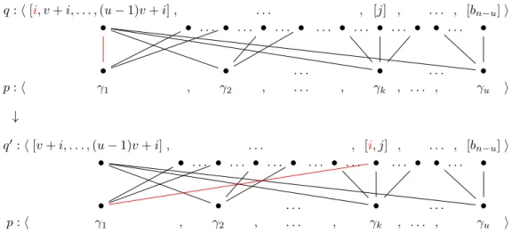
q : h [i, v + i, . . . , (u − 1)v + i] , . . . , [j] , . . . , [bn−u] i • • . . . • . . . • . . . • . . . • . . . • . . . • • . . . • • • . . . • . . . • p : h γ1 , γ2 , . . . , γk , . . . , γu i ↓ q0: h [v + i, . . . , (u − 1)v + i] , . . . , [i, j] , . . . , [bn−u] i • • . . . • . . . • . . . • . . . • . . . • . . . • • . . . • • • . . . • . . . • p : h γ1 , γ2 , . . . , γk , . . . , γu i
Figure 6 The permutation q including the ith-block of congruence modulo v and q0 are both ortogonal to p ∈ Shu,vi.
2. if 1 ≤ i, j ≤ n such that δn(i, j) ≥ v, then there is a partition q ∈ S⊥hu,vi containing a
block γ such that i, j ∈ γ.
Proof. 1. By Lemma 14, given 1 ≤ i, j ≤ n such that δ(i, j) > v and δ(i, j) = hv for h ∈ N,
there is a partition q containing the jth-block of congruence modulo v and all singleton
blocks is in S⊥
hu,vi. Hence, in q there is the singleton block [i].
2. if δn(i, j) = hv for a h ∈ N, then we consider the partition q made of the ith-block of
congruence modulo v and singleton blocks.
If δn(i, j) > v and δn(i, j) = hv for a h ∈ N we define a partition q0 from q by removing i
form the ith-block of congruence modulo v and adding i to the singleton [j] as shown
in Figure 6. To prove that q0 ∈ S⊥
hu,vi it suffices to use Lemma 16. In fact, we can
assume that i belongs to γi ∈ p ∈ Shu,vi. Then there is k such that i ∈ γk for any
p ∈ Shu,vi. Since j 6= i + hv with h ∈ N, then γk6= γ1. By Theorem 1, G(q0, p) is acyclic
and connected, hence q0⊥ p. J
ITheorem 18. Every space of basic partitions Shu,vi is a type.
Proof. Assume by contradiction that Shu,vi is not a type, i.e. assume there exists p0 ∈
(S⊥hu,vi)⊥ such that p0 ∈ S/ hu,vi. By Proposition 17.1, p0 cannot contain any singleton block
[i]. Moreover, by Proposition 17.2, p0 cannot contain any block γ such that i, j ∈ γ and
δn(i, j) ≥ v. This means that p0 consists only of blocks containing elements at distance
strictly smaller than v, hence |p0| > u. This contradicts Proposition 5.7. J
3
Multiplicative Linear Logic Backgrounds
We consider the class F of multiplicative linar logic formulas (denoted by A, B, . . . ) in negation normal form, generated by a countable set A = {a, b, . . . } of propositional variables
by the grammar A, B ::= a | A⊥| A` B | A ⊗ B modulo the involution of (·)⊥ and the de
Morgan laws: A⊥⊥= A, (A ⊗ B)⊥= A⊥` B⊥ and (A` B)⊥= A⊥⊗ B⊥. A sequent is a
set of occurrences of formulas. If a ∈ A, we say that a and a⊥ are atoms or atomic formulas.
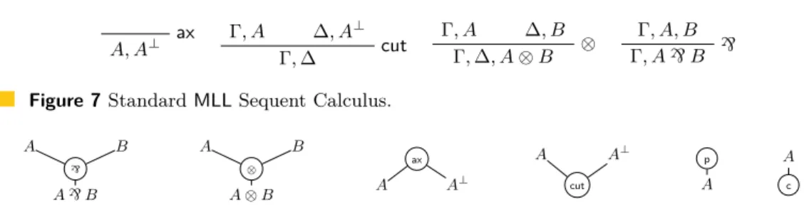
The sequent system for MLL is given by the rules in Figure 7. If ρ is a sequent system rule, we call active a formula in a premise of a rule which is not in its conclusion and and principal the formula introduced by the rule in the conclusion.
ax A, A⊥ Γ, A ∆, A ⊥ cut Γ, ∆ Γ, A ∆, B ⊗ Γ, ∆, A ⊗ B Γ, A, B ` Γ, A` B
Figure 7 Standard MLL Sequent Calculus.
A B ` A` B A B ⊗ A ⊗ B ax A A⊥ A A⊥ cut p A A c
Figure 8 Labels conditions for vertices and edges of a proof structures (also known as links).
IDefinition 19 (Proof Structure). A proof structure P is a direct graph with edges labeled by MLL-formulas and vertices labeled by {ax, cut, ⊗,`, p, c} according to conditions of Figure 8. We call premises ( conclusions) of a proof structure the nodes labeled by p (c). Moreover, abusing notation, we identify these nodes with the formula labeling the outgoing (respectively incoming) edge of these nodes. Similarly, we call premises ( conclusion) of a node its incoming (outgoing) edges labels.
To each derivation d with conclusion Γ in MLL we associate the proof structure Pd with
conclusions Γ defined as follows:
for all inference rule ρ in d there is a corresponding node in Pd labeled by ρ having as
premises the active formulas of ρ and as conclusion the principal formula of ρ; for each formula in the conclusion of d there is a node in Pd labeled by c.
IDefinition 20. A proof structure π is a proof net if there is a derivation d in MLL such that π = Pd.
We characterize proof nets by means of correctness conditions on proof structures.
I Definition 21 (Switching). A switching σ of a MLL proof structure P is a function associating to each `-node in P a switch, i.e. a block of the partition h[1], [2]i. For each switching, we define σ(P) as the undirected correction graph (also called test) obtained by forgetting the orientation of edges and by removing, for each`-node with conclusion A ` B, the edge labeled by B if its switch is [1] or the edge labeled by A if the switch is [2].
ITheorem 22 (Danos-Regnier sequentialization [5]). For each switching σ of π, the graph σ(π) is ACC iff there is a derivation d such that P = Pd.
The interest of proof nets lies on the fact that they allow of identify derivations which are equivalent modulo rules permutations. This simplifies the proof of cut-elimination theorem for MLL by eliminating the bureaucracy of rules permutations during cut-elimination procedure. The rewriting rules for proof structures cut-elimination are given in Figure 9.
I Theorem 23 (Danos-Regnier cut-elimination [5]). Cut-elimination procedure for proof structures is convergent and preserves connectedness and acyclicity.
4
Generalized multiplicative connectives and partitions sets
An n-ary connective is a syntactic symbol C we use to construct a new formula C(A1, . . . , An)
from the formulas A1, . . . , An in a formal grammar. By means of example, in MLL we have
only the (binary) connectives` and ⊗. We remark that in a complete sequent calculus,
each n-ary connective C admits at least one rule ρ with k ≤ n premise sequents with active formulas A1, . . . , An and principal formula C(A1, . . . , An).
A B A⊥ B⊥ ` ⊗ cut → A B A⊥ B⊥ cut cut A ax cut A → A A
Figure 9 Proof nets cut-elimination rewriting rules.
` Γ1, Ai1, . . . , Aik . . . ` Γm, Aih, . . . , Ain ρ C
` Γ1, . . . , Γm, C(A1, . . . , An)
Oρ= h[i1, . . . , ik], . . . , [ih, . . . in]i
Figure 10 A sequential rule ρ introducing the connective C and its associate partitionOρ.
conservative with respect of the atoms (or linear ), i.e. the premises of the rule have exactly the same atoms as the conclusion;
unconditional, i.e. the rule does not require information about the contexts.
As remarked in [7] and [5], these conditions allow us to associate set of partitions to multiplicative connectives of linear logic. In fact, in sequent calculus we can associate to each connective C the set of partitions describing how all the sequential rules introducing C gather the principal subformula between its premise sequents.
Similarly, by the Danos-Regnier correctness criterion, each switching of a MLL proof structure determines a partition corresponding to the premises belonging to the same connected component. However, some of the premises can never be connected to the root of a single-conclusion test of a proof net. For this reason, we prove in this paper that a set of partitions is not enough to describe a graphical connective, since each connective has to be given together with its possible switches. This additional information is provided by considering a special symbol to mark the principal block, i.e. the unique block selected by the switch to be connected to the conclusion.
4.1
Partitions and generalized sequential connectives
We can associate to a multiplicative rule (i.e. linear and context-free) of the sequent calculus
with n active formulas a partition in Pn. That is, a multiplicative m-ary rule ρC for a
generalized n-ary connective C is completely characterized by the organization of its principal subformulas A1, . . . , An (see Figure 10).
IDefinition 24 (Organization of a rule). Let ρ be an m-ary rule (i.e. a rule with m premise sequents) with n active formulas A1, . . . , An and principal formula C(A1, . . . , An). The
partition Oρ ∈ Pn associated to ρ is made of m blocks defined as follows: i, j belong to a
same block iff the formulas A1 and Aj belong to the same premise of ρ. We call Oρ the
organization of the rules ρ.
IExample 25. The organizations of the`-rule and the ⊗-rule are respectively {h[1, 2]i} and {h[1], [2]i}. Moreover, {h[1, 2]i} ⊥ {h[1], [2]i}.
This allows to describe an n-ary connective by means of a set of partitions.
IDefinition 26 (Generalized sequential connective). We says that a pair (P, Q) of non-empty sets of partitions in Pn is a description of (or it describes) a sequential n-ary connective if
P ⊥ Q and if Q = P⊥ or P = Q⊥.
If (P, Q) is a description of a n-ary sequential connective, we denote by C(P,Q)a sequential n-ary connective described by (P, Q) and by C⊥(P,Q)= C(Q,P) its dual connective – described by (Q, P ). We call O(C(P,Q)) = P the organization of C(P,Q).
The organization a sequential connective C = C(P,Q) can be interpreted as the set of the
organizations of the rules introducing C. That is, if C is a sequential connective described by (P, Q), we can think to O(C) as the organizations of some rules in a two-sided calculus introducing C in the right-hand side and the set O(C⊥) as the organizations of all the rules introducing C on the left-hand side (because O⊥C = OC⊥ is a type).
IRemark 27. If C(P,Q) is a generalized sequential connective, since Q 6= ∅, by Corollary 3
all its sequential rules have the same arity m = |p| for any p ∈ P .
Let C = {C1, . . . , Cn} be a set of multiplicative connectives, we define the generalized
C-multiplicative formulas FC extending F with the generalized connectives in C, that is, for all
C = C(P,Q)∈ C with P, Q ∈ Pn we extend the grammar of MLL-formulas with C(A1, . . . Ani)
and C⊥(A1, . . . Ani). Thus, for each p ∈ P , we define a sequential rule ρ
p
C introducing the
connective C(P,Q) such that Oρp
C = p (see Figure 10). We denote MLL(C) the extension of
MLL with the sequent rulesS
C∈C
S
p∈P{ρ p
C}.
ITheorem 28. The sequent system MLL(C) is cut-free, that is a sequent Γ in FC is derivable in MLL(C) ∪ {cut} iff it is in MLL(C).
Proof. The proof is given in [5]. It suffices to remark that the partitions sets describing C
and its dual C⊥describe the introduction rules for these connectives. Hence a cut-elimination step consist of replacing the cut-rule and the two rules ρ and ρ0 introducing the cut-formula
by cut-rules between the active formulas of ρ and ρ0. J
IExample 29. If we consider the partitions sets P = {h[1, 2], [3]i} and Q = {h[1, 2, 3]i},
we have P 6⊥ Q. If ρP and ρ0Q, are the corresponding sequent rules, we can not define a
cut-elimination step as shown below.
` Γ, A1, B2 ` ∆, C3 ρ ` Γ, ∆, ρ(A1, B2, C3) ` Γ, A1, B2, C3 ρ0 ` Γ, ρ0(A 1, B2, C3) ` Γ, A1, B2 ` ∆, C3 ρ ` Γ, ∆, ρ(A1, B2, C3) ` Σ, A1, B2, C3 ρ0 ` Σ, ρ0(A 1, B2, C3) cut ` Γ, ∆, Σ
4.2
Partitions and generalized graphical connectives
We associate to each correction graph of an MLL-proof structure with n premises and one single conclusion a partition in Pnwhere each block contains the indices of connected premises.
Hence, we are able to associate to each proof net a set of partitions corresponding to all its possible correction graphs where axiom nodes are replaced by pairs of premise nodes.
IDefinition 30 (Pointed partition). A pointed partition2 p• is defined as a partition of the set {0, k + 1, . . . , n} with k ∈ N such that [0] is not an allowed block of p•. We denote by P•n
the set of pointed partitions over the set {0, 1, . . . , n}. We define a forgetful map b−c : P{0,k+1,...,n}→ P{k+1,...,n}
which associates to each pointed partition p•a partition bp•c = p called underlying partition of p•given by removing the element 0 form its the non-singleton block in which occurs. Similarly if p• is a set of pointed partitions we denote by P = bp•c the set {p = bp•c | p•∈ p•}.
Intuitively, we use the element 0 to mark the principal block, i.e. the block containing the indices of the premises which are connected to the conclusion in a test.
With this definition, we define the analogous of Definition 26 for graphical connectives.
2 The name “pointed partition” is inspired by pointed spaces of topology, which are spaces where a specific
A 1 . . . An C C(A1, . . . , An) A 1 A2 A3 A4 A5 A6 C C(A1, . . . , An) p• A1 A2 A3 A4 A5 A6 • ◦ ◦ C(A1, . . . , An)
Figure 11 On the left: Labels conditions for generalized connectives. On the right: A node
labeled by the C(P•,Q•) with h[0, 1, 2, 4], [3, 5], [6]i = p•∈ P• and how this node is modified during
test computation when p•is its selected switch.
IDefinition 31 (Generalized Graphical Connectives). We say that the pair (P•, Q•) of non-empty sets of pointed partitions in P•n such that for all 0 < i ≤ n there is a block γ such that
{0, i} ⊂ γ ∈ p•∈ P• (respectively {0, i} ⊂ γ ∈ q•∈ Q•) is a description of (or it describes) a graphical n-ary connective if bP•c ⊥ bQ•c and if bP•c⊥⊥ bQ•c⊥.
We denote by C(P•,Q•) a graphical n-ary connective described by (P•, Q•) and by
C⊥(P•,Q•)= C(Q•,P•) its dual connective – described by (Q•, P•).
IExample 32. If P• = {h[1, 0], [2]i, h[1], [0, 2]i} and Q• = {h[0, 1, 2]i}, then` and ⊗ are respectively described by (P•, Q•) and (Q•, P•).
I Definition 33 (Generalized Proof Structure). Let C = {C(P•
1,Q•1), . . . , C(Pk•,Q
•
k)} be a set of graphical n-ary connectives. An MLL(C) proof structure is a direct graph P with edges labeled by MLL(C)-formulas and vertices labed by {ax, cut, ⊗,`, p, c} ∪ {C, C⊥}C∈C satisfying conditions in Figures 8 and 11.
As for MLL proof structure, in order to define a correctness criterion, we extend the notion of switching to graphical n-ary connectives.
IDefinition 34 (Switching). Let C be a set of generalized graphical connectives. A switching σ of a MLL(C) proof structure P is a function associating to each C(P•,Q•)-node (i.e. a node
labeled by C(P•,Q•)∈ C) a switch, i.e. a pointed partition p•∈ P•.
Each switching σ defines an undirected graph σ(P) (called correction graph or test) obtained by forgetting edge orientations and modifying each node v labeled by C(P•,Q•) with
switch p• ∈ P• as follows: for each block γ ∈ p• with 0 /∈ γ, disconnect the corresponding edges targeting v and we re-link them to a fresh target node vγ for each γ (see Figure 11).
IDefinition 35 (Pretype). Let F be a MLL(C) formula over the atoms a1, . . . , an and PF be
the unique proof structure with premise a1, . . . , an and conclusion F , i.e. PF is the formula
tree of F . For each switching σ of PF we define a pointed partition p•σ∈ P•n as follows:
i and j belong to the same block in p• iff ai and aj belongs to the same connected
component of σ(P);
i belongs in the same block 0 in p• iff a
i is connected to the conclusion of σ(P).
The pretype of F is the set PF• = {p•σ ∈ P•
n | σ is a switching of PF}. We call bPF•c the
Danos-Regnier pretype (or DR-pretype for short) of F . The type of F is the bi-orthogonal of DR-pretype, i.e. TF = bPF•c⊥⊥.
IDefinition 36 (Generalized Proof Net). A MLL(C)-proof structure P is a MLL(C)-proof net iff for each switching σ of P the graph σ(P) is ACC.
The computational meaning of generalized connectives is guaranteed by the fact that the elimination of a cut-vertex linking two vertices labeled by C and C⊥ preserves the correctness criterion [5]. This follows from Definition 31 of a graphical connective: the condition P ⊥ Q
is necessary for ACC of proof structures, while the condition P⊥ ⊥ Q⊥ is mandatory to
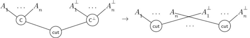
A 1 . . . An A ⊥ 1 . . . A ⊥ n C C⊥ cut → A1 . . . An A ⊥ 1 . . . A ⊥ n cut · · · cut
Figure 12 Generalized proof nets cut-elimination rewriting rule.
5
Decomposable connectives
In this section we study a notion of decomposability by means of ⊗ and` for generalized
connectives in both sequential and graphical sense. In particular, we provide a new definition of decomposability for graphical connectives which has to replace the one given in [5].
5.1
Sequential connectives
IDefinition 37 (Organization of a formula). If F = F (a1, . . . , an) is a MLL-formula, we
define the organization of F as the set of all partitions p ∈ Pn with p = hγ1, . . . , γki such that
there is a MLL-derivation of F form the premise sequents {ai}i∈γ1, . . . , {ai}i∈γk.
IDefinition 38 (Decomposable sequential connectives). A sequential connective C(P,Q) is
s-decomposable if there is a MLL-formula F such that P = OF (and Q = OF⊥).
I Example 39. Let P = {h[1, 3, 4], [2]i, h[2, 3, 4], [1]i, h[1, 3], [2, 4]i, h[1, 4], [2, 3]i} and Q = {h[1, 2], [3], [4]i}. Then C(P,Q)is s-decomposable. In fact P = OF for F = (a1⊗ a2)` a3` a4.
We show in Subsection 5.3 (Corollary 48) that if C is a s-decomposable sequential connective, then OC is a type.
5.2
Graphical connectives
As for the sequential case, we define a notion of decomposability for graphical connectives.
IDefinition 40 (Decomposable graphical connectives). A graphical n-ary connective C(P•,Q•)
is g-decomposable iff there is a MLL formula F (a1, . . . , an) such that P•= PF• and Q•= PF•⊥.
It is DR-decomposable if bP•c = bP•
Fc and bQ•c = bPF•⊥c.
ILemma 41. If a graphical connective is not DR-decomposable then it is not g-decomposable.
Proof. By absurd, let C(P•,Q•)be a g-decomposable graphical connective which is not
DR-decomposable. Thus, there is a MLL formula F such that P• = PF• and Q•= PF•⊥. Then
bP•c = bP•
Fc and bQ•c = bPF•⊥c. J
IExample 42. Let F = (((a1` a2) ⊗ a3) ⊗ a4)` a5 and P•
F = P
•
1 = {h[0, 1, 3, 4], [2], [5]i, h[1, 3, 4], [2], [0, 5]i, h[0, 2, 3, 4], [1], [5]i, h[2, 3, 4], [1], [0, 5]i}
PF•⊥ = Q
•
= {h[0, 1, 2, 5], [3], [4]i, h[0, 3, 5], [1, 2], [4]i, h[0, 4, 5], [1, 2], [3]i}.
Let P2• = P1•∪ {h[1, 3, 4], [0, 2], [5]i} and C1 = C(P•
1,Q•) and C2 = C(P2•,Q•). Then C1 and
C2 are both DR-decomposable, since bP1•c = bP2•c = bPF•c and bQ•c = bPF•⊥c, while
C1= C(P•
IProposition 43 (Switchings composition). Let F = F (a1, . . . , an) be a MLL-formula, then:
1. If F = F1(a1, . . . , ak)` F2(ak+1, . . . an) and σ is a switching of PF, there are p•1 ∈
P{0,1,...,m} and a p•2∈ P{0,m+1,...,n} pointed partitions associated respectively to a test of
PF1 and a test of PF2 such that p
•
σ∈ P•n is p•σ= bp•1c ∪ p•2 or p•σ = p•1∪ bp•2c.
2. If F = F1(a1, . . . , ak) ⊗ F2(ak+1, . . . an) and σ is a switching of PF, then there are
p•1 ∈ P{0,1,...,m} and a p•2 ∈ P{0,m+1,...,n} pointed partitions associated respectively to a test of PF1 and a test of PF2 such that p
•
σ∈ P•n is the pointed partition
p•σ = (p•1\ {γ1•}) ∪ (p2•\ {γ2•}) ∪ {γ1•∪ γ2•}
with γ1• and γ•2 respectively the blocks of p•1 and p•2 containing 0.
3. For all i ∈ {1, . . . , n} there is a p•∈ P•
F with γ ∈ p• such that {0, i} ⊂ γ.
Proof. 1. Since F = F1` F2, then every switching σ on PF is given by a switching σ1
on PF1, a switching σ2 on PF2 and a switch for the principal` node. If i, j > 0, then
i, j ∈ γ ∈ p•
σ iff their corresponding premise are connected in σ(PF). Thus i, j belong to
a same block iff there is a block in p•σ1 or in p•σ2 which contains both i and j.
For j = 0, since only one block may contain 0 accordingly with the switch of the principal `, i and 0 belong in the same block iff they are either in the same block in p•
σ1 or in p
•
σ2. 2. Similarly to the previous case. It suffices to remark that if i, j ∈ γ ∈ p•σ then either i and
j belong to the same block in p•σ1 or in p
•
σ2, or i and 0 belong to the same block in p
•
σ1
and j and 0 belong to the same block in p•σ2.
3. By induction over F . If F = a is an atomic formula then PF• = {h[1]i}, while if F = F1⊗F2
or F = F1` F2then i and 0 belong to the same block of a pointed partition in PF• iff i
and 0 belong to a same block of a partition in PF•
1∪ P
•
F2. J
IProposition 44 (Pretypes composition). Let F be a MLL-formula.
1. If F = F1` F2, then p• ∈ PF• iff p• = bp•1c ∪ p2• or p• = p•1∪ bp2•c with p•1 ∈ PF•1 and
p•2∈ PF•2.
2. If F = F1⊗ F2, then p•∈ PF• iff p•= (p•1\ {γ•1}) ∪ (p•2\ {γ2•}) ∪ {γ1•∪ γ2•} with p•1∈ PF•1
and 0 ∈ γ1•∈ p•1, and p•2∈ PF•2 and 0 ∈ γ
• 2 ∈ p•2.
Proof. It follows the constructions given in the proof of Proposition 44. J
ILemma 45. If F = F1` F2 is a MLL formula then |bPF•c| = |bPF•1c| · |bP
•
F2c|. Proof. Since bp•1∪ bp•
2cc = bbp•1c ∪ p•2c = bp•1c ∪ bp•2c, we conclude by Proposition 44. J
5.3
Correspondence between sequential and graphical connectives
There is a strong link between s-decomposable sequential and g-decomposable graphicalconnectives as exemplified by ⊗ and`:
b{h[0, 1, 2]i}c⊥ = {h[1, 2]i}⊥ = {h[1], [2]i} = O(⊗) b{h[1, 0], [2]i, h[1], [0, 2]i}c⊥
= {h[1], [2]i}⊥
= {h[1, 2]i} = O(`)
In fact, the two syntaxes are orthogonal views of a same decomposable connective:
IProposition 46 ([5]). If C(P•,Q•) is a g-decomposable graphical connective, then there is a
MLL formula F such that O(F ) = bPC•
(P • ,Q• )c
⊥.
IExample 47. If we consider the connective C given in the Example 39, bPP••c = bPF•c =
{h[1, 2], [3], [4]i, } with F = ((a1 ⊗ a2)` a3)` a4 and bPP••c⊥ = OF = {h[1, 3, 4], [2]i,
ICorollary 48. If C is a s-decomposable sequential connective, O(C) and O(C⊥) are types.
Proof. It is consequence of Propositions 5.4 and 46. J
6
Non-decomposable connectives
In this section we show that not all connectives are decomposable. We start by the following connective given in [7], then reformulated in [5]:
G4= C(P,Q) with P = {h[1, 2], [3, 4]i, h[2, 3], [4, 1]i} and Q = {h[1, 3], [2], [4]i, h[2, 4], [1], [3]i}
Following [11], G4 belongs to a class of non-decomposable connectives, called entangled, given
by two sets of partitions P and Q such that one of them is an entangled type (Definition 8).
We now define a more general class of non-decomposable connectives C(P,Q) where
P = Shu,viis a basic set of partitions. We then call such connectives Girard connectives. We
prove that these connectives are not decomposable and that whenever Shu,viis contained in
a set of partitions P then the connective C(P,Q) is non-decomposable (for any Q).
Moreover, if G is a Girard connective, the sequent G(a1, . . . , an), G⊥(a⊥1, . . . , a⊥n) admits
no η-exapaded proof in MLL(C) (this problem is known as “packaging problem”). In fact, since Girard connectives are not decomposable, this sequent is not stepwise derivable in MLL(C). In other words, for any C containing at least one non-decomposable connective, any sequent system for MLL(C) can not be an initial-coherent system [13].
I Definition 49 (Girard connectives). If Shu,vi is a space of basic partitions with u and v prime numbers, we call the sequential connective Chu,vi described by (Shu,vi, S⊥hu,vi) a
sequential Girard connective. Moreover, we call the graphical connective Chu,videscribed by (P•, Q•) a graphical Girard connective iff bP•c = Shu,vi and bQ•c = S⊥hu,vi.
ITheorem 50. Every Girard graphical connective is not DR-decomposable.
Proof. Let C(P•,Q•) be a Girard graphical connective. By definition this means that bP•c =
Shu,vi and bQ•c = S⊥hu,vi. By absurd, if C(P•,Q•) is DR-decomposable, then there is a
MLL-formula F such that bPF•c = Shu,vi and bPF•⊥c = S⊥hu,vi. Depending on F , we have
three cases:
if F is an atomic formula, then bPF•c = {h[1]i} 6= Shu,vi for any u, v ∈ N;
if F = F1` F2, by Lemma 45, v = |Shu,vi| = |bPF•c| = |bPF•1c| · |bP
•
F2c|. Since v is prime,
we can assume without loss of generality that bPF•
1c = {p1}, thus there is at least a block
γ ∈ p1 such that γ ∈ p for all p ∈ bPF•c;
if F (a1, . . . , an) = F1 ⊗ F2, we can assume without loss of generality that F1 = F1(a1, . . . , ak) and F2 = F2(ak+1,...,,an) with k + 1 > v. Thus, by Proposition 43.3,
there is a γ1∈ p•1∈ PF•1 such that 0, 1 ∈ γ1. Since k + 1 > v and n = uv, then there is
j ≥ k + 1 such that δn(i, j) ≤ v. Moreover, by Proposition 43.3, there is a γ2∈ p•2∈ PF•2
such that 0, j ∈ γ2. By Proposition 43.2 we conclude that there is γ ∈ p•∈ PF• such that
j, i ∈ γ, which is absurdum after Lemma 13. J
ICorollary 51. Every graphical Girard connective is not g-decomposable.
Proof. By Theorem 50 and Lemma 41. J
ICorollary 52. Every Girard connective is not s-decomposable.
ITheorem 53 (Danos-Regnier). Let P = bP•c and Q = bQ•c s.t. P = Q⊥ and Q = P⊥. Then a graphical connective C(P•,Q•) is DR-decomposable iff C(P,Q) is s-decomposable.
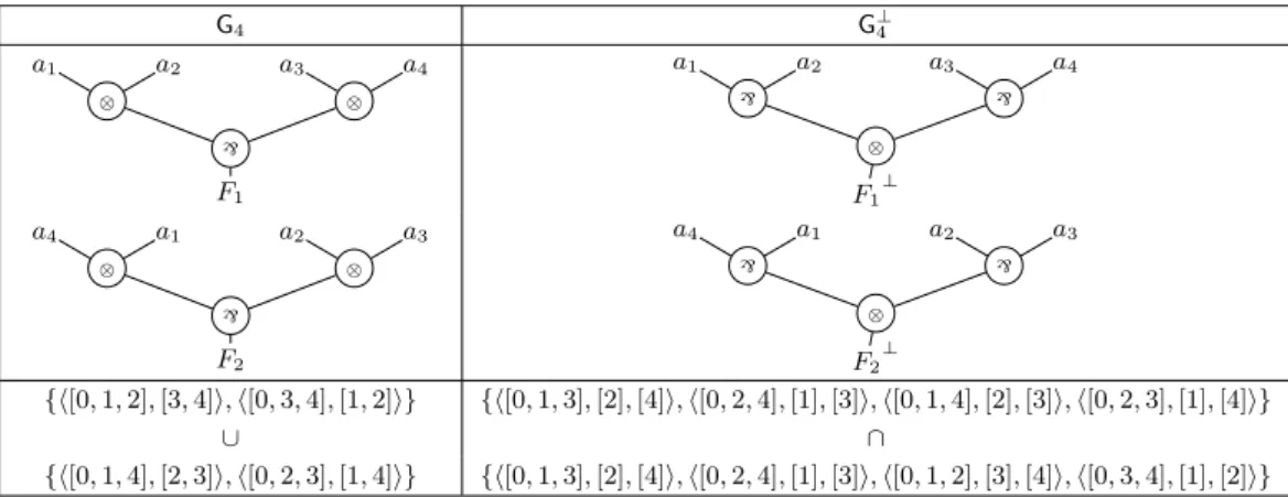
G4 G⊥4 a1 a2 a3 a4 ⊗ ⊗ ` F1 a1 a2 a3 a4 ` ` ⊗ F1 ⊥ a4 a1 a2 a3 ⊗ ⊗ ` F2 a4 a1 a2 a3 ` ` ⊗ F2 ⊥
{h[0, 1, 2], [3, 4]i, h[0, 3, 4], [1, 2]i} {h[0, 1, 3], [2], [4]i, h[0, 2, 4], [1], [3]i, h[0, 1, 4], [2], [3]i, h[0, 2, 3], [1], [4]i}
∪ ∩
{h[0, 1, 4], [2, 3]i, h[0, 2, 3], [1, 4]i} {h[0, 1, 3], [2], [4]i, h[0, 2, 4], [1], [3]i, h[0, 1, 2], [3], [4]i, h[0, 3, 4], [1], [2]i} Figure 13 The connectives G4= Ch2,2i and its dual connective G⊥4 seen respectively as the union
of DNF formulas pretypes and the intersection of CNF formula pretypes.
In [11] it is showed that P = Q⊥ and Q = P⊥ for every sequential connective C(P,Q).
ICorollary 54 (Completion of a sequential Girard connective). Let n = uv with u, v prime numbers, and P and Q non empty subsets of Pn. If C(P,Q) is a s-decomposable sequential, then Chu,vi6⊂ P and C⊥hu,vi6⊂ P .
Proof. By Theorem 18, both Shu,viand S⊥hu,viare types. Moreover, by Proposition 46, if
C(P,Q) is decomposable then P is a type. Then, by Theorem 7, none of Chu,viand C⊥hu,vican
be subsets of P . J
7
Conclusions and future works
In this paper we studied the generalized multiplicative connectives which can be described by two sets of pairwise orthogonal partitions. The orthogonality condition guarantees the definition of dual connectives for which cut-elimination is satisfied. Thus, multiplicative linear logic can be extended with these connectives preserving a computational interpretation.
We defined a notion of decomposability by means of ` and ⊗ for generalized connectives,
with respect to both sequent calculus and proof structures syntax. We then showed the existence of connectives which are not decomposable in both senses. In particular, we exhibited the existence of an infinite family of non-decomposable connectives called Girard connectives. For such non-decomposable generalized connectives, we gave an interpratation as superposition of special decomposable generalized connectives which are connectives associated to a family of MLL disjunctive normal forms.
The class of Girard connectives strictly includes the class of non-decomposable entagled connectives, thus extending the previous work of the second author on the same subject [11]. Although the definition of a Girard connective appears to be highly combinatorial, it admits the following simple geometrical interpretation. Every Girard connective in graphical syntax can be interpreted either as the union of the pretypes of a family of DNF formulas or as the intersection of the pretypes of a family of CNF formulas having the same formula tree but differing for the cyclic permutation of their atoms/leaves (see Figure 13). Observe that cyclic permutations can help to visualize the partition associated to those connectives (see Figure 3). This interpretation is not trivial since, by Proposition 5.6, the union of pretypes is not
necessarily a type. However, these connectives have no relation with the cyclic fragment of multiplicative linear logic [1]: neither the order among blocks nor the order among the elements of each block take role in the definition.
The existence of non-decomposable multiplicative connectives which do not admit any
sequentialization via the ⊗ and `, suggests future investigations on their geometry of
interaction [8], their connection to syntaxes for concurrency such as the π-calculus [14] and their denotational semantics [4] expanding the ideas given in [9] for syntectic connectives. Moreover, from the view point of logical programming with proof nets [3], non-decomposable graphical connectives provide additional modules. We foresee the use of the Girard connectives which may be interpreted as superposition of DNF for the definition of modules representing the superpositions of bipoles [2].
References
1 V. Michele Abrusci and Roberto Maieli. Proof nets for multiplicative cyclic linear logic and Lambek calculus. Mathematical Structures in Computer Science, 29(6):733–762, 2019. doi:10.1017/S0960129518000300.
2 Jean-Marc Andreoli. Focussing and proof construction. Annals of Pure and Applied Logic, 107(1):131–163, 2001. doi:10.1016/S0168-0072(00)00032-4.
3 Jean-Marc Andreoli and Laurent Mazaré. Concurrent construction of proof-nets. In
International Workshop on Computer Science Logic, pages 29–42. Springer, 2003. doi: 10.1007/978-3-540-45220-1_3.
4 Antonio Bucciarelli and Thomas Ehrhard. On phase semantics and denotational semantics in multiplicative–additive linear logic. Annals of Pure and Applied Logic, 102(3):247–282, 2000. doi:10.1016/S0168-0072(00)00056-7.
5 Vincent Danos and Laurent Regnier. The structure of multiplicatives. Archive for Mathematical
logic, 28(3):181–203, 1989. doi:10.1007/BF01622878.
6 Jean-Yves Girard. Linear logic. Theoretical Computer Science, 50(1):1–101, 1987. doi: 10.1016/0304-3975(87)90045-4.
7 Jean-Yves Girard. Multiplicatives. Rendiconti del Seminario Matematico, pages 11–34, 1987. 8 Jean-Yves Girard. On Geometry of Interaction. In Helmut Schwichtenberg, editor, Proof and
Computation, pages 145–191, Berlin, Heidelberg, 1995. Springer Berlin Heidelberg.
9 Jean-Yves Girard. On the meaning of logical rules II: multiplicatives and additives. NATO
ASI Series F Computer and Systems Sciences, 175:183–212, 2000.
10 Roberto Maieli. Construction of Retractile Proof Structures. In Gilles Dowek, editor, Rewriting
and Typed Lambda Calculi, pages 319–333. Springer International Publishing, 2014. doi:
10.1007/978-3-319-08918-8_22.
11 Roberto Maieli. Non decomposable connectives of linear logic. Annals of Pure and Applied
Logic, 170(11):102709, 2019. doi:10.1016/j.apal.2019.05.006.
12 Roberto Maieli and Quintijn Puite. Modularity of proof-nets. Archive for Mathematical Logic, 44(2):167–193, 2005. doi:10.1007/s00153-004-0242-2.
13 Dale Miller and Elaine Pimentel. A formal framework for specifying sequent calculus proof systems. Theoretical Computer Science, 474:98–116, 2013.
14 Robin Milner. Communicating and mobile systems: the Pi-calculus. Cambridge university press, 1999.
![Figure 1 The two partitions h[1, 2], [3]i and h[1, 2, 3]i are not orthogonal since G 1 contains a cycle.](https://thumb-eu.123doks.com/thumbv2/123doknet/12521425.341877/2.892.238.626.933.1027/figure-partitions-h-i-orthogonal-g-contains-cycle.webp)


![Figure 11 On the left: Labels conditions for generalized connectives. On the right: A node labeled by the C (P • ,Q • ) with h[0, 1, 2, 4], [3, 5], [6]i = p • ∈ P • and how this node is modified during test computation when p • is its selected switch.](https://thumb-eu.123doks.com/thumbv2/123doknet/12521425.341877/12.892.151.691.141.217/figure-labels-conditions-generalized-connectives-modified-computation-selected.webp)