HAL Id: hal-00725647
https://hal.archives-ouvertes.fr/hal-00725647
Submitted on 27 Aug 2012
HAL is a multi-disciplinary open access
archive for the deposit and dissemination of
sci-entific research documents, whether they are
pub-lished or not. The documents may come from
teaching and research institutions in France or
abroad, or from public or private research centers.
L’archive ouverte pluridisciplinaire HAL, est
destinée au dépôt et à la diffusion de documents
scientifiques de niveau recherche, publiés ou non,
émanant des établissements d’enseignement et de
recherche français ou étrangers, des laboratoires
publics ou privés.
A Practical Approach for 3D Model Indexing by
combining Local and Global Invariants
Jean-Philippe Vandeborre, Vincent Couillet, Mohamed Daoudi
To cite this version:
Jean-Philippe Vandeborre, Vincent Couillet, Mohamed Daoudi. A Practical Approach for 3D Model
Indexing by combining Local and Global Invariants. 1st IEEE International Symposium on 3D Data
Processing Visualization Transmission (3DPVT’02), Jun 2002, Padova, Italy. �hal-00725647�
A Practical Approach for 3D Model Indexing
by combining Local and Global Invariants
*Jean-Philippe Vandeborre, Vincent Couillet and Mohamed Daoudi
ENIC Telecom Lille I / INT (MIIRE group)
rue G.Marconi – cit´e scientifique - 59658 Villeneuve d’Ascq cedex – France
http://www-rech.telecom-lille1.enic.fr/MIIRE - email: vandeborre,daoudi
✁@enic.fr
*
this work has been partially supported by CNRS (Centre National de la Recherche Scientifique) France
Abstract
In this paper we present a three-dimensional model re-trieval system. In our approach, a three-dimensional model is described by three invariant descriptors: a curvature in-dex which consists of a histogram of the principal curva-tures of each face of the mesh, a histogram of distances between the faces, and a histogram of the volumes based on each face. This work focuses on extracting these invari-ant descriptors from the three-dimensional models, and on combining these descriptors in order to improve retrieval performance. An experimental evaluation demonstrates the satisfactory performance of our approach on a fifty three-dimensional models database.
1
Introduction
The use of three-dimensional image and model databases throughout the Internet is growing both in number and in size. The development of modeling tools, 3D scanners, 3D graphic accelerated hardware, Web3D and so on, is en-abling access to three-dimensional materials of high qual-ity. Techniques dealing with traditional information sys-tems have been adequate for many applications involving alphanumeric records. They can be ordered, indexed and searched for matching patterns in a straightforward manner. However, in many three-dimensional database applications, the information content of 3D models is not explicit, and is not easily suitable for direct indexing, classification and re-trieval. Different approaches exist to represent 3D models (VRML for instance). But the triangle mesh is the most widely used particularly because it is the format directly used by accelerated graphic hardware. A 3D model is de-scribed by a set of flat polygons – often triangles – which can be defined by listing their three-dimensional vertices and edges.
In this paper, we briefly describe three methods for com-puting three-dimensional shape signatures and dissimilarity measures. The first index is a curvature index, introduced by Koenderink [2]. The second one is a distance index intro-duced by Osada [3]. At last, the third index, introintro-duced by Zhang [7], is a volume index. Then, we propose to combine these three-dimensional shape signatures in different ways. The results obtained on a fifty three-dimensional models database show the effectiveness of our approach, and also the problems which are yet to be solved. We have used the classification matrices to look at the global performance of the single indices used individually, and the performance of our combining methods. At last, we present some conclu-sions and perspectives of our work.
2
Invariant descriptors
Indexing data is a way to find a suitable form for the in-formation, for a given application. This form is called an index. In a search engine, the role of the index is to repre-sent the original data in a very succinct manner. Intuitively, this means that the index should be invariant to some ge-ometric transformations of the object (translation, rotation, scaling), and should have a certain robustness to noise.
Three indices are used in our approach. The first one, curvature index [2], is a local index and is invariant to ge-ometric transformations, but it is not robust to noise. The second one, distance index [3], is a global index which is invariant to geometric transformations and is also robust to noise. Finally, volume index [7] is another local index which is invariant to geometric transformations and robust to noise, but not very discriminative as a stand-alone index.
2.1
Curvature index
The proposed three-dimensional curvature descriptor aims at providing an intrinsic shape description of
three-dimensional mesh models. It exploits some local attributes of the three-dimensional surface. The curvature index, in-troduced by [2], is defined as a function of the two principal curvatures of the surface. The main advantage of this index is that it gives the possibility to describe the shape of the object at a given point. The drawback is that it loses the information about the amplitude of the surface shape, and that it is also sensitive to noise.
Let✂ be a point on the three-dimensional surface. Let
us denote by✄✆☎
✝ and✄✟✞✝ the principal curvatures associated
with the point✂ . The curvature value at point✂ is defined
as: ✠ ✝☛✡ ✞☞✍✌✏✎✒✑✔✓✒✌✏✕✗✖✙✘ ✚✜✛ ✖✣✢ ✚ ✖ ✘ ✚✥✤ ✖ ✢ ✚✧✦✩★ ✓✒✪ ✄✆☎ ✝✬✫ ✄✭✞ ✝ . The curvature
index value belongs to the interval ✮✯✱✰✜✲✜✳ and is not defined
for planar surfaces. The curvature spectrum of the three-dimensional mesh is the histogram of the curvature values calculated over the entire mesh. The estimation of the prin-cipal curvatures is the key step of the curvature spectrum ex-traction. Computing these curvatures can be achieved in dif-ferent ways, each with advantages and drawbacks; [5] pro-poses five practical methods to compute them. We choose to compute the curvature at each face of the mesh by fitting a quadric to the neighborhood of this face (ie. the centroid of this face and the centroids of its 1-adjacent faces) using the least-square method. We can then calculate the princi-pal curvatures ✄✆☎ and ✄✭✞ as the eigenvalues of the
Wein-garten endomorphism✴
✡
✠
✤
☎✶✵✷✠✸✠ where✠ and✠✸✠ are
respectively the first and the second fundamental forms [1]. Hence, the curvature index can be computed with✠
✝ . We
now have✹✻✺✣✼✍✽✿✾✔❀❂❁ values, which can be represented as a
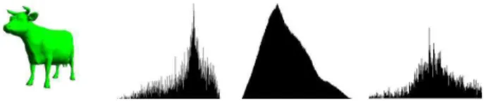
histogram. This histogram (1024 intervals) is our first index for the object. Figure 1 shows an example of a such spec-trum for the object quadru2 represented in the same figure.
2.2
Distance index
Global descriptors are a means to handle the object in its globality. This means that rather than being attached to the details of the object, we give more importance to its general aspect. In this case, the moments [4] are generally the tradi-tional mathematical tool. A new method has been recently proposed by [3], based on distance distributions. The main idea is to focus on the statistical distributions of a shape function measuring geometrical properties of the 3D model. They are represented as histograms, just as in the curvature index approach. The range of possible functions is very wide: from functions based on distances to functions based on angles. According to [3], the distance between random points gives good results compared to other methods. This index is globally robust to the noise but does not take the local deformation into account.
We take two random faces of the objects. Then we take two random points on those two faces. Finally, we com-pute the Euclidean distance between those two points. The
method is iterated✹ times,✹ being big enough to give an
accurate approximation of the distribution. We then build the histogram (1024 intervals) of all the values. Presently, the Euclidean distance, and thus this index, is not invariant by scaling. This is obviously because the Euclidean dis-tance is not invariant. So, we have to normalize the spec-trum before using it. One way is to normalize the mean value of the distribution. Figure 1 shows an example of a such distribution for the object quadru2 represented in the same figure.
2.3
Volume index
As a second local invariant, we have used the vol-ume distribution of a three-dimensional object based on [7]. The proposed method calculates the volume of three-dimensional objects as a mesh representation by computing the volume of each of the basic tetrahedrons composing the object. To compute each volume, we first have to be sure that all faces are triangular because we calculate the volume for tetrahedrons. The object is re-centered and so we calcu-late the volume of the tetrahedrons created with a triangu-lar face joined to the origin of the coordinate system:❃
✡ ☎❄✆❅❇❆✩❈✆❉✜❊ ✞✜❋✥☎❍● ❈ ✞ ❊✏❉ ❋✥☎❍● ❈✆❉✜❊ ☎✣❋■✞ ❆❏❈ ☎ ❊✏❉ ❋❍✞ ❆❏❈ ✞ ❊ ☎✔❋ ❉ ● ❈ ☎ ❊ ✞✙❋ ❉✙❑.
As done with the curvature index, a volume is computed for each face of the model. The results are then represented as a volume distribution histogram. This histogram is our second local index. Figure 1 shows an example of such a spectrum for the object quadru2 represented in the same fig-ure.
Figure 1. From left to right: object quadu2 (5804 faces), curvature, distance and volume histograms for this object
3
Comparing the histograms
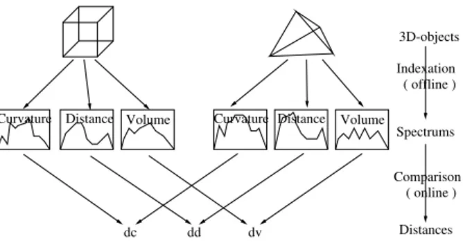
Each object is now described by three histograms which are used to compute a similarity between the objects, as shown in figure 2.
There are several ways to compare distribution spec-trum: the Minkowski Ln norms, Kolmogorov-Smirnov dis-tance, Match distances, and many others. We choose to use the L1 norm because of its simplicity and its accurate re-sults: ▲✏▼ ☎ ❅❖◆ ✲✏✰ ◆◗P✸❑ ✡❙❘❯❚ ✤ ❚❲❱ ◆ ✲ ❅❳❈❨❑❩❆❬◆◗P✟❅❳❈❨❑ ❱ ✵❂▲ ❈ . We
inter-polate the histograms in 64 linear segments by the least-square method in order to circumvent some problems like
3D-objects Spectrums Distances ( online ) Comparison ( offline ) Indexation
Distance Volume Distance Volume
dd dv Curvature Curvature
dc
Figure 2. Working scheme
quantization, noise etc. Then, a simple integration of these interpolations is made, giving a real number as a result. No-tice that although the same method is applied to the three types of histogram, the numbers given are not comparable.
4
Combining the results
We must now combine these different values described in the above section into one final mark. From now, please notice that the main goal of our approach is not to give an absolute distance between two objects, but rather to com-pare one object to many others in a database, specifically hunting for the nearest object to the request. Our results can then be relative to our database. We first compute the rank of each object according to each index, sorting them by decreasing values. We now have three integers, between 1 and❭❫❪✔❴✍❪❛❵✷❜■❝✣❞❇❡ , named❢❤❣✸✐❦❥✿❧ for the curvature index, ❢✶❣✷✐❦❥✷♠ for the distance index, and❢❤❣✷✐❦❥✷♥ for the volume
index. Those values are merged into a single one, using a formula. Intuitively, there are different strategies to merge these values:
♦
support the objects having satisfactory results with one approach, the other one having less importance. This is what we call the “OR” method:
♣❲qsr✏t✧✉✩✈❢✶❣✷✐❦❥✷✇ t①r■②❩③ ✈❢❤❣✷✐❦❥✷♠ t④r❍②⑤③ ✈❢❤❣✸✐❦❥✸♥ t①r■② ❭✻❪✜❴✍❪❛❵✷❜❍❝✔❞❇❡✍⑥⑦❭✻❪✔❴✍❪❛❵✷❜■❝✣❞❇❡❤⑥⑦❭✻❪✔❴✍❪❛❵✷❜■❝✣❞❇❡⑨⑧ ♦
use the mean of the three results. The “MEAN” method: ♣sq ✈ ❢✶❣✷✐❦❥✷✇❯⑩❶❢❤❣✷✐❦❥✸♠❷⑩❶❢❤❣✷✐❦❥✸♥ ② ❸ ③ ❭✻❪✜❴✍❪❛❵✷❜❍❝✔❞❇❡
This way, we now have one final real number, between 0 and 1, which represents the confidence one could have in the result. Note that the same kind of formula can be used to merge only two rank values. We have tested other methods of mixing rank values, but the two methods presented in this paper have given the best results.
5
Experiments and results
One of the biggest problems relating to search engines is their evaluation. As our database is classified (see section 5.1), we assume, for each request, that the objects from the same class as the request are relevant, and consequently the others are not. To evaluate the global performances of the different stand-alone indices and of our combining meth-ods, we have used classification matrices.
5.1
Three-dimensional models database
The methods described above have been implemented and tested on a 3D model database containing fifty mod-els which have been collected from the MPEG-7 3D shape core experiments [6] and arranged by ourselves into seven classes. Note that this manual classification has only been done for the purposes of our experiment. This classifi-cation is never used to improve the retrieval task of the search engine. The classes are the following: A-class (8 “airplanes” objects), M-class1 (5 “misc” objects), P-class
(7 “chess pieces” objects), H-class (8 “humans” objects), F-class (6 “fishes” objects), Q-class (8 “quadrupedes” ob-jects) and C-class (8 “cars” obob-jects). The models are simple meshes of approximatively 500 to 25000 faces, without any hierarchical structure. Moreover, it is important to notice that the mesh level of detail are very different from an ob-ject to another.
5.2
Classification matrix
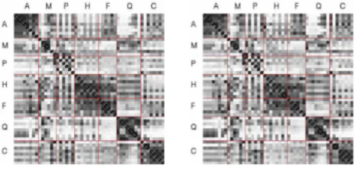
Each column of a classification matrix (eg. figure 3) rep-resents an object of the database (column 1 corresponds to object 1, etc.) which has been used as a request for the search engine. Each small square shows how the object of the given row was ranked. The darker the square is, the bet-ter the rank. For example the object number 23 was ranked last when the object 50 was requested, then the square at the intersection of column 50 and line 23 is white in color. This also means that the diagonal is entierly black because each object is always the best result of its own request.
5.3
Single methods
The classification matrices for the single indices are shown in figure 3. The first observation is that all single methods have difficulties in retrieving some classes, par-ticularly the volume index. For example, the curvature in-dex has no difficulty to classify the airplanes, but has many problem with the car class. Similarly, the distance index
1the “misc” class, being considered just as noise in our database, is not
gives an accurate classification for the cars, but cannot give satisfactory results for the airplane class. Both curvature and distance indices have advantages and drawbacks. The volume index as a stand-alone index is not discriminative at all except, perhaps, for the chess pieces. The inefficiency of the volume index is certainly due to the mesh irregularity of certain objects.
Figure 3. From left to right: classification ma-trices for the curvature, distance and volume descriptors as stand alone indices
In conclusion, the study of these matrices shows that a single index is not sufficient to provide a good search en-gine.
5.4
Mixing methods
Firstly, we have observed that the two mixing methods are quite equivalent in terms of results. Figure 4 shows the classification matrices for the OR and the MEAN methods with the curvature and the distance indices. We have tested the mixing methods with the three indices. Unfortunately, the volume method is not a great improvement for the mix-ing methods because of its weakness as a stand-alone in-dex. From now, let us study the mixing methods with the curvature and the distance indices. Comparing these ma-trices (figure 4) with the ones for the stand-alone indices (figure 3), we observed that all mixing methods can cor-rect some weaknesses of the stand-alone indices methods. For example, the curvature index matrix shows some diffi-culties with the cars, and the distance matrix shows some difficulties with the airplanes. Those problems no longer exist when using any of the mixing methods. On the other hand, the curvature index is quite able to classify humans and fishes, whereas the distance index has some problems with these classes. So, the mixing methods cannot entierly organize these two classes correctly. Nevertheless, any mix-ing methods give better results than any of the smix-ingle meth-ods.
6
Conclusion and furture works
In this paper, we propose some algorithms which com-bine three three-dimensional invariant descriptors for 3D mesh models: curvature, distance and volume. We compare the results obtained by different strategies of combination.
Figure 4. Classification matrices for mixing methods between curvature and distance in-dices. On the left: the OR method, on the right: the MEAN method
The results show that these combinations provide superior results than using a single descriptor. But they also show the limitation of the approach when the mesh is not reg-ular: 3D models come from different sources, so it is not always possible to control the mesh level of detail. For ex-ample, it is not always possible to determine the curvature of large planar faces because our algorithm is based on the local approximation of the mesh by a quadric with the help of the neighborhood of this face. The problem is the same for the volume index: if the mesh level of detail is not uni-form, the volume of certain faces is not discriminative. In order to address this problem, we are working to improve the approach with a preprocessing step which uses multi-resolution.
References
[1] M. P. do Carmo. Differential Geometry of Curves and
Sur-faces. Prentice-Hall, Inc., 1976.
[2] J. J. Koenderink and A. J. van Doorn. Surface shape and cur-vature scales. Image and Vision Computing, 10(8):557–565, October 1992.
[3] R. Osada, T. Funkhouser, B. Chazells, and D. Dobkin. Match-ing 3D models with shape distributions. In Shape ModelMatch-ing
International, May 2001.
[4] F. Sadjadi and E. Hall. Three-dimensional moment invariants.
IEEE Transactions on Pattern Analysis and Machine Intelli-gence, 2(2):127–136, 1980.
[5] E. M. Stockly and S. Y. Wu. Surface parametrization and curvature measurment of arbitrary 3D objects: five practical methods. IEEE Transactions on Pattern Analysis and
Ma-chine Intelligence, 14(8):833–840, 1992.
[6] T. Zaharia and F. Prˆeteux. New content for the 3D shape core experiment: the 3D cafe data set. In MPEG-7 ISO/IEC
JTC1/SC29/WG11 MPEG00/M5915, Noordwijkerhout, NL, March 2000.
[7] C. Zhang and T. Chen. Efficient feature extraction dor 2D/3D objects in mesh representation. In International Conference
on Image Processing ICIP’01, volume 3, pages 935–938, 2001.