HAL Id: hal-00726254
https://hal.archives-ouvertes.fr/hal-00726254
Submitted on 29 Aug 2012
HAL is a multi-disciplinary open access
archive for the deposit and dissemination of
sci-entific research documents, whether they are
pub-lished or not. The documents may come from
L’archive ouverte pluridisciplinaire HAL, est
destinée au dépôt et à la diffusion de documents
scientifiques de niveau recherche, publiés ou non,
émanant des établissements d’enseignement et de
3D face recognition: A robust multi-matcher approach
to data degradations
Ben Soltana Wael, Mohsen Ardabilian, Pierre Lemaire, Di Huang, Szeptycki
Przemyslaw, Liming Chen, Boulbaba Ben Amor, Drira Hassen, Daoudi
Mohamed, Nesli Erdogmus, et al.
To cite this version:
Ben Soltana Wael, Mohsen Ardabilian, Pierre Lemaire, Di Huang, Szeptycki Przemyslaw, et al.. 3D
face recognition: A robust multi-matcher approach to data degradations. 5th IAPR International
Conference on Biometrics, 2012., Mar 2012, New Delhi, India. pp.103 - 110. �hal-00726254�
Abstract
Over the past decades, 3D face has emerged as a solution to face recognition due to its reputed invariance to lighting conditions and pose. While proposed approaches have proven their efficiency over renowned databases as FRGC, less effort was spent on studying the robustness of algorithms to quality degradations. In this paper, we present a study of the robustness of four state of the art algorithms and a multi-matcher framework to face model degradations such as Gaussian noise, decimation, and holes. The four state of the art algorithms were chosen for their different and complementary properties and exemplify the major classes of 3D face recognition solutions. As they displayed different behavior under data degradations, we further designed a fusion framework to best take into account their complementary properties. The proposed multi-matcher scheme is based on an offline and an online weight learning process. Experiments were conducted on a subset of the FRGC database, on which we generated degradations. Results demonstrate the competitive robustness of the proposed approach.
1. Introduction
3D Face analysis has been an important challenge in computer vision and pattern recognition over the last decades. While humans can recognize faces easily even in degraded conditions, automatic face recognition remains altered by unconstrained environments. Most work in 3D face recognition deals with variations in facial expressions, few others investigates the robustness to quality degradations of 3D face models. Those degradations may have several origins. Firstly, acquisitions conditions can be seen as a source of degradations such as illumination, motion in front of 3D sensor, missing data due to self-occlusions or structured-light absorption, and distance
to the 3D scanner. Also, compression, useful when the storage capacity matters, as well as sampling (resolution reduction of the 3D model) can degrade 3D models. A short study of those model degradations was conducted in [1] and [2] on the FRGC dataset [3].
Analyzing the behavior of recognition algorithms in the presence of such degradations is a necessary step before their application in a real environment. Most works in the biometry field recognize the impact of the quality of acquisition data on the performance of algorithms [7]. More specifically, 3D face recognition algorithms reckon with this issue, in that they apply some pre-processing techniques [1]. For instance, median filtering for removing spikes and interpolation for filling holes have been used. The issue of occlusion was studied in [4] and [5]. In [5], Bronstein et al. studied the robustness of their 3D face matching approach to occlusion. For this purpose, they generated mild and severe missing data on 3D face. They showed that their recognition accuracy was not affected, and that their verification rate was only slightly affected. However, the test set was limited to 30 persons. In [6], Rodrigues et al. also simulated missing data on the face by manually excluding some regions of interest. To overcome this issue, they proposed to match local regions of faces together and conclude that the better results were obtained by fusing 28 over the 38 regions.
To our knowledge, there are yet no specific studies on the behavior of 3D face recognition algorithms under 3D face models degradations. In this paper, we study the behavior of four state of the art algorithms for 3D face recognition, subsequently called individual experts, under several frequent quality damages such as noise, decimation and holes. For a more comprehensive study of the impact of degradations, we chose experts that all make use of different properties of 3D face models and exemplify the major classes of 3D face recognition solutions currently proposed in the literature. As these experts capture different geometric properties, we further propose a multi-matcher
3D Face Recognition: A Robust Multi-matcher Approach to Data Degradations
Wael Ben Soltana, Mohsen Ardabilian,
Pierre Lemaire, Huang Di,
Przemyslaw Szeptycki, Liming Chen
LIRIS(UMR CNRS 5205)
Ecole Centrale de Lyon, France
Nesli Erdogmus, Lionel Daniel,
Jean-Luc Dugelay
EURECOM
Sophia Antipolis, France
Boulbaba Ben Amor, Hassen Drira,
Mohamed Daoudi
LIFL (UMR Lille1/CNRS 8022)
Telecom Lille1, Université de Lille1, France
Joseph Colineau
THALES-TRT
91767 Palaiseau, France
scheme, which aims at enhancing the individual robustness of experts against listed degradations.
This paper is organized as follows. The multi-matching technique for combining similarity measures is described in section 2. The different experts used in this work are introduced in section 3. Section 4 analyzes and discusses experimental results on the FRGC database. Section 5 concludes the paper.
2. Fusing individual similarity measures for a
multi-matcher
Each individual expert generates similarity scores. The role of a fusion step is to weight individual experts between them to produce a stronger expert. The fusion operates on two levels: at first, it must preserve individual expert strengths. Secondly, it must promote the complementarity between them. In this work, we adopt a competitive fusion approach and propose an adaptive score level fusion scheme using a weighted sum rule. The weight associated with each expert is set after an offline and an online weight learning steps. Both steps automatically define the most relevant weights of all scores for each probe matched to the whole gallery set. The basic idea is that more weight is allocated to an expert which performs better according to both its global behavior on a learning dataset (offline learning, see eq. (1)) and its actual order of similarity scores (online ranking, see eq. (2)). The global behavior of an expert on a learning dataset can be evaluated according to Equal Error Rates (EER), Verification Rate (VR) and Recognition Rate (RR). Both types of weights (offline and online) are further combined to generate a final weight (eq. (3)).
Before the fusion step, scores achieved by different experts are first normalized into a common scale. We use a Min-Max normalization [8], which maps the matching scores to the range of [0, 1] linearly. During the offline step, we use the approach proposed in [9] to assign a weight to scores of a given expert. Let the performance indicator of the mth expert be em, m = 1, 2, …, M. The corresponding weight Pm associated to the scores produced by the mth expert is calculated as:
P , u ∑ e , ∑ P , P (1) For instance, when using EER as performance indicator of an expert, its corresponding weight Pm is inversely
proportional to its corresponding error (P , and u ∑ ), thereby giving more
importance to experts having small EER.
During the online step, each expert f produces a similarity score Sg,f between each gallery face and the probe face. All of these similarities Sg,f are then sorted in a
descending order. We assign to each score Sg,f a weight wg,f which is a function of its ordered position pg,f.
Specifically, the weight wg,f is defined as: w , f p ln
,
(2) where Ng is the number of subjects in the gallery.
This online weighting strategy gives more importance to better ranked scores and aims at discarding matching scores far from the best ones. The final matching score between a face g in the gallery and the probe face takes into account both online and offline matching scores. It is defined by:
Sf g ∑ P w , S , (3) The probe face is recognized as the one in the gallery which obtains the highest final score according to (3). As the score ranking pg,f is used in the weighting scheme as in eq. (3) through eq. (2), this fusion scheme only works for identification scenario (one probe versus N galleries).
3. Experts
In this section, we present the four experts used in this paper, both for analyzing the impact of 3D model degradation on the 3D face recognition performance, and for illustrating the contribution of our fusion scheme. Those experts were chosen because they all make use of different 3D face properties to perform the 3D face recognition. Specifically, the first expert (E1, namely elastic shape analysis of radial curves), presented in section 3.1, is a hybrid approach. It is neither completely holistic and neither totally local, as it samples a set of radial curves from a facial surface, and measures the geodesic distances computed over each pair of corresponding radial curves. The second expert (E2, namely MS-ELBP + SIFT), presented in section 3.2, is a local feature-based approach which makes use of an extended LBP (ELBP) and SIFT-based matching. Finally, the last two experts, namely E3 and E4, are both holistic approaches. The third expert (E3, namely TPS warping parameters), presented in section 3.3, considers non rigid facial surface matching through Thin-Plate-Spline (TPS) whereas the fourth expert (E4, namely ICP) makes rigid facial surface matching through ICP [20].
Hence, we believe that the 4 chosen experts use different geometric properties of 3D faces for the resolution of the same problem. Comparative results will be provided in section 4.
3.1. 3D face matching algorithm based on elastic
shape analysis of radial curves
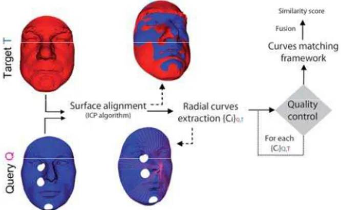
elastic shape analysis of radial curves [21]. As illustrated in figure 1, probe and gallery facial surfaces are first aligned using ICP algorithm; radial curves are then extracted from both surfaces; the corresponding probe and gallery curves are then compared within a Riemannian framework, and finally individual scores are fused to produce a general one which represent the degree of similarity between probe and gallery facial surfaces.
Figure 1: Block diagram of the studied 3D face rec. method
Within the proposed approach, the authors introduce a quality inspection filter that examines all the extracted radial curves in both gallery and probe models and retains valid ones based on the defined criterion.
3.1.1 Radial curves extraction
The reference curve is chosen to be the vertical curve once the face has been set into the upright position. Each radial curve βα is obtained by slicing the facial surface by a plane Pα with the nose tip as its origin, and which makes an angle α with the vertical plane. That is, the intersection of Pα with S gives the radial curve βα. This step is repeated to extract radial curves, indexed by the angle α, from the facial surface at equal angular separation. Figure 2 shows examples of some radial curves extraction under different quality degradations.
Figure 2: Examples of 3D faces with radial curves under different quality degradation
3.1.2 Radial curves matching framework
The Square-root velocity function is a specific mathematical representation (SRVF), denoted by q(t), used by the authors to analyze the shape of radial curves. It is
denoted according to:
q t
(4)
It has been shown in [10] that the classical elastic metric for comparing shapes of curves becomes the L2-metric under the SRVF representation. The collection of normed SRVF defines the pre-shape space set:
C q: | q I,
(5) The geodesic length between any two points q1, q2Є C is given by:
d q , q cos q , q
(6) The framework allows one to compute geodesic paths denoting optimal deformations between individual curves. Therefore, these deformations are combined to obtain full deformations between faces.
Figure 3: Examples of geodesic paths between source and target
Shown in Figure 3 is an example of such geodesic path between source and target faces belonging to the same person under different expressions.
The missing data problem is addressed by a quality module that inspects the quality of curves, and discards them if needed. Authors report that, by elastically matching radial curves, deformations due to expression are tackled. Thus, this method is a hybrid approach in between a holistic one such as ICP and a SIFT local feature-based one such as the second expert, introduced in the following subsection.
3.2. MS-ELBP + SIFT
The second expert is based on Multi-Scale extended LBP (MS-ELBP) along with local feature SIFT-based matching as detailed in [11]. This expert first generates several 3D facial representations (MS-ELBP) which are followed by a local feature SIFT-based matching and score fusion. It does not require any registration for roughly frontal faces as the ones in the FRGC datasets.
3.2.1 LBP and its descriptive power of local shape variations
LBP, a non-parametric algorithm [12], was first proposed to describe local texture of 2D images. It has been extensively adopted for 2D face recognition in the last several years [13]. However, computationally simple and direct application of LBP on depth images results in unexpected confusion to similar but different local shapes. To address this problem, two complementary solutions
were considered. The first one aims at improving the discriminative ability of LBP with Extended LBP coding approach, and the other one focuses on providing a more comprehensive geometric description of the neighborhood by exploiting a Multi-Scale strategy.
3.2.1.1 Extended Local Binary Patterns
Instead of LBP, ELBP not only extracts relative gray value difference between the central pixel and its neighboring pixels provided by LBP, but also focuses on their absolute difference. Specifically, the ELBP code consists of several LBP codes at multiple layers which encode the exact gray value difference (GD) between the central pixel and its neighboring pixels. The first layer of ELBP is actually the original LBP code encoding the sign of GD. The following layers of ELBP then encode the absolute value of GD. Basically, each absolute GD value is first encoded in its binary representation and then all the binary values at a given layer result in an additional local binary pattern. As a result, when describing similar local shapes, although the first layer LBP is not discriminative enough, the information encoded in the other additional layers can be used to distinguish them. Experimentally, the number of additional layers was set to 4.
3.2.1.2 Multi-Scale Strategy
The ELBP operator is further extended with different sizes of local neighborhood to handle various scales. The local neighborhood is defined as a set of P sampling points evenly spaced on a circle of radius R that is centered at the pixel to be labeled. For each (P, R) couple and each layer of the ELBP approach, a face is generated regarding the corresponding decimal number of the LBP binary code as the intensity value of each pixel. Such an image is called a MS-ELBP Depth Face (DF). Hence, DFs contain many details of local shapes (Figure 4).
Figure 4: MS-ELBP-DFs of a range face image with different radii from 1 to 8 (from left to right).
3.2.2 SIFT based local feature matching
Once the MS-ELBP-DFs are computed, the widely-used SIFT based features [15] are extracted from each DF separately for similarity score calculation and final decision. Because MS-ELBP-DFs highlight local shape characteristics of smooth range images, many more SIFT-based keypoints are detected than those in the original range images. In [11] it is reported that the average
number of descriptors extracted from each of DFs is 553, while that of each range image is limited to 41.
Given the features extracted from each MS-ELBP-DF pair of the gallery and probe face scan respectively, two facial keypoint sets can be matched [15]. Here, NLi(P, R)
denotes the number of the matched keypoints in the ith layer of ELBP-DF pair, with a parameter setting of (P, R).
The similarity measure, NLi(P, R), is with a positive
polarity (a bigger value means a better matching relationship). A face in the probe set is matched with every face in the gallery, resulting in an n-sized vector. Each of these vectors is then normalized to the interval of [0, 1] using the min-max rule. Matching scores of all scales are fused using a basic weighted sum rule:
S ∑ w P, R N P, R (7) The corresponding weight, wLi(P,R), is calculated
dynamically during the online step using the scheme in[16]:
w P, R L P, R L P, R
L P, R L P, R
(8)
where the operators max1(V) and max2(V) produce the first
and second maximum values of the vector V. The gallery face image which has the maximum value in S is declared as the identity of the probe face image. Extended results and analysis are provided in [11]. As we can see, this method is a local feature-based approach which should make it more tolerant to occlusion and missing data.
3.3. Recognition via TPS Warping Parameters
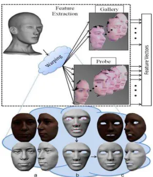
The third expert fits a generic model to facial scans in order to extract warping parameters to be used as biometric signatures. Face recognition based on morphable models has been extensively studied in the literature. A flexible model of an object class, which is a linear combination of the example shapes and textures, was introduced in [17]. Its extension to 3D was proposed in [18] and proved to give promising results. This expert makes use of a generic head model which is strongly deformed to fit facial models in the gallery, using the Thin Plate Spline (TPS) algorithm. Here, the aim is to utilize the discriminative properties of the warping parameters obtained during the fitting process.
TPS method was made popular by Fred L. Bookstein in 1989 in the context of biomedical image analysis [19]. For the 3D surfaces S and T, and a set of corresponding points on each surface, Pi and Mi respectively, the TPS algorithm computes an interpolation function f(x, y) to compute T’, which approximates T by warping S:
T x , y , z | x, y, z S, x x, y y, z f x, y (9)
f x, y a a x a y ∑ w |P x, y | (10)
When a generic model is deformed to fit an individual face in the database, an approximate representation of the facial surface is obtained. The deformation parameters represent the deviation from the generic face, and are therefore claimed to possess dense information about the facial shape.
Before TPS warping, a linear transformation is computed in a least square sense, based on 15 landmark points on both generic and inspected (target face) models. The obtained transformation which includes rotation, translation and isotropic scaling is applied onto the generic model. After that, in addition to the 15 point pairs utilized for alignment, 136 more pairs are generated, by coupling a set of points on the generic model with their closest neighbor on the target face. Using 151 point pairs in total, TPS interpolation is computed for the generic model.
Figure 5: The proposed feature extraction scheme and an illustration on a sample model: (a) Target face with and without texture (b) generic model before (with landmarks) and after alignment (c) generic model after warping with and without texture
Given in (10), the function f(x,y) includes the warping coefficients: wi, i={1,2,...n} to be utilized. When we transpose the formula for the other two directions, following feature vector is obtained: [(w1x,w1y,w1z), (w2x,w2y,w2z) …(w151x,w151y,w151z)]. The whole scheme is summarized in Figure 5, with an illustration on a sample model.
Once the feature vectors are extracted, Cosine and Euclidean distances are calculated between two warping vectors, resulting in two distance vectors of size 151x1. In order to measure the central tendency of these vectors,
trimmed mean approach is adopted and hence, sensitivity to outliers is avoided. For trimmed mean method, the portion to be ignored is taken as 10%.
3.4. ICP algorithm
In section 4, we also provide results of the baseline algorithm ICP as a comparison. Iterative Closest Point (ICP) algorithm [20] is a well-known reference algorithm in matching 3D point clouds through rigid transforms (translation, rotation). It is clearly a holistic matching algorithm in considering only rigid transforms. In our experiments, an automatic detection of the nose was applied, and the face was cropped with a sphere of radius 100 mm centered on the nose tip.
4. Experiments
As stated in the introduction, 3D models can suffer from various types of degradations having different origins. However, it is not easy to acquire a large dataset representing significantly these different degradations. A fundamental issue here is the quantification of degradations on real data. In this work, we decided to generate degraded data from the FRGC v2.0 dataset which is one of the most comprehensive dataset known so far in the literature. That choice allows us to have a large set of 3D face models under parameterized degradations, thereby testing the behavior of the experts and their fusion towards them. In this section, we first define the evaluation protocol then discuss the experimental results.
4.1. Experimental setup
The kinds of degradations that we consider are canonical ones as they typically occur in the acquisition process. They are Gaussian noise on depth, decimation in terms of resolution and holes for missing data.
410 subjects having more than one 3D face models were selected from the FRGC v2.0 database [3]. For each subject, one model with neutral facial expression was randomly picked to make up the gallery. We also randomly picked another model for each subject, which is used as a probe model. Before we could apply artificial, controlled degradations, we need to ensure that original 3D models are as clean as possible. Hence, gallery and probe sets were first preprocessed to remove spikes and holes as in [3]. Facial regions were further cropped from these gallery and probe sets based on the nose-tip within a sphere of diameter 100mm. For this purpose, nose-tips were manually located on every face.
From here, each cropped probe face model was then altered to some extent to create new, degraded sets, according to the following degradations:
- Gaussian noise corresponds to the injection of an error within a Gaussian distribution on the Z coordinates on
the depth image. This tends to emulate the behavior of electronic noise of acquisition devices, albeit a simplistic manner. In our experiments, we set the RMS value of the error respectively to 0.2, 0.4 and 0.8 (mm). - Decimation corresponds to removing vertices from the original data. In this experiment, vertices are picked randomly and removed respectively from a ratio of x2, x4 and x8.
- Holes are generated at random locations on the face. At first, we pick a random vertex on the surface of the face. Then, we crop the hole according to a 1 centimeter radius sphere centered on the latter vertex. For each level, we generate respectively 1, 2, 3 holes on the whole face.
Figure 6 shows examples of those degradations. In the subsequent, these three types of degradation are respectively denoted decimation (D), missing data (MD) and noise (N) having each three levels (2, 4 and 8). Each individual expert was then benchmarked on the subset of 410 subjects without degradations then using the previously defined degradations.
Figure 6: An example of degradations applied to one model. From left to right: the Original face, with Noise, Decimation, and Holes
As we will see in the following subsection, every individual expert displays different behavior in terms of performance drop against these degradations. Then, we further propose the fusion of these experts at score level, using the fusion scheme as described in section 2, thereby giving birth to several multi-matchers. The associated experimental protocol, as well as the performance of those multi-matchers, is detailed in subsection 4.2.2.
4.2. Results and Analysis
The performances of the four individual experts over the degradations are first analyzed. Then, our proposed fusion scheme (section 2) is compared to the standard sum rule fusion method [22].
4.2.1 Performances of the individual experts
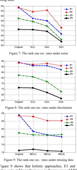
Recall that the four individual experts are: Expert using Elastic Shape Matching (E1), Expert based on MS-ELBP (E2), Expert using TPS (E3), ICP (E4). The 4 algorithms were benchmarked on the subset of 410 subjects as defined previously in subsection 4.1 and the various generated degradations. Figures 7-9 show the rank-one recognition rates of the four experts, respectively under noise (N), decimation (D) and missing data (MD). As we can notice,
all the algorithms record to some extent performance drops under degradations. While all the four algorithms resist relatively well to decimation and missing data, their performance drops drastically when the noise is increased to some level, 0.8 mm RMS in this work.
These results also suggest that the local feature-based expert, namely E2, displays the best robustness against the noise and decimation types of degradation. E1, a hybrid method, also displays a good behavior against decimation. Quite interestingly, the holistic approaches (E3 and E4) seem to behave better than other approaches against missing data.
Figure 7: The rank one rec. rates under noise
Figure 8: The rank one rec. rates under decimation
Figure 9: The rank one rec. rates under missing data
Figure 9 shows that holistic approaches, E3 and E4, display quite stable performance in the presence of MD.
4.2.2 Performances of multi-matchers
of facial surfaces, we further propose to study several multi-matchers, namely (1) E1+E2, (2) E1+E3, (3) E2+E3 and (4) E1+E2+E3, using the fusion scheme proposed in section 2. The 4th expert, based on ICP was considered as baseline. Since a learning dataset is needed to set the offline weights based on some global performance indicator of each expert, the whole dataset of 410 subjects was randomly divided into two equal parts, one part for learning and the other one for testing. This experimental setup was then cross-validated 50 times using each time different learning and testing data, and the performance averaged over these 50 cross-validations.
All the four multi-matchers were benchmarked on the degradations, namely decimation (D), missing data (MD) and noise (N) with the three levels (2, 4 and 8).
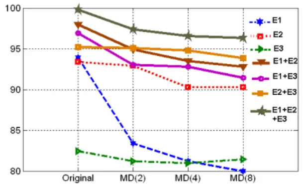
We experimented with three performance indicators, namely rank-one recognition rate (RR), verification rate at 0.1% FAR (VR) and Equal Error Rate (EER). The best performance being achieved using RR in the fusion scheme, we only report in fig.10, fig.11 and fig.12 the performance achieved by the four multi-matchers compared to the individual experts E1, E2 and E3 under different degradation scenarios and levels.
Figure 10: Rank-one Rec. Rate of the multi-matchers compared to the individual experts under different levels of noise
As we can see from fig.10, all the four multi-matchers display better performance under different level of noise, except once for E1+E3 on N(4), the best and stable performance being achieved by E1+E2+E3 which gives 99.77% recognition rate on the original data, 97.01%, 96.68% and 91.13% respectively under the three different noise level. This suggests that the fusion scheme has really capitalized on the complementary properties of individual experts. Notice also that E2+E3, which is the fusion of a local feature-based matcher (E2) with a holistic matcher through TPS (E3), outperforms E1+E2 and E1+E3 which are combinations of a hybrid method (E1) along with a local feature-based expert (E2) and a holistic expert (E3), respectively.
Fig.11 and Fig.12 further confirm the previous trend. Fig.11 gives the behavior of the four multi-matchers under different levels of decimation compared to the three
original experts. Once again, all the four multi-matchers display better and more stable performances than the three individual experts in almost all cases, the best performance still being achieved by E1+E2+E3 with 98.31%, 97.68% and 96.60% recognition rate respectively under decimation level 2, 4 and 8. The performance is thus only slightly decreased.
Figure 11: Rank-one Rec. Rate of the multi-matchers compared to the individual experts under different levels of decimation
Figure 12: Rank-one Rec. Rate of the multi-matchers compared to the individual experts under different levels of missing data
Fig.12 depicts the behavior of the four multi-matchers under different levels of missing data compared to the three original individual experts. Once again, all the four multi-matchers display better and stable performance than the three individual experts in almost all cases, the best performance being still achieved by E1+E2+E3 with 97.39%, 96.56% and 96.34% recognition rate respectively under missing data level 2, 4 and 8. As we can see, missing data only affects slightly the overall performance of the multi-matcher E1+E2+E3.
From Table 1, we can notice some performance improvements for the E1+E2+E3 multi-matcher (MM), compared to the standard sum rule (SS) and max rule (Max) fusion methods, for all the degradations at different levels. This proves that the proposed multi-matcher preserves the complementarity between all the experts. For the same experiment, the ICP algorithm seems to be more affected by decimation and Gaussian noise.
While the performances of our multi matcher are affected by degradations, this experiment shows that,
within a recognition scenario, it is more robust than any of the engaged individual experts to any type of degradation.
Table 1. Comparison between Rank-one Recognition Rate (%) of standard sum (SS) rule fusion method , max rule (Max) and our
multimatcher (MM) for the E1+E2+E3 (4)
SS Max MM SS Max MM N(2) 95.25 94.91 97.01 D(2) 95.60 95.22 98.31 N(4) 94.60 93.40 96.68 D(4) 94.50 94.37 97.68 N(8) 88.80 85.56 91.13 D(8) 94.20 93.73 96.60 SS Max MM MD(2) 95.40 95.07 97.39 MD(4) 94.83 94.18 96.56 MD(8) 94.50 94.41 96.34
5. Conclusion and Perspectives
In this paper, we discussed the robustness of four individual experts and their fusion with respect to three sample quality degradation scenarios, namely noise, decimation and missing data. The experimental results demonstrate that: (1) All the individual experts suffer somehow from sample quality degradations and display different behavior depending upon their intrinsic properties; (2) Globally, the performances are more affected by the presence of noise than by the presence of holes or decimation. (3) The multi-matchers using the proposed fusion scheme almost all perform better than individual experts under different degradation scenarios, thereby suggesting that the fusion scheme capitalizes on the individual expert strengths. Furthermore, the decrease in the performances due to quality degradations of the multi-matchers is less important than the decrease of each individual expert.
As a future development work, we would like to study the behavior of our multi matcher scheme against degradations within a verification scenario. This proposition suggests that the weight computation model has to be slightly modified.
References
[1] T. C. Faltemier. Flexible and Robust 3D Face Recognition Dissertation, University of Notre Dame, M.S., 2007. [2] I. A. Kakadiaris, G. Passalis, G. Toderici, M. N. Murtuza, Y.
Lu, N. Karampatziakis, and T. Theoharis: Three-dimensional face recognition in the presence of facial expressions: an annotated deformable model approach, PAMI, vol. 29, no. 4, pp. 640-649, 2007.
[3] P. J. Phillips, P. J. Flynn, T. Scruggs, K.W. Bowyer, J. Chang, K. Hoffman, J. Marques, J. Min, and W. Worek. Overview of the face recognition grand challenge. IEEE Intl. Conf. On Computer Vision and Pattern Recognition, 2005. [4] A. Colombo, C. Cusano, R. Schettini: Detection and
Restoration of Occlusions for 3D Face Recognition, IEEE International Conference on Multimedia and Expo, pp. 1541-1544, 2006.
[5] E. M. Bronstein, M. M. Bronstein, and R. Kimmel. Robust expression-invariant face recognition from partially missing data. In Proc. ECCV. 2006, Lecture Notes on Computer Science, pages 396–408. Springer, 2006.
[6] R. N. Rodrigues, L. L. Ling, V. Govindaraju. Robustness of multimodal biometric fusion methods against spoof attacks, Journal of Visual Language and Computing, doi:10.1016/j. jvlc.2009.01.010, 2009.
[7] N. Poh et al., Benchmarking Quality-dependent and Cost-sensitive Score-level Multimodal Biometric Fusion Algorithms, IEEE Transactions on Information Forensics and Security archive Volume 4 , Issue 4 (December 2009), Pages: 849-866, 2009.
[8] A. S. Mian, M. Bennamoun, and R. Owens. Face recognition using 2d and 3d multimodal local features. Intl. Symp. On Visual Computing, 2006.
[9] R. Snelick, U. Uludag, A. Mink, M. Indovina, and A. Jain. Large-scale evaluation of multimodal biometric authentication using state-of-the-art systems. IEEE Trans. on P.A.M.I., 27(3) : 450–455, 2005.
[10] S. Wang, Y. Wang, M. Jin, X. Gu, and D. Samaras. 3D surface matching and recognition using conformal geometry. In CVPR’06: Proceedings of the 2006 IEEE Computer Society Conference on Computer Vision and Pattern Recognition, pages 2453–2460, Washington, DC, USA, 2006. IEEE Computer Society. 12(1):234–778, 2002. [11] D. Huang, M. Ardabilian, Y. Wang, L. Chen. A Novel
Geometric Facial Representation based on Multi-Scale Extended Local Binary Patterns, IEEE Int. Conference on Automatic Face and Gesture Recognition, 2011.
[12] T. Ojala, M. Pietikäinen, T. Maenpaa. Multiresolution gray-scale and rotation invariant texture classification with local binary patterns, PAMI, vol.24, no.7, pp.971-987, 2002. [13] T. Ahonen, A. Hadid, M. Pietikäinen. Face recognition with
local binary patterns, ECCV, 2004.
[14] C. Shan and T. Gritti. Learning discriminative LBP-histogram bins for facial expression recognition, BMVC, 2008.
[15] D. G. Lowe. Distinctive image features from scale-invariant key-points, IJCV, vol. 60, no. 4, pp. 91-110, 2004.
[16] A. S. Mian, M. Bennamoun, and R. Owens, “Keypoint detection and local feature matching for textured 3D face recognition,” IJCV, vol. 79, no. 1, pp. 1-12, 2008.
[17] M. Jones, and T. Poggio. Model-based matching of line drawings by linear combinations of prototypes. In Proceedings of the Fifth International Conference on Computer Vision, pp. 531–536, 1995.
[18] V. Blanz, T. Vetter. Face recognition based on fitting a 3D morphable model. IEEE Transactions on P.A.M.I., vol.25, no.9, pp. 1063- 1074, Sept. 2003.
[19] F. L. Bookstein. Principal warps: Thin-Plate Splines and Decomposition of Deformations. IEEE Trans. on P.A.M.I., 11(6):567–585, June 1989.
[20] P. J. Besl and N. D. McKay. A Method for Registration of 3-D Shapes. Pattern Analysis and Machine Intelligence, Volume 14 Number 2, p. 239-255, February 1992.
[21] H. Drira, B. Ben Amor, M. Daoudi, and A. Srivastava, Pose and expression-invariant 3d face recognition using elastic radial curves. In Proc. BMVC, pages 90.1-11, 2010.
[22] A. Ross, K. Nandakumar, A.K. Jain. Handbook of Multibiometrics. Springer, Heidelberg (2006).