Recherche de séries temporelles à l’aide de DTW-preserving shapelets

HAL Id: tel-02510229

https://tel.archives-ouvertes.fr/tel-02510229

Submitted on 17 Mar 2020

HAL is a multi-disciplinary open access

archive for the deposit and dissemination of

sci-entific research documents, whether they are

pub-lished or not. The documents may come from

teaching and research institutions in France or

abroad, or from public or private research centers.

L’archive ouverte pluridisciplinaire HAL, est

destinée au dépôt et à la diffusion de documents

scientifiques de niveau recherche, publiés ou non,

émanant des établissements d’enseignement et de

recherche français ou étrangers, des laboratoires

publics ou privés.

DTW-preserving shapelets

Ricardo Carlini Sperandio

To cite this version:

Ricardo Carlini Sperandio. Recherche de séries temporelles à l’aide de DTW-preserving shapelets.

Machine Learning [cs.LG]. Université Rennes 1, 2019. English. �NNT : 2019REN1S061�. �tel-02510229�

L

’U

NIVERSITÉ DE

R

ENNES

1

COMUE UNIVERSITE BRETAGNE LOIRE

ÉCOLÉ DOCTORALE NO ₆₀₁

Mathèmatique et Sciences et Technologies de l’Information et de la Communication Spécialité : Informatique

Par

Ricardo C

ARLINI

S

PERANDIO

T

IME

S

ERIES

R

ETRIEVAL

U

SING

DTW-P

RESERVING

S

HAPELETS

Thèse présentée et soutenue à Rennes le 18 décembre 2019 Unité de recherche : IRISA — UMR6074

Thèse No_{: 00000}

Rapporteurs avant soutenance :

Dr. Florent MASSEGLIA Chargé de Recherche, INRIA, Montpellier Dr. Germain FORESTIER Professeur, Université de Haute Alsace

Composition du jury :

Attention, en cas d’absence d’un des membres du Jury le jour de la soutenance, la composition ne comprend que les membres présents

Président : Dr. Alexandre TERMIER Professeur, Université de Rennes 1

Examinateurs : Dr. Usue MORI Chercheuse, University of the Basque Country, Espagne

Dr. Florent MASSEGLIA Chargé de Recherche, INRIA, Montpellier

Dr. Germain FORESTIER Professeur, Université de Haute Alsace

Dir. de thèse : Dr. Laurent AMSALEG Directeur de Recherche, CNRS, IRISA, Rennes

Co-dir. de thèse : Dr. Guillaume GRAVIER Directeur de Recherche, CNRS, IRISA, Rennes Invités :

Dr. Silvio J. F. GUIMARÃES Professeur, Computer Science Department at PUC Minas, Brésil

Acknowledgements

The present document, results of four years of research, would not have been possible without the help, encouragements, and support of many persons. I thank all of them, and I present them all my gratitude.

I would like to thank Dr. Laurent Amsaleg and Dr. Guillaume Gravier, who directed my thesis. Laurent and Guillaume, thanks for providing me an opportunity to work on this exciting field, all their encouragement, considerations, and involvement at all times. The discussions, the insights, and all the rest of their support. Laurent, thank you for all the advice, encouragements, and tips. Aucun mot ne peut exprimer ma gratitude pour ce que vous avez fait, je vous remercie énormément.

I would like to thank Dr. Simon Malinowski for his contribution and support. Simon, your advises, and your previous work on time series and shapelets were of paramount importance in this thesis. Without his contribution, the achievement of this thesis would have been much more difficult. Je te dois une grande bière, Simon !

I would also like to extend special thanks to Dr. Silvio Guimarães and his team over the PUC/Minas. His friendship, suggestions, and advice were immeasurable. His participation in the jury of this thesis and his review of the text are highly appreciated too. Silvio, muito obrigado por tudo, você foi muito importante nestes anos.

I would like to thank Dr. Romain Tavernard for his collaboration and, especially, for the package TSLearn; with it, he helped me a lot, merci.

I would like to extend my gratitude to Professor Dr. Alexandre Termier for honoring my jury by presiding it. I also appreciate the participation of Professor Dr. Usue Mori (Université du Pays Basque), Professor Dr. Germain Forestier (Université de Haute-Alsace) and Professor Dr. Florent Masseglia (Université Montpellier 2), I appreciate the challenge they took in accepting to read my work. Thank you.

I would like to thanks Inria, IRISA and Université Rennes 1 for sheltering me during those years. Of course, I could not fail to thank Aurélie Patier, merci beaucoup Aurélie !

My sincere thanks to CNPq C onselho Nacional de Desenvolvimento Científico e Tecnolóógico (Pro-cess number 233209/2014–0) for providing the ne(Pro-cessary funds to develop this work.

Undoubtedly, I would like to thank my family, in particular, my wife Julia, for her never-ending support. Julia, I never dreamed that I’d meet somebody like you! And also to my little daughter Fernanda, who came to the world during this thesis and brought a new sense to my life. Fernanda, papai espera ter mais tempo para ti desde já. Amo vocês!

Finally, I would like to thank all the guys from the Linkmedia team, you guys have been a source of laughter and fun, and have helped me immensely and, I cannot thank you all enough.

Résumé Étendú

Il vaut mieux faire que dire. Alfred de Musset

Contents

Contexte . . . ix

Recherche en données temporelles . . . ix

Objectif et vue d’ensemble de la thèse . . . xi

Résumé des principales contributions . . . xv

Pistes pour des travaux futurs . . . xv

Contexte

La recherche scientifique traitant de l’analyse et de l’exploitation de séries temporelles est très active, notamment en raison de nombreuses applications telles que la surveillance des électrocar-diogrammes, la reconnaissance vocale ou la modélisation environnementale. Cette thèse s’inscrit dans cette veine et propose une nouvelle approche pour l’identification de séries temporelles similaires à une requête. Cette tâche est difficile pour plusieurs raisons.

D’abord, la fouille de données temporelles soulève de nombreux défis en raison de la spécificité des données manipulées. Les séries temporelles proviennent de mesures réelles et des séries temporelles ne différant que par des distorsions sur l’axe du temps ou par l’amplitude des valeurs enregistrées doivent être jugées similaires.

Ce résumé introduit les différentes problématiques abordées dans cette thèse. Dans un pre-mier temps, nous développons un court argumentaire afin de montrer l’intérêt de la recherche de séries temporelles. Puis nous développons les travaux réalisés dans le cadre du doctorat. Et enfin, nous présentons les résultats et les contributions obtenues.

Recherche en données temporelles

Une série temporelle, ou série chronologique, est une suite finie de valeurs numériques re-présentant l’évolution d’une quantité spécifique au cours du temps. Les données de séries chro-nologiques sont produites massivement 24 × 7 par des millions d’utilisateurs, dans le monde entier, dans des domaines tels que la finance, l’agronomie, la santé, la surveillance de la terre, les prévisions météorologiques, le multimédia, etc. En raison des progrès de la technologie des capteurs et de leur prolifération, les applications peuvent produire des millions à des milliards de séries chronologiques par jour, ce qui rend encore plus difficile l’extraction des données des séries chronologiques.

La fouille de données temporelles soulève de nombreux défis en raison de la spécificité des données des séries chronologiques. Les séries temporelles proviennent de mesures réelles et des séries temporelles ne différant que par des distorsions sur l’axe du temps ou par l’amplitude

des valeurs enregistrées doivent être jugées similaires. De nombreux facteurs peuvent produire ces distorsions, comme un capteur mal calibré ou imprécis, l’utilisation de différentes unités de mesure, ou le bruit, par exemple [EA12].

Cette thèse se concentre sur l’étude des mécanismes permettant de réaliser très efficacement des recherches de séries temporelles par similarité. Le scénario pour cette tâche est le suivant : soit τ une série temporelle de test (requête), la recherche consiste à identifier la série temporelle T∗parmi un ensemble de séries T appartenant à une base de données qui se trouve être l’élément plus proche de τ selon une mesure de la similarité D. En d’autres termes, il s’agit de trouver T∗_,

de telle sorte que :

T∗= arg min

Ti∈ T

D(τ ,Ti) (1)

Une méthode traditionnelle d’identification de T∗ _{repose sur le calcul par force brute de}

D entre τ et toutes les séries de T . Cette approche ne passe pas à l’échelle lorsqu’il s’agit de séries temporelles longues ou de bases de données énormes car calculer D est trop coûteux. Par conséquent, des méthodes doivent être employées pour réduire le coût de l’établissement de la similarité, comme s’appuyer sur l’indexation ou sur une approximation heuristique.

Initialement, comme dans d’autres domaines, la fonction D choisie pour mesurer la similarité des séries temporelles était une norme Lp, comme la distance euclidienne (Euclidean distance

(ED)). La mesure ED, en plus d’être rapide, est métrique, donc propice à l’indexation1_{. Toutefois,}

malgré ces avantages, la distance euclidienne ne donne pas de bons résultats avec les séries chronologiques car elle n’est pas robuste face aux distorsions sur l’axe du temps. Aussi, il est préférable de l’utiliser avec des données transformées ou d’utiliser une autre mesure plus robuste aux distorsions temporelles. Par conséquent, de nombreuses mesures de similarité et différents types de transformations de données ont été proposés pour les séries chronologiques, souvent destinés à résoudre des problèmes spécifiques à un domaine.

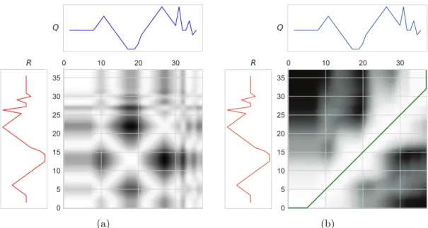
Parmi ces fonctions de distance proposées, une se distingue : l’alignement dynamique tem-porel, ou Dynamic Time Warping (DTW) [SC78]. La mesure DTW a la capacité de traiter les distorsions locales dans l’axe du temps, permettant un meilleur alignement entre les points des deux séquences, comme illustré par la Figure 1.

0

5

10 15 20 25 30 35 40

time

0

5

10 15 20 25 30 35 40

time

Figure 1 – (a) En utilisant l’ED, les deux séries temporelles ont une grande valeur de dissimilitude, contrairement à notre perception. (b) Un résultat plus intuitif est obtenu en utilisant DTW comme métrique pour la fonction de dis-tance D, en raison de sa capacité à gérer les distorsions locales de l’axe des

temps.

Cependant, la flexibilité de la DTW s’accompagne d’un coût de calcul quadratique [DTS+08]. Réduire la complexité de la DTW constitue l’objectif de nombreux chercheurs mettant au point de nombreuses optimisations élégantes, inventant des bornes inférieures de diverses nature ou concevant d’autres mécanismes [EA12]. Mais la quête de la meilleure performance dans le traitement de collections de séries temporelles extrêmement volumineuses est toujours active.

1_{Les distances métriques permettent d’utiliser l’inégalité triangulaire pour réduire le nombre de calculs dans}

D’autre part, une autre façon d’explorer le problème consiste à transformer l’ensemble de données et de lui donner une nouvelle représentation, en se concentrant uniquement sur les caractéristiques spécifiques de l’ensemble de données, réduisant ainsi sa complexité. Cette sim-plification permet l’utilisation de fonctions de distance plus simples et donc plus rapides.

La grande majorité de ces transformations exploite les caractéristiques globales de la série, telles que la transformation de Fourier discrète, ou Discrete Fourier Transformation (DFT) [FRM94 ; AFS93], pour citer un exemple. Cependant, la similitude basée sur la forme n’est pas toujours globale. Par exemple, considérons un électrocardiogramme (ECG) pour un patient dont l’aryth-mie à un seul battement est indicative d’un problème cardiaque. Si ceci était capturé comme une série temporelle et comparé à une série de comportements normaux, il serait difficile de détecter une différence en raison de la présence de nombreux battements cardiaques réguliers. La caractéristique discriminatoire, dans ce cas, serait décrite par la présence d’une petite forme locale dans la série indiquant un battement irrégulier, qui serait probablement manquée dans les domaines de la fréquence et du temps car la structure et la forme globale des données seraient encore très similaires.

Nous envisageons plutôt d’extraire de petites sous-séquences représentatives des séries chro-nologiques pour détecter les similitudes locales basées sur la forme entre les séries. Ces petites sous-séquences représentatives, connues sous le nom de shapelets, constituent un domaine im-portant de la recherche en fouille de données dans les séries chronologiques depuis sa proposition dans [YK09], et de nombreuses approches visent à étendre son application, pour accélérer son extraction ou même de redéfinir comment l’obtenir.

Parmi ces approches, une se distingue : la transformation à base de shapelets (Shapelets transform (ST) [BDHL12]). La ST utilise des shapelets pour créer une représentation vectorielle des séries temporelles, ce qui permet leur utilisation dans des algorithmes traditionnellement utilisés pour les données vectorielles. Toutefois, en général, les transformations à base de shapelets proposées dans la littérature sont des méthodes supervisées. Elles sont donc peu pratiques pour la tâche de recherche de séries chronologiques similaires, par nature non supervisée. La seule exception est l’approche d’apprentissage des shapelets préservant de la DTW (Learning DTW-preserving shapelets (LDPS)) [LMTA17].

La LDPS est la première approche de transformation de shapelet basée sur un apprentissage non supervisé. L’objectif n’est pas d’essayer d’apprendre des shapelets pour classes les plus discriminantes, mais plutôt d’apprendre des shapelets qui préservent au mieux la vraie mesure DTW dans le nouveau espace de plongement.

Dans cette thèse, nous proposons d’utiliser la LDPS comme base d’une système de recherche par similarité de séries temporelles (Time Series Retrieval (TSR)).

Objectif et vue d’ensemble de la thèse

C’est l’identification rapide de la ou ses séries les plus similaires à une série requête qui est sans aucun doute l’un des plus grands, sinon le plus grand, défi dans la recherche par similarité des séries chronologiques.

Dans cette thèse, nous essayons d’élucider une question : est-il possible de combiner la ro-bustesse aux distorsions selon l’axe temporel de la mesure DTW avec la vitesse de calcul de la mesure ED ? C’est pourquoi nous proposons une transformation qui réunit le meilleur des deux univers : la robustesse aux distorsions locales selon l’axe des temps, offert par la DTW, et la vitesse découlant de l’utilisation de la mesure Euclidienne.

Nous proposons ici une approche approximative pour la recherche de séries temporelles si-milaires fondée sur un changement de représentation au travers d’un processus de plongement. L’idée est de proposer une façon de transformer les séries chronologiques en représentations

vectorielles. Cette transformation est produite de manière à permettre qu’une recherche eucli-dienne puisse ensuite être appliquée efficacement entre les séries transformées afin de trouver le voisin le plus proche de la requête transformée que l’on veut identique à celui qui aurait pu être déterminé si l’on avait utilisé la mesure DTW. Naturellement, la transformation doit être soigneusement conçue pour que la recherche approximative soit précise. Un autre point crucial est lié au coût de calcul de la transformation. Au moment du test, la requête doit d’abord être transformée avant d’être comparée aux séries temporelles transformées de l’ensemble de données. La transformation ne doit donc pas être trop coûteuse.

Nous commençons par proposer l’utilisation de la LDPS pour la tâche de recherche par similarité, proposition nouvelle. Cette transformation est basée sur un apprentissage non super-visé telle que la distance euclidienne relative dans l’espace transformé reflète bien les mesures originales obtenues en utilisant la DTW.

Hors ligne, l’ensemble S avec d shapelets est appris de T , comme décrit dans [LMTA17]. Toutes les séries temporelles dans T sont ensuite transformées et forment T , qui est stocké dans une base de données.

En ligne, une série temporelle requête Tq est transformée en Tq en utilisant S. Les k voisins

les plus proches de Tq sont ensuite recherchés dans T et conservés dans une liste temporaire de

séries temporelles classées en fonction de leur proximité avec Tq.

Le résultat final peut ensuite être construit selon deux options : (a) la série temporelle brute associée au plus proche voisin trouvé dans l’espace transformé est considérée comme le plus proche voisin de la requête brute, ou (b) la vraie DTW est ensuite calculée entre la requête brute et les versions brutes des k séries temporelles transformées et identifiée, puis la série la plus proche selon la DTW est retournée.

Ce plongement préservant la DTW est tel que le classement dans l’espace transformé est une approximation du classement qui serait produit dans l’espace d’origine conformément à la mesure DTW. Cependant, ce classement basé sur L2 est obtenu beaucoup plus rapidement car

les distances euclidiennes sont moins coûteuses à calculer que les mesures DTW.

Nous savons qu’une transformation d’une série chronologique a un coût, c’est pour cela que dans la tâche de la recherche de séries similaires un compromis entre la qualité de la réponse et le temps de transformation doit être atteint. Dans le cas de la LDPS, le coût de transformation est lié au nombre de shapelets utilisées lors de la transformation. Par conséquent, notre objectif est d’obtenir une transformation qui utilise le moins de shapelets possible tout en préservant au maximum l’acuité de la réponse.

Ainsi, au lieu d’utiliser S comme spécifié par [LMTA17], il peut être préférable de conserver et d’utiliser pour la transformation uniquement un sous-ensemble de shapelets constitué d’éléments soigneusement sélectionnés.

Pour appliquer l’esprit des algorithmes de sélection de caractéristiques au cas d’une trans-formation de shapelets, il est nécessaire de définir : (a) une métrique afin d’évaluer la qualité respective de chaque sous-ensemble de shapelets, (b) une stratégie pour construire des sous-en-sembles de shapelets de plus en plus importants, (c) un critère d’arrêt interrompant la recherche de sous-ensembles plus grands.

Nous détaillons maintenant ces trois points.

Métrique d’évaluation pour comparer les sous-ensembles de shapelet et

pour le choix des sous-ensembles

Nous commençons par construire S comme spécifié dans [LMTA17]. Il n’est pas utilisé pour transformer des séries temporelles dans T mais plutôt comme un réservoir dans lequel seront ensuite piochées les shapelets les plus utiles.

Pour comparer les performances de différents sous-ensembles de shapelet, nous avons besoin d’une vérité terrain basée sur la vraie distance DTW entre les séries chronologiques. Pour la construire, la DTW entre toutes les paires de séries temporelles dans l’ensemble d’apprentissage de T est calculée et nous enregistrons pour chaque série temporelle l’identifiant de son plus proche voisin. Cet ensemble d’entraînement est ensuite divisé en 10 parties, dont 9 sont utilisées pour les tâches d’entraînement détaillées ci-dessous, l’une étant utilisée pour la validation, dans un contexte classique de validation croisée.

Ensuite, nous sélectionnons d′_{shapelets dans S et utilisons ces d}′_{shapeletspour transformer}

toutes les séries temporelles appartenant à ensemble d’apprentissage courant. En utilisant les mêmes d′ _{shapelets, nous transformons également chaque série temporelle de l’échantillon de}

validation et nous les utilisons en tant que requêtes.

Les séries temporelles transformées à partir de l’échantillon d’entraînement sont ensuite classées avec leur distance L2 à chaque requête. Il est donc possible de déterminer à quel rang

correspond la série chronologique vraie la plus proche pour cette requête. Nous répétons cette opération pour toutes les séries temporelles de validation et pour tous les échantillons. Cela revient à construire un histogramme des rangs où le vrai voisin le plus proche basé sur DTW apparaît.

Nous utilisons cet histogramme pour construire une fonction de distribution cumulative, puis nous calculons l’aire associée sous la courbe de cette fonction (area under the curve (AUC)). Nous considérons cette valeur de l’AUC comme la mesure de la performance permettant d’évaluer la qualité d’un sous-ensemble de shapelet. Plus cette AUC est élevée, meilleur est le sous-ensemble de shapelet. Cette métrique est bien adaptée à la tâche d’extraction du plus proche voisin car elle favorise le classement élevé du voisin le plus proche vrai dans la liste approchée.

La métrique étant définie, nous utilisons ensuite un algorithme glouton pour choisir les shapelets, en commençant par une liste vide. Nous y ajoutons la meilleure shapelet, puis la meilleure paire étant donné le choix fait plus tôt, etc.

Nous définissons quatre critères d’arrêt différents, qui déterminent quand arrêter d’ajou-ter des shapelets à l’ensemble actuel des shapelets sélectionnées, allant d’un choix minimal de shapelets à l’utilisation de toutes :

• DPSRg: Les shapelets sont ajoutées une à une jusqu’à ce qu’il ne reste plus de shapelets.

À la fin, le sous-ensemble qui conduit à la meilleure AUC globale est sélectionné.

• DPSRt: Nous calculons le gradient normalisé entre l’AUC du sous-ensemble actuellement

sélectionné et celle obtenue en ajoutant la shapelet qui améliore le mieux l’AUC. Si cette gradient est inférieure à 1, la sélection de shapelet est arrêtée.

• DPSRl: La sélection de shapelet est arrêtée dès que l’ajout d’une shapelet n’améliore pas

la valeur de l’AUC.

• DPSRf: utilise toutes les shapelets.

La Figure 2 affiche les valeurs de l’AUC à chaque itération de l’algorithme de sélection de shapelet sur l’ensemble de données Ham (à partir de l’archive UCR-UEA [CKH+15]).

Dans la littérature sur la sélection des caractéristiques, la méthode de sélection décrite ci-dessus peut être classée dans la classe wrapper, où un algorithme d’apprentissage est appliqué pour évaluer la qualité respective de différents sous-ensembles de caractéristiques, de manière itérative. Cette approche est la plus courante et, malgré son amélioration par rapport à la recherche exhaustive, elle reste un processus très coûteux pour l’analyse de nombreuses caracté-ristiques. Par conséquent, le filtrage précoce des caractéristiques non pertinentes ou redondantes améliorerait la vitesse de l’algorithme de sélection de caractéristiques puisqu’il y en aurait moins à analyser. Ceci est illustré par la Figure 3.

Les filtres sont généralement peu coûteux et rapides, et appliquent souvent une analyse statis-tique de base sur l’ensemble des caractérisstatis-tiques. Le filtre proposé ici repose sur la construction

10

50

100

170

Dictionary size

0.850

0.875

0.900

0.925

0.950

0.975

AUC

Ham

DPRS

LS

DPSR

DPSR

DPSR

DPSR

0 5 10 15 20 25 30 35

Dictionary size

0.850

0.875

0.900

0.925

0.950

0.975

AUC

Ham

DPRS

LS

DPSR

DPSR

Figure 2 – (a) : Comparaison des valeurs de l’AUC pour la sélection des caractéristiques basée sur le DPSR et le score laplacien.(b) : Zoom sur (a)sur

les 35 premiers éléments du dictionnaire.

Classificateur Sk S Algorithm S1 S2 ... Wrapper _S5 S2 Sc ... S de recherche (a) Sk Filter S1 S2 ... S5 S2 Sc ... S S (b)

Figure 3 – (a) La procédure du modèle wrapper. (b) La procédure du modèle filter.

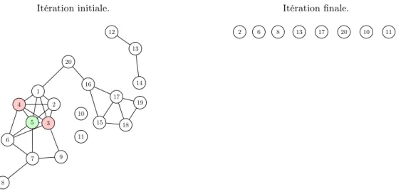
d’un graphe de shapelets basé sur la corrélation de Pearson, puis trouve des cliques dans ce graphe. Une seule shapelet par clique est conservée, les autres étant filtrées, comme indiqué dans la Figure 4. Itération initiale. 12 13 14 15 16 17 18 19 20 10 4 5 6 3 9 7 1 2 8 11 Itération finale. 13 17 20 10 2 6 8 11

Figure 4 – Nous commençons par un graphe fragmenté et finissons par un graphe totalement déconnecté.

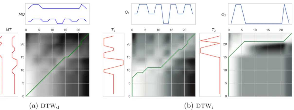
Les algorithmes DPSR et de filtrage décrit ci-dessus peuvent être étendus pour fonctionner avec des séries chronologiques à plusieurs variables. Pour étendre le DPSR (et le LDPS) aux séries multidimensionnelles, trois approches ont été proposées :

(i) M-DPSRi : independent multivariate DPSR : La première variante consiste à appliquer

M fois l’algorithme de [LMTA17] pour apprendre M dictionnaires indépendants, un par dimension de la série chronologique multivariée à transformer.

(ii) M-DPRSd: dependent multivariate DPSR : La seconde variante apprend un ensemble de

shapelets multidimensionnels.

(iii) M-DPSRs : slack multivariate DPSR : La troisième variante apprend un ensemble de

shapelets multidimensionnels, comme avec M-DPSRd. Mais c’est la transformation qui

diffère : La fenêtre coulissante du shapelet n’est pas rigide entre les dimensions.

Des expérimentations démontrent les bonnes performances de nos propositions, des tests statistiques ont montré que DPSR est significativement meilleur que PAA et LB_Keogh.

Résumé des principales contributions

Dans ce manuscrit, nous avons fait quatre contributions importantes :

(i) il explique comment les shapelets préservant de la DTW peuvent être utilisées dans le contexte spécifique de la récupération des séries temporelles

(ii) il propose quelques stratégies de sélection de shapelets pour faire face à l’échelle, c’est-à-dire pour faire face à une collection massive de séries temporelles ;

(iii) il présente un nouveau filtre multidimensionnel pour la sélection non supervisée de carac-téristiques ;

(iv) il explique en détail comment traiter les séries chronologiques univariées et multivariées, couvrant ainsi tout le spectre des problèmes de recherche de séries chronologiques. Le coeur de la contribution présentée dans ce manuscrit nous permet d’arbitrer facilement entre la complexité de la transformation et la précision de l’extraction.

Des expérimentations à grande échelle ont été menées à l’aide des archives de classification des séries chronologiques UCR [CKH+15] et des plus récentes archives de classification des séries chronologiques multivariées UEA [BDL+18], pour appuyer cette thèse et démontrer les importantes améliorations de performance par rapport aux techniques de pointe.

Pistes pour des travaux futurs

Dans cette thèse, nous avons montré que les shapelets pourraient aider à représenter des don-nées pour la recherche, en particulier après le choix d’un sous-ensemble approprié. La prochaine étape directe consiste à s’intégrer à un système d’indexation, à explorer l’inégalité triangulaire, évitant ainsi les calculs exhaustifs de la distance euclidienne et à améliorer davantage les perfor-mances. Une telle approche peut être avantageusement utilisée pour l’indexation à tout moment de séries temporelles.

Notre approche impliquant des shapelets préservant de la DTW montre des résultats très pro-metteurs, tant pour les tâches univariées que multivariées. Cependant, une question ouverte est d’améliorer l’apprentissage des shapelets originellement décrit par Lods et al. dans [LMTA17]. Cette approche privilégie la prise en compte de distances moyennes, sans s’attacher à préserver plutôt les distances aux k premiers éléments, ce qui est plus pertinent pour la recherche des séries temporelles similaires à une requête. Nous entrevoyons deux adaptations de l’algorithme LDPS. L’une consisterait à ajouter un mécanisme permettant de choisir les top-k shapelets au cours de la phase d’apprentissage. L’autre consisterait à modifier la fonction de perte afin qu’elle soit minimisée pour ne pas conserver les distances moyennes DTW mais plutôt les k premiers rangs.

Summary

Acknowledgements vii

Résumé viii

Résumé Étendú ix

Contexte . . . ix

Recherche en données temporelles . . . ix

Objectif et vue d’ensemble de la thèse . . . xi

Résumé des principales contributions . . . xv

Pistes pour des travaux futurs . . . xv

1 Introduction 19 Doing Data Mining with “Time” . . . 21

Contributions . . . 23

Organization . . . 24

2 Technical Background and Related Work 25 2.1 Basic Definitions and Notations . . . 25

2.2 Time Series Retrieval . . . 30

2.3 Data Representation and Distance Functions . . . 33

3 Time Series Retrieval Using DTW-preserving Shapelets 59 3.1 Overview . . . 60

3.2 Ranking and Selecting Shapelets . . . 62

3.3 Filtering Out Irrelevant Shapelets . . . 66

3.4 Extending to Multivariate Time Series . . . 74

4 Experiments 79 4.1 Datasets . . . 79

4.2 Experimental Setup . . . 81

4.4 Shapelet Selection Strategies for DPSR . . . 83

4.5 Filtering out Before Selecting . . . 84

4.6 Feature Selection vs. Instructed Feature Learning . . . 85

4.7 Multivariate Transformation versus Accuracy . . . 87

4.8 Selection, Filtering for M-DPSR . . . 87

4.9 Comparing Methods at Their Best for Multivariate Data . . . 88

4.10 Search Costs on Multivariate Data . . . 89

4.11 Discussion . . . 89

5 Conclusions and Perspectives 93 5.1 Results Summary . . . 93

5.2 Future Work and Extensions . . . 95

Contents 97

List of Figures 99

List of Tables 101

List of Algorithms 103

List of Abbreviations 105

A Specifications per Datasets 109

B Results on Univariate Dataset 113

C Results on Multivariate Dataset 121

Appendices

109

Bibliography

127

Bibliography 127

Chapter 1

Introduction

Begin at the beginning, the King said gravely, “and go on till you come to the end: then stop.” Lewis Carroll, Alice in Wonderland

Contents

Doing Data Mining with “Time” . . . 21 Contributions . . . 23 Organization . . . 24

From the earliest days, even before the development of the writing, the humans had already started to store knowledge (and data) by painting or sculpting in rocks and caves1_{. Now, after}

centuries of innovations, improvements in technology and gains in knowledge, humanity has reached a point where we can create 2.5 Quintilian bytes of data every day [Clo17], and there is nothing to indicate that this production will slow down.

(a) (b)

Figure 1.1 – Examples of human storing data: (a) The oldest known human preserved data: A figurative painting dated as over 40,000 years old, “stored” into the Lubang Jeriji Saléh cave. It is believed to be the representation of decapitation of a 1.5-meter-banteng bull [ASO+18]. (b) One of the dozens of Facebook’s data-centers, this in Sweden. On those servers, even the tracking

of the Facebook users’ mouse movement is stored.

Storing large amounts of data brings some challenges concerning hardware boundaries, where limitations are mainly encountered in issues such as cost, capacity, and bandwidth limits. How-ever, our biggest challenge lies in how to handle automatically and extract knowledge from this large volume of data. If for many years the manual extraction of patterns from collections of

the dataset was sufficient, since the Information Age2_{, due to the growth of dataset’s size and}

complexity, this process needs to be performed by computers.

The process of discovering patterns in large data sets is named Data mining (DM), and it involves methods at the intersection of statistics, Machine learning (ML), and database sys-tems [KDD06]. Algorithms for Data mining can be classified into three main groups:

Supervised algorithms: in this approach, the algorithm learns on a labeled (training) dataset. The supervised algorithm, using this provided training dataset, tries to model relationships and dependencies between the input data and the target prediction output (ground truth). Such that we can predict the output values for new data based on those relationships which it learned from the training dataset. The mass of practical machine learning uses supervised learning.

Unsupervised algorithms: The goal is to model the underlying structure or the distribution in the data, concerning to learn more about the data. The dataset is provided without explicit instructions on what to do with it. As there is no ground truth element to the data, unsupervised learning is a task more difficult than supervised learning. Once, it is hard to measure the accuracy of an algorithm trained without the aid of labels. However, for many situations, acquiring labeled data is prohibitive, or even we do not know a priori what kind of pattern we are looking for on the data.

Semi-supervised algorithms: It is a hybrid approach between supervised and unsupervised approaches. It uses a training dataset with both labeled and unlabeled data. This kind of method is particularly useful when extracting relevant features from the dataset is difficult, and the labeling task is costly and time-intensive for experts.

Approaches designed for data mining, need not only to be effective but also efficient, as we need to deal between an acceptable time response and an adequate quality of the returned answer. Besides that, in data mining tasks, we are exposed to scale-related issues. Algorithms for data mining need to present excellent performance with minimal impact according to the size of the dataset or the complexity of the analyzed data, i. e. the data’s dimensionality. The complexity of the data imposes a new question: how to compare these complex data? The typical approach is to use distance functions to measure how similar (or dissimilar) are two objects. Nevertheless, the algorithms’ performance is directly influenced by the dimensionality of the data and the number of objects to compare. The problem is when increasing the dimensionality of the data (its complexity), the volume of the space where this data is represented increases so fast that the available data becomes sparse and the measure distance becomes meaningless. In high-dimensional data, there is little difference in the distances between different pairs of objects. Those phenomena are called the curse of dimensionality [Bel03].

Some possible ways to handle the curse of dimensionality and the scale of the dataset are: (i) the use of dimensionality reduction techniques; (ii) the use of data transformation; (iii) and the acceleration of massive distance computation when comparing sets of objects by the use of lower-bounding functions and data structures.

Conventional approaches for dimensionality reduction are based in feature selection or ex-traction, where, instead of working the raw data (all of its dimensions), only the relevant ones are preserved or extracted. Data transformation consists of using some transformation function, create a new representation for the raw data. Whereas, a lower-bounding function is about replacing a costly function by another less costly, which produces a good approximation of the real distance.

Data analyzed in data-mining-related tasks vary from long texts to video, passing trough audio, sequences, images, among others. Our interest is in a particular class of sequences, the time series (TS).

2_{The historical period in the 21st century characterized by the rapid shift from traditional industry that the}

Doing Data Mining with “Time”

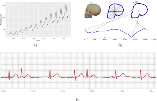
In a straightforward definition, time series is a special kind of data that represents a col-lection of values obtained from successive equally spaced measurements over time. However, this definition can be relaxed in such a way as to shelter in the “temporal-axis” other kind of measured sequences, like DNA or contours, among others. Figure 1.2 draws some examples of data represented as time series.

(a)

(i) (ii) (iii)

(b)

(c)

Figure 1.2 – Examples of time series: (a) The evolution and trend of the monthly air passengers. (b) A human skull is represented as a time series by firstly finding its outline (i). Then the distance from the center of the skull to each point on the skull’s outline is measured (ii). Finally, those distances are represented as a time series (iii). Lines are used to representing the relationship between the skull contours and the time series shape. In this case, we started at the skull’s mouth and went clockwise [KWX+06]. In (c), an ECG measured

by an Apple Watch.

Time series are massively produced 24×7 by millions of users, worldwide, in domains such as finance, weather forecasting, health, earth monitoring, agronomy, among others [EA12]. For example, in Figure 1.2, we can observe the monthly air passengers for a given time interval (fig. 1.2a), this is a common expected scenario for time series. In fig. 1.2b, we observe a time series where the time represents the position in the contours sequence. Moreover, finally, in fig. 1.2c, Electrocardiography (ECG) data captured using a personal device. Now, due to the proliferation of the Internet of Things (IoT), time-series data generation can grow exponentially. Time series can not only have a sizeable linear dimension (on the sense of its length along the time axis) but can also have more than one value varying over time. We call this case of time series as multivariate (or multichannel, or even multidimensional) time series. The adjective varies from the domain of study.

Therefore, algorithms need to be not only effective and efficient in dealing with temporal distortion but also when are vectors varying along the time.

Time Series Data Mining (TSDM) is a comprehensive research domain dedicated to the de-velopment of tools and techniques that allow the automatic discovery of meaningful knowledge

from time-series data. It provides techniques and algorithms to perform machine learning tasks on time series for assignments as diverse as classification, segmentation, clustering, retrieval, prediction, forecasting, motif detection, subsequences matching, anomaly detection, among oth-ers.

Time-series mining exists as a specific field because time series has its specifics properties and challenges. In particular, the meaningful information in the time series is encoded across the axis with trends, shapes, or subsequences usually with distortions. Also, this time-based factor not only makes it difficult but sometimes impossible to use data mining methods traditionally applied with massive success in other domains.

An interesting feature of time series analysis is that humans have an extraordinary capacity to visualize the shape of data, detecting similarities between patterns instantly [EA12]. Our ex-ceptional ability, delivered by the human neural cortex, allows us to ignore temporal distortions, noises, and enable us to deal with what is imperative, avoiding local fluctuations and noise in order to focus globally, and so, developing this overall notion of shape. Hence, time-series data mining emerges from the desire to materialize our natural ability.

For example, by giving an observed ECG from some patient, a medical doctor can make use of a time series retrieval system to look for some similar pattern in a time series ECG dataset. This retrieved information can help to provide the correct diagnoses.

Nevertheless, programming a computer to reproduce our natural capability is a hard prob-lem, and the difficulty arises in capturing the ability to match patterns with some notion of fuzziness [BC94]. According to Esling and Agón, these constraints show us that three major issues are involved:

(i) Data representation: How can the fundamental shape characteristics of a time series be represented?

(ii) Similarity measurement: How can any pair of time series be distinguished or matched? (iii) Indexing method: How should a massive set of time series be organized to enable fast

querying?

These implementation components represent the core aspects of the vast majority of time series data mining algorithms. Note that, due to their peculiarities, not all TSDM tasks require these three characteristics. For example, in forecasting, the notion of similarity is not necessary. Time series forecasting is more related to statistical analysis. If a few years ago, the omnipresent approaches were based in someway in flavours of Auto-regressive (AR) models, or Singular Spec-tral Analysis (SSA) [GAD+02], now deep neural networks, as Convolutional Neural Networks (CNN) or Long Short-Term Memory Networks (LSTM) models are dividing the attention.

On the other hand, tasks like classification, clustering, or retrieval are directly affected by how to assess similarity or how the data are represented. While in classification, the most common supervised task, for a given time series input, the classifier tries to identify what is the category of the input, based on learned data. In the clustering task, a traditional unsupervised approach, we want to identify groups of related time series without any previous knowledge about the data. In its turn, the retrieval task is based on the idea of given a query time series, search on a time-series dataset for the (group of) most similar time series to the query.

In common, for the three approaches previously cited, metrics to establish similarities be-tween time series are specific in the sense that they must be able to take into account the differences in the values making the series as well as distortions along the timeline. However, the retrieval task faces distinct challenges. Firstly, querying needs to be fast; thus, even the choice of the data transformation function is crucial. Second, it is common to handle the scale problem, which forces the use of optimized distance function, the choice of some data structur-ing. The comparison between pairs of time series can be dealt with by a more sophisticated measuring function; however, when the number of comparisons increases, we need to restrict the use of those complex functions.

Without any doubt, we can say that the most popular similarity measure is DTW. Nonethe-less, despite its ability in handling the notion of shape similarity, as we will see in Section 2.3.1.2, it is costly to compute, and using it against numerous or very long time series is difficult in prac-tice. Consequently, numerous attempts to accelerate the DTW were proposed; however, scaling the DTW remains a significant difficulty.

Working with raw time series is an arduous task, not only because of the dimensionality of its data but also due to the noise and temporal distortions. The presence of distortions makes unfeasible the use of less robust (and faster) similarity functions.

Therefore it is necessary to develop robust (and consequently computationally expensive) distance functions to deal with distortions or to define a new representation for the raw series, trying to preserve only the relevant information.

Luckily, one characteristic of the time series is that its consecutive values are usually not independent but highly correlated, thus with much redundancy. Such redundancy allows us to develop representation models that exploit these characteristics, such as correlation-based models or representations based on mean values.

A good representation is useful not only due to the data reduction, but it can also help in creating some transformation which allows the substitution of the costly DTW by a less expensive distance function with a minimal impact on the result’s quality.

Naturally, the quality of this representation largely depends on the embedding process. More-over, doing the right transformation, DM algorithms will not only be speed-up but can also produce better results than on the original data. Once the new representation will focus only on the relevant information, removing the noise and undesired parts of the data.

In this aspect, the family of contributions relying on the new concept of shapelets has proved to work particularly well. Originally proposed as a primitive for Time Series Classification (TSC), time series shapelets are phase-independent subsequences extracted or learned from time series to form discriminatory features. An evolution of the concept is to use shapelets to transform the raw time series in high-dimensional vectors and then use those vectors to feed a traditional machine learning classifier.

More recently, Lods et al. in [LMTA17] present the Learning DTW-preserving shapelets (LDPS), where they propose to embed the time series into a Euclidean space such that the distances in this embedded space well approximates the true measured by DTW. This work, focusing on the time series clustering, uses learned DTW-preserving shapelets to conduces the transformation.

In this manuscript, we propose the use of DTW-preserving shapelets for the specific context of large scale time-series retrieval.

We mainly focus firstly on developing the framework that can handle univariate and mul-tivariate time series. Then, we evaluate different approaches to handle mulmul-tivariate data-transformation. Thus, we propose how to evaluate the quality of a single shapelet and a set-of them. The challenge here is to define how good is a shapelet without any provided information. We have elaborated and developed a new method for feature selection based on clique-elimination, our method presented excellent results in our experiments, proving able to eliminate redundant information. All the proposed methods are evaluated with traditional benchmark datasets.

Contributions

This manuscript emphasized the representation of the information contained in the time series to support the retrieval task.

In this manuscript, we have made four significant contributions:

(i) it explains how DTW-preserving shapelets can be used in the specific context of time series retrieval;

(ii) it proposes some shapelet selection strategies in order to cope with scale, that is, in order to deal with a massive collection of time series;

(iii) it presents a new multidimensional filter for unsupervised feature selection;

(iv) it details how to handle both univariate and multivariate time series, hence covering the whole spectrum of time series retrieval problems.

The contribution’s core presented in this manuscript allows us to easily trade-off the trans-formation’s complexity against the retrieval’s accuracy.

Large scale experimentation was conducted using the UCR [CKH+15] time series classifi-cation archive and the newest UEA multivariate time series classificlassifi-cation archive [BDL+18], providing support for this thesis and demonstrating the vast performance improvements com-pared to state-of-the-art techniques.

Organization

As mentioned early, the purpose of this thesis is to bring new solutions for the time series retrieval problem. We have organized this manuscript in five chapters in order to fulfill this goal. Chapter 2 gives an overview of the notation and the concepts used in the manuscript and a thorough review of the state-the-art, from basic concepts to advanced algorithms for the time series retrieval is carried out. As we are proposing a new greedy-warping-like algorithm for selecting the best shapelets and also a clique-elimination-based filter approach for shapelet selection, a short revision in the feature selection domain is also necessary and done.

Next, in Chapter 3, we present our approach for TSR based on shapelet transformation, the DTW-Preserving Shapelet Retrieval (DPSR). This chapter also introduces our contribution to the work of Lods et al. We have generalized the LDPS to handle multivariate time series by proposing three new multivariate transformations. Besides, we will present our analysis of how to evaluate the quality of the learned shapelets in the original LDPS approach concerning the retrieval task. Based upon that analysis, we have proposed two new methods for feature selection: a greedy-based warp algorithm and a clique-elimination-based filter.

In turn, in Chapter 4, we use the proposed approach for DPSR on UCR time series classifi-cation archive and UEA multivariate time series archive, comparing the obtained results against two main competitors: the LB_Keogh lower bound (LB_Keogh) [Keo02] and the Piecewise Aggregate Approximation (PAA) [YF00; KCPM01]. The experimental result shows that DPSR can achieve a better retrieval performance on most datasets.

Chapter 2

Technical Background and Related

Work

We can only see a short distance ahead, but we can see plenty there that needs to be done. Alan Turing, Computing machinery and intelligence

Contents

2.1 Basic Definitions and Notations . . . 25 2.2 Time Series Retrieval . . . 30

2.3 Data Representation and Distance Functions . . . 33

This chapter gives an overview of the state-of-the-art Time Series Retrieval (TSR) algorithms, from basic concepts to advanced algorithms. First, we introduce notations and definitions related to TSR, and then we present the common distortions viewed in time-series data. TSR depends on how the implemented algorithms handle the distortions efficiently. Many algorithms use raw time series whereas others change the time series representation before the retrieval step. We thus categorize the different time series retrieval models that exist and review some of them with their most relevant characteristics. We start with the shape-based time series retrieval models, then we review the structure-based, finally we introduce the based on features. In this chapter, we only aim at categorizing the different types of time series retrieval algorithms as well as detailing the most famous and most competitive ones; and refer the curious reader to the numerous existing papers on this problem [YJF98; Fu11; RCM+12; EA12]. We conclude this chapter by briefly reviewing other Time Series Data Mining (TSDM) related to the retrieval task.

2.1

Basic Definitions and Notations

In the following, we provide definitions1 _{as well as useful notations in order to characterize}

the time series retrieval problem.

A time series is an ordered sequence of real values, resulting from the observation of an un-derlying process from measurements usually made at uniformly (time) spaced instants according to a given sampling rate [EA12].

In time-series data, the dependence between the N positions is induced by their relative closeness in the time-axis, that is, considering two possible positions nh and ni, they will often 1_{Although expressed primarily for the univariate case, such definitions are straightforwardly extended to the}

be highly dependent if |h − i| is small, with decreasing dependency as |h − i| increases [Jol02, p. 296]. A time series can gather all the observations of a process, which can result in a very long sequence. Also, a time series can result in a stream and be semi-infinite.

We can define a time series T as2

Definition 2.1 Time series. In a nutshell, a univariate time series (or only time series)T of length |T |= N is a sequence of real-ordered values typically collected in equally spaced intervals and formalized as:

T = {t1, t2, . . . , tN} (2.1)

whereti denotes theith _{element of the time seriesT .}

When the collected values are in a space RM _{such that M > 1, these time series are known}

as multivariate time series, sometimes called multidimensional or even multichannel.

Definition 2.2 Multivariate time series. A multivariate time series T is a set of M instances ofT ∈ RN univariate time series, expressed as:

T= {T1, . . . ,TM} ∈ RN ×M (2.2)

whereti, j is thejth element of theith channel of T.

For some application, it is more interesting to focus on the local shape properties of a time series rather than the global statistical properties, such as (global) mean, standard derivation, skewness, among others. These contiguous pieces of a long time series are called subsequences. Definition 2.3 Time series subsequence. Given a time seriesT of length N , a subsequence S ofT is a continuous sampling of T , with length |S |= l ≤ N , and starting at the position p of T , expressed as:

S= {tp, tp+1, . . . , tp+l−1} (2.3) where the valuep is an arbitrary position in T such that 1 ≤ p ≤ N − l+ 1.

Figure 2.1 draws an example of subsequence.

0 10 20 30 40 50 60 70 80 90 100

time

T S

Figure 2.1 – Illustration of subsequence S (in red) of a time series T .

Time series data mining related tasks suffer from the curse of dimensionality due to the high dimensionality of the data. Hence, it is common to work with a simplified representation of the series, defined as:

Definition 2.4 Time series representation. Given a time seriesT , with |T | = N , a represen-tation of T is a model T = {t1, . . . , tc} where c ≪ N , obtained by applying a transformation

function 𭟋 such that T = 𭟋(T ).

In general, besides the significant reduction of the data dimensionality, those transformations aims to emphasize fundamental shape characteristics or features, handling with noise and time-shifting.

For easier storage, massive time series-sets are usually organized in a dataset T .

Definition 2.5 Time series dataset. A time series dataset is a set of |T | = K unsorted time series, formalized as:

T = {T1, . . . ,TK} (2.4)

We will discuss some aspects of time series distortions in the following section, and after in the subsequent sections, we will present the methods for Time Series Retrieval (TSR).

2.1.1

Time Series Distortions

TSDM brings up many challenges due to the specificity of time series data. Time series comes from real-world measurements: even similar time series will present distortions on its time-axis or in the amplitude of its recorded values.

Many factors can produce those distortions, like a miscalibrated or inaccurate sensor, the use of different measurements units, or noise, for example [EA12]. In this section, we propose a brief overview of the commonly encountered in time series.

Distortion on Amplitude and Trend

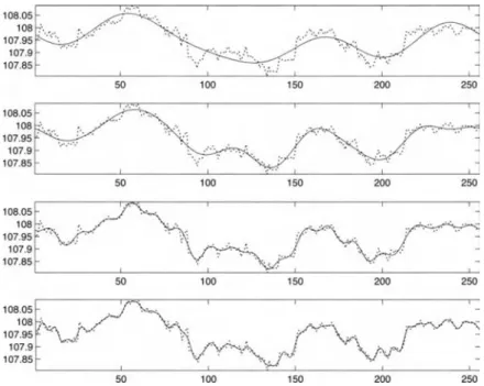
One common problem when dealing with time-series data is that they can present similar shapes while their values are on different scales. Many factors may influence the amplitude, for example, differences in the recorded volume (in the case of sound), illumination (image), data measured with different units like temperature measured in Fahrenheit or Celsius. Those factors can change the amplitude of the measured data while the intrinsic shape is comparable, therefore, if our interest is in looking for similarity on the shape, scaling the time series by removing the amplitude factor is a sine qua non condition.

Similarly, even if both time series have identical amplitudes, they may have different trends (or offset), in other words, it presents varying mean over time, and for some scenarios, the offset in the values (resulting from the trend) breaks the distance function. Similarly, even if both time series have identical amplitudes, they may have different trends (or offset); in other words, it presents varying mean over time. For some scenarios, the offset in the values (resulting from the trend) breaks the distance function. Some distance measures, such as the Euclidean distance, are sensitive to this family of distortion and fails to recognize the similarity of time series exclusively due to differences in the amplitude.

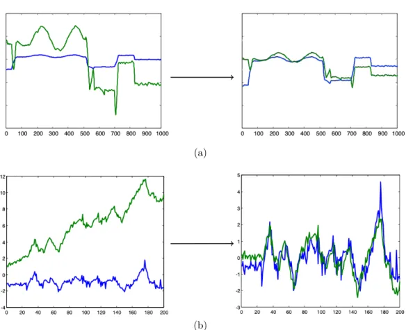
In this way, a usual pre-processing stage consists in applying a z-normalization to the data before evaluating the similarity, as illustrated in Figure 2.2a, or by scaling and removing the trend factor, as showed in Figure 2.2b.

(a)

(b)

Figure 2.2 – (a) Amplitude scaling: If compared before amplitude scal-ing (left), these time series appear very different. After applying the z-normalization, it appears more similar. (b) Applying the amplitude scaling plus offset translation and linear trend removal, allow to observe the similarity

Local Distortion on the Time-axis

As common as the previous case, however, more complex to be handled, we can visualize the local distortions on the time-axis as acceleration or deceleration in the phenomenon registered by the data points on the time series. Local distortion on the time-axis is the most common phenomenon handled in TSR and is showed in Figure 2.3.

Conventional approaches to handle this type of distortion are based on using a similarity function able to match non-aligned points between the sequences, i. e. , an elastic measure. Alternatively, creating a new representation focusing on the relevant features of the time series, and then doing the similarity evaluation on the transformed space.

Figure 2.3 – Local distortion on the time-axis: The lines represent the com-parison point-to-point. While in the traditional non-elastic measures (left) points are matched one-to-one, in the elastic measure, it allowed matching

one-to-many (right).

Distortion on Phase

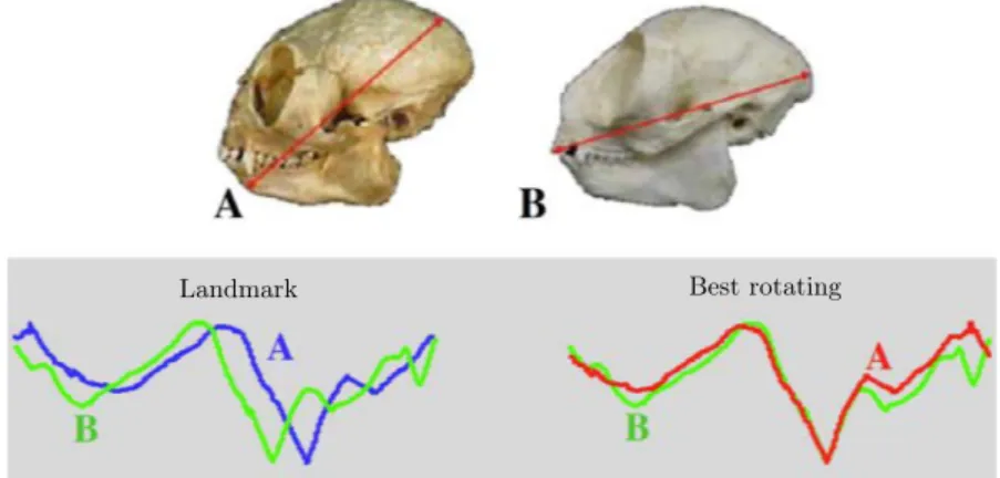
In some scenarios, the phenomenon of interest may be randomly positioned on the time series. For example, when using time series to represent a contour of a two-dimensional object, the starting point of the time series may not be adequately positioned causing a phase mismatch, as observed in Figure 2.4.

There are two solutions for this issue: either the whole time series are comparable and all the possible alignments must be tested [BKTdS14], or by using some representation based on feature extraction, and then doing the comparison on the transformed space.

Landmark Best rotating

Figure 2.4 – Phase distortion: Two primate skulls (A and B) represented as a time series of its contour. In the Landmark matching, the major axis is defined as the starting point (red line), phase distortion is observed and can conduce to incorrect similarity measure (left). Considering the best rotation,

Occlusion-based Distortion

This distortion occurs when small subsequence(s) of a time series may be missing or pre-senting an abnormal pattern. For example, some information can be lost while collecting or transmitting by a sensor, or it may be disturbed by some phenomena.

One way to handle occlusion-based distortion is allowing the elastic measure function to ignore sections (with the possibility of some penalty) that are difficult to match. Figure 2.5a shows a more visually intuitive example, where, probably, mutations throughout evolution have led to disturbances between the observed shapes.

Uniform Distortion on the Time-axis

Uniform distortion on the time-axis, in contrast to the localized distortion, can be seen as a case where the whole time series is uniformly warped in time. In other words, the time series is compressed or stretched, as showed in Figure 2.5b.

Methods proposed to handle local distortion does not perform well on a uniform distortion case. It is therefore preferable to re-scale one (or both) series before comparing them. However, the challenge in handling uniform scaling is that there is not an easy way to know the scale-factor before ahead.

(a)Occlusion. (b)Uniform scaling.

Figure 2.5 – Occlusion and uniform scaling distortions: (a) Occlusion distor-tion: The nose region of the ancient skull (bottom) has no correspondence and is missing on the modem skull (top). A way to out-pass this issue is ignoring the non-matching segment (blue arrow). (b) Distortion on uniform scaling: (I) Without any pre-processing, a full gene expression, CDC28, matches poorly to the prefix of a related gene, CDC15. (II) If it is re-scaled by a factor of 1.41, it matches CDC15 much more closely (III). Adapted from [BWK11; BKTdS14].

2.2

Time Series Retrieval

The retrieval task (or query by content) is the most active area of research in time series analysis [EA12]. It aims to locate objects in a dataset that are most similar to a query object Q provided by the user.

According if it handles or not the raw time series, retrieval can be classified in shape-based, structure-based or feature-based. Also, the queries can be called on complete time series (whole

matching) or to find every subsequence of the series matching the query (subsequence matching). In this thesis, we focus on feature-based whole-matching retrieval.

For the TSR task, the notion of similarity is a crucial concept, and the measurement of similarity between time series is a paramount subroutine not only for the TSR but also almost every TSDM task requires at least an indirect notion of similarity between pairs of time series. Its purpose is to compare two instances by computing a single value evaluating their similar-ity. A similarity (dissimilarity) measure is a real-valued function that measures how close (far) two instances are to each other. The closer the instances are, the larger the similarity is. There exists many (dis)similarity measures and definitions of it, amongst them we indicate a special case: distance metrics.

In the case of two time series Q and T with, respectively, length of NQ and NT, the distance

function D is defined as:

Definition 2.6 Distance between time series. D(Q,T ) is a distance function that takes time seriesT and Q as inputs and returns a non-negative value d, which is said to be the distance or (dis)similarity betweenQ and T .

The distance function D can also be used to measure the distance between two subsequences of the same length since the subsequences, in this case, can be viewed as an entire series. How-ever, we will also need to measure the similarity between a short subsequence and a (potentially much) more extended time series. We therefore define the distance between two time series T and S, with |S| ≪ |T | as:

Definition 2.7 Distance from a time series to the subsequence. subD(T , S) is a distance function that takes time seriesT and subsequence S as inputs and returns a non-negative value d, which is said to be the distance or (dis)similarity betweenT and S.

subD(T , S)= min (D(S, S′)) _{∀ S}′ ∈ S_T|S |, (2.5) where S_T|S | is the set of all possible subsequences inT with length |S |.

Based on the concept of similarity distance, we can define the time series retrieval task as follows:

Definition 2.8 Time series retrieval. Given a time seriesQ, the time series retrieval problem is to findT∗∈ T that is the most similar to Q according to the similarity measure D:

T∗= argmin

Ti∈ T

D(Q,Ti) (2.6)

We can generalize the previously definition to retrieval not only the closest element T∗_{, but}

also all elements inside an area defined by a threshold-range φ (Figure 2.6b) – φ-range retrieval, defined as:

Definition 2.9 Time series range search. Given a query time series Q, a time series dataset T , and a range threshold φ, the range search will return a subset R ⊂ T such that: R = {Ti ∈ T | D(Q,Ti)< φ}, for a given similarity measure D.

Or even the k-nearest neighbors (Figure 2.6c) – k-NN retrieval, defined as:

Definition 2.10 Time seriesk-nearest neighbors search. Given a query time series Q, a time series dataset T , and a integer k, the k-NN search will return a subset R ⊂ T , where the time seriesTk ∈ R are the k most similar to Q, according to the similarity measure D.

(a)

φ

(b) (c)

Figure 2.6 – Diagram of a typical query by content task represented in a 2-dimensional search space. Each point in this space represents a object whose coordinates are associated with its features. (a) A query object (orange point) is first transformed into the same representation as that used for other data points. Two types of queries can then be computed. (b) Aφ-range query will return the set of series that are within distanceφ of the query. (c) A k-nearest neighbors query will return thek points closest to the query, the yellow line

represents closest.

Figure 2.6 illustrates a typical query by content task in a 2-dimensional search space. In turn, subsequence retrieval requires searching all subsequences in the dataset, therefore, to compare a subsequence query C, |C| = l and a time series T , |T | = N , where l ≪ N , we need to extract all subsequences S ⊂ T with length l. We can obtain all subsequences by using a sliding window of the appropriate size.

Definition 2.11 Sliding Window. Given a time seriesT , |T |= N and a subsequence of length l, all possible subsequences of T can be extracted by sliding a window of size l across T and considering each subsequenceSlp. Here, the superscriptl indicates the length of the subsequence

and the subscriptp is the starting position of the sliding window over T . The set of all subsequences of length l extracted from T can be defined as:

Definition 2.12 Set of all subsequences of lengthl in T . Given a time series T , |T |= N and a subsequence of lengthl. The set of all subsequences of length l extracted from T is expressed by: S_Tl = {Sl_p of T , for 1 ≤ p ≤ N − l+ 1}. (2.7) We use Sl

T to represent the set of all subsequences of length L in the dataset T .

Although it seems trivial, the retrieval task faces numerous challenges, and due to many reasons depending on the data, this task is far from easy. The main challenges stem from:

(i) Even a time series considered short has dozens of positions on the time-axis. That is, time series is high-dimensional data.

(ii) Usually, on TSR tasks, the dataset is massive and needs to support adding and removing objects. Therefore, approaches for TSR need to work at scale in open datasets.

(iii) Surely the time series data in the dataset will present some distortion on the time-axis. Consequently, the similarity measurement function needs to be able to handle distortions. (iv) The query response time needs to be fast. Thus, the similarity function needs to be

effective in handling distortions but also efficient in doing it faster.

Three main ways were found out to handle those previously listed challenges. The first is defining similarity measure functions that are robust to time-axis distortions. The second is proposing data-transformation functions able to extract features expressing what “really means” in the time series data, and consequently mitigating the temporal distortions. Finally, the

combination of both, i. e. a transformation is applied to simplify the data together with a similarity function able to handle distortions.

In the following sections, we will present the most representative and used similarity measures and data transformations applied to time series retrieval.

2.3

Data Representation and Distance Functions

Data representation formats and distance functions are closely related to each other. There-fore, we are reviewing together current techniques on these two issues. Generally, we can classify these techniques into two main categories: distance functions on raw representations, or distance functions on data-transformed representations.

Following, we will discuss the characteristics of the main types of distance functions applied to time series. Our objective in this section is not to be exhaustive on time series distance measures but rather to give some instances of the preeminent families of distance measures: we encourage the reader to refer to dedicated surveys such as [DTS+08; WMD+13; KK03].

2.3.1

Distance Functions on Raw Representation

As previously defined in the Definition 2.1, a time series data can be represented as a sequence of real-ordered values, T = {t1, . . . , tN}. T is called raw representation of the time series data.

Many distance functions have been proposed based on raw representation.

The definitions of distance functions presented in this section use univariate time series data (M = 1) as an example, but they can be easily extended to multi-dimensional data.

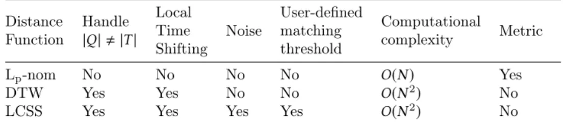
2.3.1.1 Euclidean Distances and Lp Norms

The Lpdistance family contains the most straightforward similarity measures for time series.

Also known as Minkowski distance, the Lpdistance corresponds to a family of functions, where

p ∈ R∗₊, and can be considered as a generalization of Manhattan (p = 1), Euclidean (p = 2), and Chebyshev (p = ∞) distances.

Given two time series T and Q of the same length N , the Lp-norm (or Minkowski) distance

between T and Q is:

L_p(T , Q)= ∥T − Q ∥_p= p   √ N ∑ i=1 |ti − qi|p (2.8)

Undoubtedly, the most known and most used distance measure is the Euclidean distance (ED) due to its simplicity to understand and effortlessness to compute. To compare the time series T and Q with the same length using the Euclidean distance, we compare each-other point-to-point, where the similarity is defined by:

D(T , Q)= L2(T , Q)=   √ N ∑ i=1 (ti − qi)2. (2.9)

Figure 2.7 shows a visual intuition of the Euclidean distance metric.

As in other data domains, the traditional Lp-norm have been the first choice to measure the

similarity in time series data [YF00; EA12]. It has the advantage of being easy to compute, parameter-free, and the computation cost is linear in terms of time series length. However,

Figure 2.7 – Viewing the Euclidean distance: The Euclidean distance between two time series can be visualized as the square root of the sum of the squared

length of the vertical hatch lines. Adapted from [BWK11].

unlike other data types where it achieves good similarity measure, on time series data Lp-norm

tends to lead results that do not reflect the human perception [DTS+08; EA12].

Humans have an extraordinary capability to observe similar patterns. The evolution brought us an ability to filter noise, phase shift, time distortions, scaling, amplitude, outliers allowing to focus essentially on the shape of the time series.

Therefore, it is evident that the simplicity of the Lp-norm fails to reach such level of

abstrac-tion, may causing then a totally unexpected similarity behavior.

We can resort a toy example to exhibit this phenomenon. Considering a time series dataset T = {Q, R,T } with |Q| = |R| = |T | = N , from Figure 2.8.

0 5 10 15 20 25 30 35 40 −4 −2 0 2 4 time Q

(a)Time seriesQ

0 5 10 15 20 25 30 35 40 −4 −2 0 2 4 time R (b)Time seriesR 0 5 10 15 20 25 30 35 40 −6 −4 −2 0 2 4 time T (c)Time seriesT

Figure 2.8 – Toy example of a time series dataset T with three time series.

Based on the behavior of our natural perception of shape, we believe that the pair (Q, R) is the most similar pair in T . However, the opposite is observed when we are using the L2-norm,

and this pair of sequences is considered the most dissimilar, as observed in Figure 2.9.

0 5 10 15 20 25 30 35 40 time (a)D(Q, R) = 19.3907 0 5 10 15 20 25 30 35 40 time (b)D(Q, T ) = 18.72357 0 5 10 15 20 25 30 35 40 time (c) D(T, R) = 18.6957

Figure 2.9 – The use of L2-norm as distance function D conduces to an unexpected measure of similarity. In this context, the pair (Q, R) (in (a)) is

evaluated as the least similar pair, contradicting the human perception.

Below we will show how other metrics can be used to mitigate this issue of the Euclidean distance.