Statistical Computing On Manifolds for 3D Face Analysis and Recognition

(1)

HAL Id: tel-00728009

https://tel.archives-ouvertes.fr/tel-00728009

Submitted on 4 Sep 2012

HAL is a multi-disciplinary open access archive for the deposit and dissemination of sci-entific research documents, whether they are pub-lished or not. The documents may come from teaching and research institutions in France or

L’archive ouverte pluridisciplinaire HAL, est destinée au dépôt et à la diffusion de documents scientifiques de niveau recherche, publiés ou non, émanant des établissements d’enseignement et de recherche français ou étrangers, des laboratoires

Statistical Computing On Manifolds for 3D Face

Analysis and Recognition

Hassen Drira

To cite this version:

Hassen Drira. Statistical Computing On Manifolds for 3D Face Analysis and Recognition. Computer Vision and Pattern Recognition [cs.CV]. Université des Sciences et Technologie de Lille - Lille I, 2011. English. �tel-00728009�

(2)

Ann´ee 2011 Num d’ordre: 40556 Universit´e Lille1

TH`ESE

pour obtenir le grade de Docteur,

sp´ecialit´e Informatique

pr´esent´ee et soutenue publiquement par

Hassen DRIRA

le 4 juillet 2011

Statistical Computing On Manifolds for 3D Face Analysis and

Recognition

pr´epar´ee au sein du laboratoire LIFL sous la direction de

Mohamed DAOUDI Boulbaba BEN AMOR

COMPOSITION DU JURY

M. Liming Chen (Professeur, Ecole Centrale de Lyon, France) Président M. Remco Veltkamp (Professeur, Université de Utrecht, Pays-bas) Rapporteur M. Pietro Pala (Associate Professor, Université de Florence, Italie) Rapporteur M. Anuj Srivastava (Professeur, Florida State University) Examinateur M. Mohamed Daoudi Professeur TELECOM Lille1/LIFL Directeur M. Boulbaba Ben Amor (Maˆıtre de conférences, TELECOM Lille1/LIFL) Encadrant

(3)

(4)

Acknowledgements

First of all, I would like to thank my thesis advisors for their trust, and more specifically for having made me discover scientific research and the two research fields of top excitement that are Shape Analysis and Biometric. During these three years, Pr. Mohamed Daoudi has been a mentor to me, even more than at a pure scientific level. I would like to express my gratitude to Dr. Boulbaba Ben Amor for his outstanding human qualities and its unconditional encouragements which definitely helped me mutate into a grown-up researcher. I would also like to thank Pr. Srivastava, who has provided me with insights into the research process, and for inviting me during two mouths in his laboratory.

A special thanks is due my PhD committee members for taking the time to participate in this process, and especially the reviewers of the manuscript for having accepted this significant task: M. Pietro Pala (Associate professor at University of Florence) and M. Remco Veltkamp (Professor at University of Utrecht) and kindly accepted to sacrifice their precious time for the manuscript reviewing.

I also thank the committee members M. Liming Chen (Professor at Ecole Centrale Lyon) and M. Anuj Srivastava (Professor at Florida State University). All these people made me the honor to be present for this special day despite their highly charged agendas and Im sincerely grateful for that.

A special thank goes to my research buddies and especially master students Rim Slama and Eric Foe for their help.

I thank my family, my friends, people at TELECOM Lille 1 and LIFL for their never decreasing warm encouragements. Finally, I d like to thank my wife Emna and my parents Abdelaziz and Najet, whose support of my graduate career has helped me to endure the marathon of the PhD process.

(5)

(6)

List of figures

1.1 bloc diagram of the project tasks. . . 16 2.1 Output of the 3D sensor: range and color image at top row and 3D mesh

with and without color mapped on in bottom row. . . 23 2.2 Example of face from FRGCv2 face. 3D data is shown at top and the texture

is mapped on it at the bottom. . . 24 2.3 Examples of all 3D scans of the same subject from GAVAB dataset. . . 24 2.4 Examples of faces from the Bosphorus and illustration of the problems of

incomplete data (due to the pose or occlusion) and deformations of the face (due to expressions). . . 25 2.5 3D face model and different representations: point cloud and 3D mesh. . . . 26 2.6 Deformations under facial expressions (a). Missing data due to self occlusion

(b). . . 28 2.7 Euclidean path (in red) and geodesic one (in blue) on facial surface . . . 29 2.8 Points correspondence (neutral face at left and expressive face at the right) 31 3.1 An illustration of challenges in facial shape in presence of large expressions.

The level curves of geodesic distance to the nose tip lying in regions outside the nose are significantly distorted while the curves in nose region remain stable. . . 41

(11)

LIST OF FIGURES

3.2 Histograms of distances (for some level curves) between different sessions of

the same person . . . 42

3.3 Automatic FRGC data preprocessing and nose curves extraction. . . 44

3.4 Automatic nose tip detection procedure. . . 45

3.5 Examples of pre processed data: nose region with geodesic level curves . . . 46

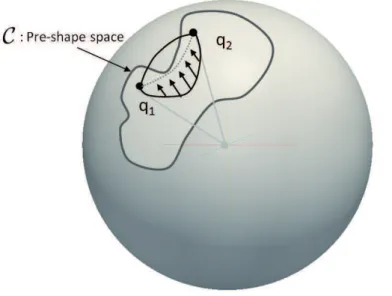
3.6 Illustration of the Pre-Shape Space C and geodesic in this pre-shape space. 48 3.7 Examples of geodesic between curves . . . 50

3.8 Computing geodesics in the quotient space. . . 51

3.9 Geodesic path between source and target noses (a) First row: intra-class path, source and target with different expressions (b) Three last rows: inter-class path . . . 52

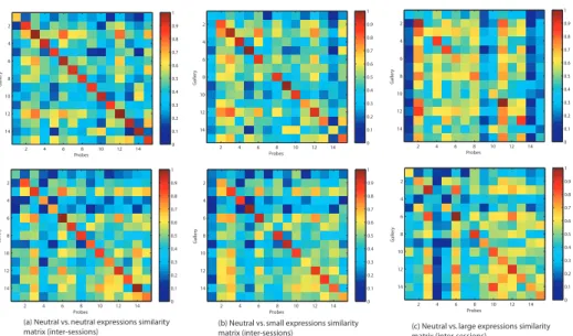
3.10 Similarity matrices for (a) neutral vs. neutral comparsions, (b) neutral vs. small expressions, and (c) neutral vs. large expressions, top row includes marices for face-to-face matching and buttom row includes nose-to-nose matching. . . 54

3.11 Rank one recognition rates using 1 to k curves . . . 55

3.12 Verification Rate at FAR=0.1% using (1 to k) curves . . . 56

3.13 ROC curves using 1 to k curves . . . 57

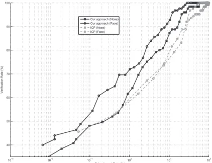
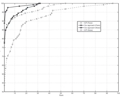
3.14 Receiver operating characteristic curves for our approach and ICP (baseline) 58 3.15 Cumulative Match Characteristic curves for our approach and ICP (baseline) 59 3.16 Examples of noses that are recognized by our approach and not by ICP algorithm on nose region . . . 62

3.17 Examples of noses that are not recognized by our approach . . . 63

4.1 Important challenges of 3D face recognition. (a) neutral face, (b) expression variations, (c) missing parts due to scan technology and pose variation, (d) pose and expression variations . . . 66

4.2 Significant changes in both Euclidean and surface distances under different face expressions. . . 67

(12)

LIST OF FIGURES

4.3 Overview of the proposed method. . . 69 4.4 Different steps of preprocessing: acquisition, filling holes, cropping and

smoothing . . . 70 4.5 Radial curves extraction : left image illustrates the intersection between the

face surface and a plan to form two radial curves. The collection of radial curves is illustrated at the right image. . . 71 4.6 Illustration of elastic metric. In order to compare the two curves in (a),

some combination of stretching and bending are needed. The elastic metric measures the amounts of these deformations. The optimal matching between the two curves is illustrated in (b). . . 72 4.7 An example of matching of two radial curves extracted from two faces. a)

A curve on an open mouth, (c) a curve on closed mouth , b) change of parametrization before matching . . . 76 4.8 Illustration of shape space and geodesic between its elements. . . 77 4.9 An example of matching and geodesic deforming radial curves extracted from

two faces. a) A curve on an open mouth, (c) a curve on closed mouth ,(d) a geodesic path between curves (a) and (c), b) a result of matching using dynamic programming . . . 79 4.10 Faces comparison by pairwise curves comparisons. . . 82 4.11 Examples of intra and inter-class geodesics in the shape space. . . 84 4.12 Examples of geodesics in shape space, pre-shape space and linearly

interpo-lated path after ICP alignment. . . 85 4.13 Quality filter: examples of detection of broken and short curves (in red) and

good curves (in blue). . . 86 4.14 Examples of facial scans with different expressions in GavabDB. (a) and (b)

neutral, (c) smile, (d) laugh, (e) random gesture, (f) looking down, (g) looking up, (h) right profile, (i) left profile. . . 87 4.15 Examples of correct and incorrect matches. For each pair, the probe (on the

(13)

LIST OF FIGURES

4.16 CMC curves of our approach for the following scenario: neutral vs. neutral,

neutral vs. expressions and neutral vs. all. . . 90

4.17 Examples of 3D faces with radial curves under different quality degradation. 92 4.18 DET curves for experiments on resolution changes. . . 94

4.19 DET curves for experiments on missing data. . . 95

4.20 DET curves for experiments on noisy data. . . 96

4.21 Recognition accuracy for different quality degradation experiments. . . 97

4.22 Variation in shapes of radial curves versus changes in locations of reference points. . . 97

4.23 Distributions of intra-class and inter-class distances. . . 98

5.1 An example of Karcher mean of faces, the face at the right is the karcher mean of the eight faces in the left. . . 101

5.2 Examples of nasal shapes and their means. . . 102

5.3 The result of hierarchical organization of gallery faces from FRGCv2 dataset and an example of path parsed by a query across the tree. . . 105

5.4 Path from top to bottom in the tree show increasing shape resolution. . . . 106

5.5 The tree resulting on hierarchical clustering. . . 107

5.6 Paths from top to buttom in the tree show increasing shape resolutions . . 108

5.7 Tree parsing for efficient search of a query . . . 110

5.8 Retrieval of query shape (on the left) and its closest shape at each level of the tree . . . 111

5.9 Radial curves collections for training step. . . 113

5.10 Illustration of mapping shapes onto the tangent space of µ, Tµ(S). Dashed arcs illustrate the projection of elements of the manifold to the tangent space. 115 5.11 Restoration of curves of different index. . . 117

(14)

LIST OF FIGURES

5.13 Restoration of curve with missing data. The probe curve is illustrated in (a) and the mean curve for correspondent index in (b). Together are illustrated in (c). In (d), the part of mean curve corresponding to missing data in probe curve. The result of restoration is illustrated in (e) and all curves are represented in (f). . . 118 5.14 Restoration of 3D face with missing data. Original face and its reconstruction

from curves are respectively illustrated by (a) and (d). The reconstructed face and is illustrated in (e)The face with missing parts is illustrated in (b) and (c) illustrates radial curves. . . 120 5.15 Different steps of recognition under occlusion. . . 122 5.16 Gradual removal of occluding parts in a face scan. . . 123 5.17 (a) Faces with external occlusion, (b) faces after detection and removal of

occluding parts, and (c) estimation of the occluded parts using a statistical model on shape spaces of curves. . . 124 5.18 Examples of faces from the Bosphorus database. . . 124 5.19 Recognition results on Bosphorus database and comparison with

state-of-the-art approaches. . . 124 5.20 Examples of non recognized faces. Each row illustrates, from left to right,

(15)

Table 1: List of symbols and their definitions used in this thesis.

Symbol Definition/Explanation

S a smooth facial surface.

dist length of the shortest path on S between any two points λ a variable for the value of dist from the tip of the nose βλ(s) level curve of dist on S at the level λ.

α a variable for the value of the angle that makes radial curve with reference one. βα(s) radial curve of index α.

q (s) the scaled velocity vector, q(t) = √β(t)˙

k ˙β(t)k .

ha, bi the Euclidean inner product in R3 SO(3) group of rotation in R3_.

Γ group of re-parametrization in [0, 1].

[q] equivalence class of curves under rotation and re-parametrization.

C the set of all curves in R3_{, (closed curves in chapter 3 and open curves in chapter 4).}

dc distance on C, dc(q1, q2) = cos−1(hq1, q2i) .

S the shape space: S= C/(SO(3) × Γ).. ds distance on S, dc([q1], [q2]) .

TvS the space of all tangents to S at v

hf1, f2i the Riemannian metric on C,

R1

0 f1(s)f2(s)ds

ψt(v1, v2) a geodesic path in C, from v1 to v2, parameterized by t ∈ [0, 1]

S[0,α0] _{indexed collection of radial curves (a face).} S[0,λ0] _{indexed collection of level curves (a nose).}

µ shape of mean face.

(16)

Chapter 1

Introduction

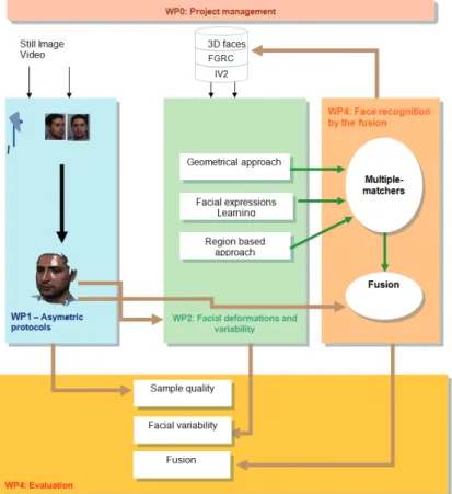
The present thesis was supported by the ANR under the project ANR-07-SESU-004. The project is known as Facial Analysis and Recognition Using 3D (FAR3D). The aim of the FAR3D project is to develop algorithms and techniques in 3D face recognition answering in particular the 3D challenges related to 3D acquisition, face expression variation and face recognition reliability/stability versus 3D face model quality (resolution and depth precision). Two face recognition scenarios will be studied within the project: on the one hand face recognition in symmetrical mode by comparing a probe 3D face model with the ones in the gallery, and on the other hand face recognition in asymmetrical mode by comparing an image or sequence of 2D facial images (probe) with the gallery ones. Figure 1.1 illustrates the bloc diagram of the project tasks, we are concerned by the geometric approach.The partners are Ecole Centrale de Lyon/LIRIS, Eurecom, THALES and USTL/LIFL which is the coordinator of the project.

1.1 Problematic and Motivation

The need for civil defense on the one hand and the fight against fraud, crime and terrorism on the other hand, make person’s identity verification an ultimate aim for computer vision researchers. Person’s identity can be checked in one of three ways: by something they have (e.g. an ID card); something they know (e.g. the answer to a security question); or

(17)

Chapter 1. Introduction

Figure 1.1: bloc diagram of the project tasks.

something they are (a biometric). Several special biometrics are suitable for differentiating persons from others. Biometrics such as faces, iris patterns, hand geometry, fingerprints, speech, retina, dynamic signature, and gait are among the most frequently used modalities. By human biometrics we mean the use of physiological characteristics, human body parts and their appearances, to pinpoint individual human beings in the course of daily activities. The appearances of body parts, especially in imaged data, have a large variability and are influenced by their shapes, colors, illumination environment, presence of other parts, and so on. Therefore, the biometrics researchers have focused on body parts and images that try to minimize this variability within class (subjects) and maximize it across classes. The use of shapes of facial surfaces (or 3D faces) is an important example of this idea. Actually, face recognition has many benefits over other biometric technologies due to the

(18)

1.1. Problematic and Motivation

natural, non-intrusive, and high throughput nature of face data acquisition. Thus, the techniques for face recognition have received a growing attention within the computer vision community over the past three decades. Since 2D (visible light) images of faces are greatly susceptible to variations in the imaging environments (camera pose, illumination patterns, etc), the researchers have argued for the need to use 3D face data, typically collected by laser scanners, for studying shapes of peoples’ faces and using this shape analysis for biometrics. The output from laser scanners are minimally dependent on the external environmental factors and provide faithful measurements of shapes facial surfaces. It’s the case the only remaining variability that is manifested within the same class, i.e. within the measurements of the same person, is the one introduced by changes in facial expressions, self occlusion (due to pose variation) and aging. Facial expressions, such as smile, serious, fear, and anger, are prime indicators of the emotional state of a person and, thus, are important in estimating mood of a person, for example in developing intelligent ambient systems, but may have a lesser role in biometric applications. In fact, change in facial expressions changes the shapes of facial surfaces to some extent and introduce a nuisance variability that has to be accounted for in shape-based 3D face recognition. We argue that the variability introduced by facial expressions has become one of the most important issue in 3D face recognition. The other important issue is related to data collection and imperfections introduced in that process. It is difficult to obtain a pristine, continuous facial surface, or a mesh representing such a surface, with the current laser technology. One typically gets holes in the scanned data in locations of eyes, lips, and outside regions. For instance, scans of people with open mouths result in holes in the mouth region. Moreover, when the subject is non cooperative and the acquisition phase is unconstrained, one gets variation in pose and unforeseen extraneous occlusions. Many studies treated pose and expression variation but few ones tried to focus on solving the problem of occlusion even if a face can easily be partially hidden by objects like glasses, hats, scarves or a hand, hair and beard. Occluded parts represent wrong information which can degrade recognition accuracy, so how to locate and remove occlusion on face quickly and automatically is a challenging task.

In the biometrics literature, recognition is a general term which includes identification and verification. However, recognition mostly refers to identification in many papers, and

(19)

authentication is used instead of verification.

One application of the verification task is access control where an authorized individual is seeking access to a secure facility and presents to the system his or her identity. Here, a one-to-one matching is performed : the 3D image for this individual is acquired, preprocessed and finally compared to an enrollment acquisition already incorporated in the system database. If the similarity is greater than a defined threshold the subject is granted access, otherwise access is denied. The identification scenario consists on determining identity of an authorized user in a database of many individuals. As far as verification scenario is concerned, it is important to examine the probability of correct verification as a function of the false acceptance rate (or Imposter access). This is often shown with a Receiver Operating Characteristic (ROC) curve that graphs the probability of correct verification versus the false acceptance rate. In the identification scenario, however, the results for facial identification are often displayed using a Cumulative Match Characteristic (CMC) curve. This curve displays the cumulative identification rates as a function of the rank distribution. This provides an indication of how close one may be to getting the correct match if the rank-one match was incorrect

1.2 Goals and contributions

In this thesis, we investigate shape analysis for 3D facial surfaces comparison, averaging and restoration. The contributions can be grouped according to the following categories:

• Riemannian Analysis of 3D Nose Shape For Partial Human Biometrics. The nose region is observed as the most stable region in the face during expression variations. We propose to study the contribution of this biometric in person identification. The main tool presented is the construction of geodesic paths between two arbitrary nasal surfaces. The length of a geodesic between any two nasal surfaces is computed as the geodesic length between a set of their nasal curves. In particular, we present results for computing geodesics, computing statistical means and stochastic clustering to perform hierarchical clustering. We demonstrate these ideas in two application contexts : the authentication and the identification biometric scenarios using nasal shapes on a large

(20)

1.2. Goals and contributions

dataset involving 2000 scans, and hierarchical organization of noses gallery to allow efficient searches.

• Pose and Expression-Robust 3D Face Recognition Using Elastic Radial Curves. Our contribution here is an extension of the previous elastic shape analysis framework [JKSJ07] of opened curves to surfaces which is able to model facial deformations due to expressions, even when the mouth is open. The key idea here is the representation of a face by its radial curves, and the comparisons of those radial curves using the elastic shape analysis. We demonstrate the effectiveness of our approach by comparing to the state of the art results. However, unlike previous works dealing with large facial expressions, especially when the mouth is open which require lips detection, our approach mitigates this problem without any lip detection. In [DBADS10], we test this algorithm on FRGC v2 dataset and organize hierarchically the face gallery to allow efficient searches. We illustrate this geometric analysis of 3D facial shapes in presence of both facial expressions and pose variations. We report results on GAVAB dataset and our result outperforms previous works on that dataset. We present the results of our approach in 3D face recognition designed to handle facial expression variations, pose variations and missing data between gallery and probe images. The method has several benefits that make it suited for 3D face recognition and retrieval in a large dataset. Firstly, to handle a pose variation and missing data, we propose a local representation by using a curve representation of 3D face and a quality filter of a curves. Secondly, to handle variations in facial expressions, we propose an elastic shape analysis of 3D face. Lastly, to accelerate the running time of recognition algorithm we propose hierarchical organization of the gallery to allow for efficient retrieval. Experiments that are performed on the FRGCv2 and GavabDB databases and within the SHREC’10 contest show high effectiveness also in the presence of large facial expressions, pose variations and missing data. For the identification experiment, we achieve the second best recognition rate of 97.7% on FRGCv2 and the best rank (96.99%) on GavabDB. The behavior of our algorithm in presence of different kind of quality degradation is analyzed through the next analysis. We simulate the presence of noise, missing data and decimation on a subset of FRGC v2 dataset, then we present

(21)

a comparative study of the results of our algorithm performed on these data.

• 3D face shape restoration: Application to 3D face recognition in presence of occlusions. Our contribution here is a novel framework for 3D face shape restoration.

3D face recognition in presence of missing data : the surface is first represented by radial curves (emanating from the nose tip for the example of the 3D face). Then a statistical computation on non linear manifold are proposed to built eigen-curves basis. Hence, the missing part of the curve can be restored by projecting the existing part of it on the base.

1.3 Organization of the thesis

This thesis is organized as follows: in chapter two we lay out challenges and the state of the art on 3D face recognition task. In chapter three, we study the contribution of the nose region, seen as the most stable region in the face under expression variations. Chapter four describes our approach for 3D face recognition. The same framework used for recognition is used to calculate statistics in chapter five. Finally we present concluding remarks and some perspectives of the current work in the last chapter.

(22)

Chapter 2

State-of-the-art on 3D face

recognition

2.1 Introduction

The full 3D model of a human head can be acquired from multi-view stereo systems during the scanning process. However, multi-view are not practical for recognition scenarios. Therefore, static 3D sensors such as laser scanners or structured light based stereo systems produce the so-called 2.5D image (depth map or range image). 2.5D surface is usually defined as having at most one z-depth measurement from a given (x,y) coordinate. It is possible to generate full 3D face models by combining several 2.5D images. In the 3D face recognition literature, the term 3D is commonly used to denote 2.5D data. In terms of a modality for face imaging, a major advantage of 3D scans over 2D color imaging is that variations in illumination, pose and scaling have less influence on the 3D scans. Actually, three dimensional facial geometry represents the geometric structure of the face rather than its appearance influenced by environmental factors. For instance, 3D data is insensitive to illumination, head pose [BCF06b], and cosmetic [MS01]. Therefore, 3D face acquisition requires more sophisticated sensor than 2D one. The rest of this chapter in organized as follow. In section 2, we describe the acquisition process and survey available 3D face databases. Section 3 enumerates and describes the representations of a 3D face model. In

(23)

Chapter 2. State-of-the-art on 3D face recognition

section 4, we summarize the challenges of 3D face recognition. Section 5 gives necessary elements to describe the geometry of a 3D face. Sections 6, 7 and 8 describe the previous approaches. In section 9 we discuss the previous approaches and we finally give concluding remarks in section 10.

2.2 3D Face acquisition and available databases

Many technical solutions have been proposed for the acquisition of 3D geometry from human face. Even if Computer Vision practitioners have made a significant effort to develop less expensive alternative techniques based on passive sensors, most 3D face databases are collected by active sensors. Active techniques are based on lighting up the 3D face. Most of laser scanners use an optical camera and laser rays to measure by triangulation the distance to sample target points on the faces’ boundary to produce depth images. Depth images are 2D views of the face accompanied with the depth information (the distance from the face to the scanner) for each pixel. Laser-based sensors are able to produce a dense and precise reconstruction in about 0.5s for fast mode and 2.5s for high resolution mode. During acquisition, the subject should make no movement. However, they generate some noise and missing data due to laser absorption by dark area and self-occlusion as illustrated in Figure 2.6.b. Laser sensors are expensive as they need rotating mirrors and cylindrical lens to generate a plan of laser and scan the face. Figure 2.1 illustrates the output of the scanner as depth and color channels. The range and color image are illustrated at top row respectively by Figure 2.1.a and Figure 2.1.b. The 3D mesh is illustrated at bottom row in Figure 2.1.c, Figure 2.1.d shows the texture mapped on it.

Most popular 3D face datasets were collected using laser-based sensors. FRGCv1 and FRGCv2 were collected by researchers of the University of Notre Dame and contain 948 3D images for training (FRGCv1) and 4007 3D face for testing (FRGCv2) of 466 different persons belonging to different sex, different races and different ages [PFS+05]. We illustrate an example of faces from this database in Figure 2.2, left image illustrates the 3D data and right image illustrates the color image mapped on the 3D one.

(24)

2.2. 3D Face acquisition and available databases

(a) Range image

(b) Texture image

(d) Textured 3D model

(c) 3D model

Figure 2.1: Output of the 3D sensor: range and color image at top row and 3D mesh with and without color mapped on in bottom row.

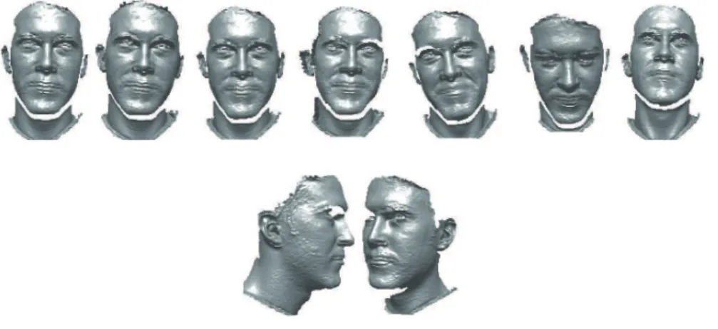
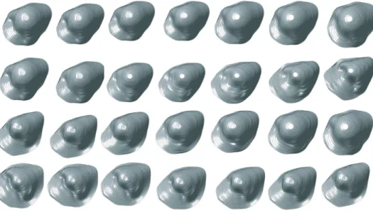
The GavabDB consists of Minolta Vi-700 laser range scans from 61 different subjects. The subjects, of which 45 are male and 16 are female, are all Caucasian. Each subject was scanned 9 times for different poses and expressions, namely six neutral expression scans and three scans with an expression. The neutral scans include two different frontal scans, one scan while looking up (+35 degree), one scan while looking down (-35 degree), one scan from the right side (+90 degree), and one from the left side (-90 degree). The expression scans include one with a smile, one with a pronounced laugh, and an arbitrary expression freely chosen by the subject [MS04]. Figure 2.3 shows some examples of faces in this dataset.

(25)

Figure 2.2: Example of face from FRGCv2 face. 3D data is shown at top and the texture is mapped on it at the bottom.

(a) (b) (c) (d) (e) (f ) (g)

(i) (h)

Figure 2.3: Examples of all 3D scans of the same subject from GAVAB dataset. GavabDB is used by many researchers to compare their methods. However, the commonly used Benchmark for the task of 3D face recognition is FRGC. New challenges such as face occlusion and typical expression classification are not considered by these datasets. The typical expressions classification is not the main task in this manuscript, however, the face occlusion is a new challenge on 3D face recognition. BOSPHORUS database [SAD+08] is the suitable 3D face database for that task; Actually, it contains facial models of 60 men and 45 women, 105 subjects in total, in various poses, expressions and in presence of occlusions (eyeglasses, hand, hair). The majority of the subjects are aged between 25 and 35. The number of total face scans is 4652, where for every subject 54 scans are available,

(26)

2.3. 3D face representations

but 34 of them have 31 scans. For each subject, four occluded scans were gathered. These occlusion are i) mouth occlusion by hand, ii) eyeglasses, iii) occlusion of face with hair, and iv) occlusion of left eye and forehead regions by hands. Figure 5.18 shows sample images from the Bosphorus 3D database illustrating expression variations and typical occlusions.

Figure 2.4: Examples of faces from the Bosphorus and illustration of the problems of incomplete data (due to the pose or occlusion) and deformations of the face (due to expressions).

We present in Table 2.1 a summary of the most known and available 3D face datasets and their characteristics.

Table 2.1: Popular 3D face datasets and their different characteristics.

Sensor used Number of subjects Total scans Expressions Missing data Occlusion

FRGCv1 Laser sensor 275 948 No No No

FRGCv2 Laser sensor 466 4007 Yes No No

GavabDB Laser sensor 61 549 Yes Yes No

BosphorusDB Structured light 105 4652 Yes Yes Yes

2.3 3D face representations

Despite all physical objects that surround us are continuous, digital computers can only work with discrete data. Therefore, surfaces are usually approximated using discrete representations. The most noticeable exception being represented by NURBS modeling. As far as 3D face is concerned, the output of 3D sensors is a range image accompanied with a color image. This specific representation is illustrated in Figure 2.1.a and Figure

(27)

2.1.b. The range image has the same resolution as the color one. The values of color level are replaced in that case by the depth value (distance to the sensor). Therefore, the neighborhood of points in 3D in known and the 3D model (illustrated in Figure 2.1.c can be constructed).

Cloud of points 3D mesh

Zoom in

(a) 3D face model

Range image

(b) 3D face representa!ons

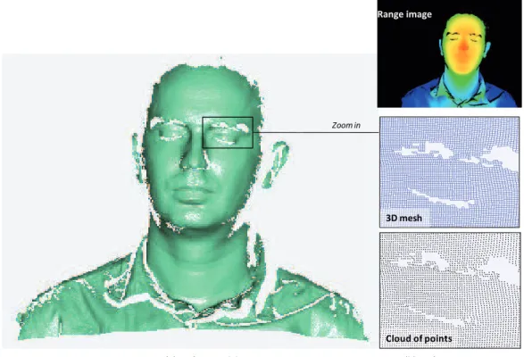
Figure 2.5: 3D face model and different representations: point cloud and 3D mesh. Figure 2.5.a illustrates the 3D model reconstructed from range image. The different representation of the 3D face are illustrated in Figure 2.5.b. The top image illustrates the range image, the middle one illustrates a zoom on the resulting mesh and the bottom image illustrates a zoom on the cloud of points. The representation of the 3D face by range image allows the use of 2D image processing algorithms. The point cloud representation is used by several algorithms which do not need to know the neighborhood of points.

A surface mesh representation is given by the definition of an arbitrary number of sample points p of coordinates (x, y, z) lying on the surface. Then the surface is locally

(28)

2.4. Challenges of 3D face recognition

approximated by polygon primitives (especially triangles) which connect the sample points into a graph structure, denoted as a polygon mesh M. The polygon primitives are denoted as faces f , the segments of faces as edges e and the extremities as vertices v (one vertex per sample point p):

M = {V, E, F }, F = {f1, f2, ..., fN}, E = {e1, e2, ..., eN} and V = {v1, v2, ..., vN}.

The automatic reconstruction of the mesh surface from point sets is an active research topic which is far beyond the scope of this manuscript. We defer the reader to (MM99) for a detailed survey and to (KBH06, SLSL06, BHGS06) for recent automatic techniques. In practice, interactive techniques based on the canonical Delaunay triangulation are mostly employed and can be considered as part of the acquisition operation.

2.4 Challenges of 3D face recognition

When acquired in non-controlled conditions, scan data often suffer from the problem of missing parts due to self-occlusions or laser-absorption by dark areas. Actually, the 3D face needs more than one scan to be fully acquired. Especially when the pose is not frontal as illustrated in Figure 2.6.b, the resulting scan is said 2.5D and not full 3D. However, this 2.5D scan is roughly approximated by 3D scan by 3D face recognition community researchers. Moreover, bottom row in Figure 2.6.b illustrates that dark area (hair or eyebrows) absorb the laser and generate missing data in the 3D mesh as illustrated at the top row of the same figure.

Additionally, variations in face data due to facial expressions cause deformations in the 3D mesh. Figure 2.6.a illustrates expressive faces at the bottom row (as 3D textured mesh). The top row illustrates the resulting 3D mesh with deformations.

Any 3D face recognition approach should successfully match face scans in presence of expression-based deformations and/or missing data (as illustrated respectively in Figure 2.6.a and Figure 2.6.b) to good quality, neutral, frontal 3D model. We note that generally the enrolled face scans are collected in controlled conditions and exhibit good data quality. Past literature has tackled this fundamental issue with a varying degree of success as described in the survey paper [BCF06a].

(29)

(a)

(b)

Figure 2.6: Deformations under facial expressions (a). Missing data due to self occlusion (b).

We start with modeling the geometry of human faces, next we will present most recent and elaborated approaches for that task.

2.5 Elements on geometry of facial surfaces

From geometric point view, a human facial surface can be modeled as a two-dimensional manifold, denoted by S. Roughly speaking, manifolds with finite dimension can be defined as topological spaces having locally similar structures to Rn. Every element of a manifold should belong to neighborhood which is homomorphic to a neighborhood in Rn_{. In topology,}

a diffeomorphism is an isomorphism in the category of smooth manifolds. It is an invertible function that maps one differentiable manifold to another, such that both the function and its inverse are smooth.. Therefore, the parametrized facial surface can be seen a differential application from an open set of R2 to an open set of R3. The parametrized surface is said regular if for each point (u, v) ∈ U , the vectors ∂X_∂u(u, v) and ∂X_∂v(u, v) are linearly

(30)

2.5. Elements on geometry of facial surfaces

independent. In that case, the derivatives ∂X_∂v(u, v) and ∂X_∂u(u, v) constitute a local non-orthogonal coordinate system on S, and span an affine subspace of R3 called the tangent space and denoted by Tx(S) for every x ∈ S. The restriction of the euclidean inner product

to the tangent space Tx(S) is called first fundamental form. This metric is intrinsic to

the manifold S and allows to perform local measures independently of the coordinates of the embedding space[Kre91]. Using this metric, let d, the surface will be considered as metric space (S, d) or Riemannian manifold. In order to define an intrinsic distance, let x, y ∈ S be two points on the surface and let c : [0, 1] → S be a smooth curve in arc length parametrization connecting x and y on S. The length of c is defined by:

l[c] = Z 1

0

kdc(t)

dt k dt. (2.5.1)

Then the intrinsic distance on S between the two points is given by

d(x, y) = inf

c l[c]. (2.5.2)

The paths of minimum length is obtained by the minima of the function l[c] and called minimal geodesics, and the resulting distance d(x, y) is called geodesic distance. Figure 2.7 illustrates the euclidean and geodesic distances between two points on the face surface.

Euclidean distance Geodesic distance

Figure 2.7: Euclidean path (in red) and geodesic one (in blue) on facial surface There are two main algorithms in a 3D mesh processing literature that can be applied on the facial surface mesh to calculate the geodesic distance between any pair of points on it: the Dijkstra algorithm and the Fast marching algorithm. These are briefly described in

(31)

the following.

2.5.1 Algorithms for geodesic computation on surfaces

• Dijkstra algorithm: we start our discussion by considering the surface mesh as a graph, then we will extend it to triangular meshes. For a given source vertex (node) in the graph, the Dijkstra algorithm [Dij59] finds the path with lowest cost (i.e. the shortest path) between that vertex and every other vertex. It can also be used for finding costs of shortest paths from a single vertex to a single destination vertex by stopping the algorithm once the shortest path to the destination vertex has been determined. In our case, the edge path costs represent the length of the edge, Dijkstra’s algorithm can be used to find the shortest route between two given vertices in the surface. • Fast marching algorithm

The fast marching algorithm [Set96] is characterized by flame propagation. The typical illustration of flame propagation in a forest helps to understand how fast marching works. Trees reached by the fire are consumed so the fire never propagates backward. To evacuate people, the firemen try to record front position at different positions in time. Hence, they can predict when the fire arrives to unburnt regions of the forest and order evacuation of people. The time of arrival of the fire front to a point in the forest is related to the shortest distance from that point to the source of the fire.

Fast marching algorithm has the ability to find paths passing ’between’ the graph edges and this can be of interest in case of low resolution meshes. In case of facial surface acquired with laser sensors, the resolution is quite hight and Graph-based algorithm, such as Dijkstra’s, can be considered as one of best choices for finding shortest paths lengths.

2.5.2 Facial expressions modeling

Let (S1, g) and (S2, h) be two facial surfaces modeled as Riemannian manifolds. Particularly,

(32)

2.5. Elements on geometry of facial surfaces

metric dS2 on S2. The two faces belong to the same person (the author) but S1 is a neutral

face whereas S2 is an expressive one. Let f : S1 → S2 be a diffeomorphism modeling the

expression (see Figure 2.8).

The diffeomorphism between two topological spaces is a continuous bijection, and the inverse application is continuous. Roughly speaking, a topological space is a geometric object, and the diffeomorphism is a continuous stretching and bending of the object into a new shape. Thus, a neutral face and an expressive one are diffeomorphic to each other. Notice that the holes (like open mouth) should be filled, otherwise this assumption is false. Some authors [BBK05] approximate this diffeomorphism by an isometry. In other words, they assume that f preserves the geodesic distance between every pair of points, that is,

dS1(x, y) = dS2(f (x), f (y)), ∀x, y ∈ S1. (2.5.3)

Neutral face _{Expressive face}

f

Figure 2.8: Points correspondence (neutral face at left and expressive face at the right) Several approaches adopt this assumption and used geodesic distance on the facial surface to design expression-invariant approaches.

(33)

2.6 Geodesic-based approaches

In [BBK05], the authors presented an experimental validation of the isometric model. They placed 133 markers on a face and tracked the change of both euclidean and geodesic distances under facial expressions. The distribution of the absolute change of geodesic distances was closer to zero than the distribution of the change of euclidean distance. Therefore, the authors assumed that the change of geodesic distance is insignificant and conclude that geodesic distance remains unchanged under facial expression. Under this assumption, in [BBK05], they represent 3d faces as canonical forms. Canonical surfaces were obtained from face surfaces by warping according to a topology preserving transformation. Finally face models were represented with the geometric moments up to the fifth order computed for the 3D face canonical forms. However, while the effect of expressions was attenuated, a similar attenuation also occurred for discriminating features such as eye sockets and nose. This approach was improved in [BBK06] where the authors handled the challenge of missing parts. They embed the probe facial surface into that of the gallery. Faces belonging to the same subject are nearly isometric and thus result in low embedding error, whereas different subjects are expected to have different intrinsic geometry, and thus produce higher embedding error. The open mouth corrupts the isometric model. This problem was handled later by the authors in [BBK07] by using geodesic mask excluding the mouth region. The authors first detected and removed the lips, then the computation of geodesic distance geodesics is calculated on surface in presence of a hole corresponding to the removed part. This is done while avoiding passing in mouth area.

The assumption of the isometric model motivated several authors to use geodesic distance on facial surface. In [SSDK09], the geodesic distance to the tip of the nose were used as surface distance function. Differential geometry was used to compare 3D level curves of the surface distance function. This approach was an improvement of an earlier work of the authors [SSD06], were they used the level curves of the height function to define facial curves. The use of geodesic distance in [SSDK09] allows this approach to handle facial expressions. However, the open mouth corrupts the shape of some level curves and this parametrization did not address this problem, and the experiments were restricted to

(34)

2.7. Deformable template-based approaches

a small subset of FRGCv2 database.

A similar geodesic polar parametrization of the face surface was proposed in [MMS07], but rather than studying the shape of curves, they studied local geometric attributes under this polar parameterization. To handle data with open mouths, they modified their geodesic polar parametrization by disconnecting the lips. Therefore, their approach required lips detection, as was the case in [BBK07].

In [BBP10], the authors used the geodesic distance on the face to extract iso-geodesic facial stripes. Equal-width iso-geodesic facial stripes were used as nodes of the graph and edges between nodes were labeled with descriptors, referred to as 3D Weighted Walkthroughs (3DWWs), that captured the mutual relative spatial displacement between all the pairs of points of the corresponding stripes. Face partitioning into iso-geodesic stripes and 3DWWs together provided an approximate representation of local morphology of faces that exhibits smooth variations for changes induced by facial expressions.

A common limitation of the previously described approaches is that they assume that the facial shape deforms isometrically, i.e. the surface distances between points are preserved, which is not valid in the case of large expressions. Actually, the movement of mimic muscles can stretch and/or shrink the face surface and not only bending it. The deformation caused by the expression in Figure 2.8 illustrates that it is not isometric. This will be discussed in more details in chapter 4.

2.7 Deformable template-based approaches

In recent years there has been focus on deforming surfaces, one into another, under a chosen criterion. Grenander’s deformable template theory [Gre93] has been successfully applied to studying shapes of anatomical parts using medical images [MY01, GM98]. The set of non-rigid deformations can be subdivided into linear and nonlinear deformations. Nonlinear deformations imply local stretching, compression, and bending of surfaces to match each

(35)

other, and are also referred to as elastic deformations. Earlier attempts at elastic matching utilized graphs based on texture images of faces [KTP00].

Kakadiaris et al. [KPT+_{07] utilize an annotated face model to study geometrical variability}

across faces. The annotated face model is deformed elastically to fit each face thus allowing the annotation of its different anatomical areas such as the nose, eyes and mouth.

Points of an annotated 3D face reference model were shifted according to elastic constraints so as to match the corresponding points of 3D target models in a gallery. Similar morphing was performed for each query face. Then, face matching was performed by comparing the wavelet coefficients of the deformation images obtained from morphing. This approach is full automatic. Similar approaches were based on manually annotated model [MMS08, LJ06, LJ08].

In [LJ08], the authors presented an approach that is robust to self-occlusions (due to huge pose variations) and expressions. 3D deformations learned from a small control group was transferred to the 3D models with neutral expression in the gallery. The corresponding deformation was synthesized in the 3D neutral model to generate a deformed template. The matching was performed by fitting the deformable model to a given test scan, which was formulated as a minimization of a cost function.

In [tHV10], the authors propose a multi-resolution approach to semi-automatically build seven morphable expression models, and one morphable identity model from scratch. The proposed algorithm automatically selects the proper pose, identity, and expression such that the final model instance accurately fits the 3D face scan.

A strong limitation of these approaches is that the fiducial landmarks needed during expression learning have to be extracted manually for some approaches. They are usually semi-automatic and rarely full automatic.

(36)

2.8. Local regions/ features approaches

2.8 Local regions/ features approaches

A different way proposed in the literature to handle expression variations is to match parts or regions of faces rather than the whole faces. Several notable local techniques were proposed in [Gor92, MSVD05] where the authors employed surface areas, curvatures around facial landmarks, distances and angles between them with a nearest neighbour classifier. In [LSY+_{05], based on ratios of distances and angles between eight fiducial}

points, the technique used a support vector machine classifier. Euclidean/geodesic distances between anthropometric fiducial points were employed as features in [GAMB07] along with linear discriminant analysis classifiers. However, a successful automated detection of fiducial points is critical here.

In [MFA08, MAM09], the authors presented low-level geometric features-based and reported results on neutral faces but the performance decreases when expressions variations were introduced. Using similar features, the authors in [LJZ09] proposed to design a feature pooling and ranking scheme in order to collect various types of low-level geometric features, such as curvatures, and rank them according to their sensitivities to facial expressions. They applied sparse representations to the collected low-level features and achieved good results on a challenging dataset (GavabDB [MS04]). This approach, however, required a training step.

Along similar lines, in [WLT10], a signed shape difference map (SSDM) was computed between two aligned 3D faces as an intermediate representation for the shape comparison. Based on the SSDMs, three kinds of features were used to encode both the local similarity and the change characteristics between facial shapes. The most discriminative local features were selected optimally by boosting and trained as weak classifiers for assembling three collective strong classifiers. The individual features were of the type: Haar-like, Gabor, and Local Binary Pattern (LBP).

In [MR10], the authors used 3D Fisherface region ensemble approach. After faces registration using ICP algorithm, the Fisherface approach seeks to generate a scatter matrix for improved classification by maximizing the ratio of the between scatter and within

(37)

scatter. Twenty-two regions were used as input for 3D Fisherface. In order to select most discriminative regions, Sequential Forward Search [STG08] was used.

In [HZA+10, HAWC11, HOA+11], the authors propose to use the Multi-scale LBP as a new representation for 3D face jointly to shape index. SIFT-based local features are then extracted. The matching involves also holistic constraint of facial component and configuration.

In [CMCS06], the Log-Gabor templates were used to exploit the multitude of information available in human faces to construct multiple observations of a subject which were classified independently and combined with score fusion. Gabor features were recently used in [MMJ+10] on automatically detected fiducial points.

In [CBF06, MBO07] the focus was on matching nose regions albeit using ICP. To avoid passing over deformable parts of the face encompassing discriminative information, the authors in [FBF08] proposed to use a set of 38 face regions that densely cover the face and fused the scores and decisions after performing ICP on each region.

In [QSBS10], the circular and elliptical areas around the nose were used together with forehead and the entire face region for authentication. Surface interpenetration measure (SIM) were used for the matching. Taking advantage of invariant face regions, an Simulated annealing approach was used to handle expressions.

In [AGD+08], the authors proposed to use the Average Region Models (ARMs) locally to handle the missing data and the expression-inducted deformation challenges. They manually divided the facial area into several meaningful components and registration of faces was carried out by separate dense alignments to relative ARMs. A strong limitation of this approach is the need for manual segmentation.

2.9 Discussion

The previous description of state of the art illustrates that recent research on 3D face recognition can be categorized into three classes. The geodesic-distance based approaches

(38)

2.10. Conclusion

are based on intrinsic distance and have the advantage to be independent of the embedding of the surface. In term of robustness to different challenges, these approaches are sensitive to noise, missing data and large expressions involving stretching and/or shrinking of the face and thus geodesic distance variation. These deformations due to large expressions are handled by deformable template-based approaches. These approaches are usually based on an annotated face model which deforms based on deformation of the landmarks. In term of accuracy, local approaches have shown best performances in general. Local approaches are usually based on matching stable regions together and reduce the effect of matching non stable regions.

In this thesis, we present a unified Riemannian framework that provides optimal matching, comparisons and deformations of faces using a single elastic metric. The proposed framework handles large expressions as well as missing parts due to large pose variation and occlusions. The first tool proposed in this thesis concerns partial biometric. That is, the construction of geodesic paths between arbitrary two nasal surfaces. The length of a geodesic between any two nasal surfaces is computed as the geodesic length between a set of their nasal curves. Facial surfaces are represented by collections of radial curves which allows local matching in order to handle pose variation, expressions and occlusion challenges. In addition, using the same framework, we are able to compute some statistics on 3D facial surfaces. This allows an hierarchical organization for efficient shape retrieval and missing parts restoration.

2.10 Conclusion

In this chapter, we first presented the 3D face acquisition process, the different repre-sentations of the 3D facial surface and the available benchmark datasets. The different representation of 3D facial surface. This allows the lay out of different challenges in 3D face recognition task. Second we present the geometric modeling of the 3D face, we present an early observation showing that the deformations of the face resulting from facial expressions can be modeled as isometries such that the intrinsic geometric properties of the facial surface, like geodesic distance, are expression-invariant. We presented the past approaches who were based on that assumption, even it is not valid in case of elastic deformation.

(39)

Then, we presented approaches based on face deformation. Finally we present the third kind of 3D face recognition approaches, based on local regions/features matching. At the end of the chapter, we discussed the presented approaches with their robustness to different challenges. The limitations of previous 3D face recognition approaches motivate further researches on several tasks as missing parts and non isometric deformations. We introduce our approach in this context.

(40)

Chapter 3

3D nose shapes analysis for partial

biometrics

3.1 Introduction

In order to handle shape variability due to facial expressions and presence of holes in mouth, we advocate the use of nose region for biometric analysis. At the outset the shape of the nose seems like a bad choice of feature for biometrics. The shapes of noses seem very similar to a human observer but we will support this choice using real data and automated techniques for shape analysis. We do not assert that this framework will be sufficient for identifying human subjects across a vast population, but we argue for its role in shortlisting possible hypotheses so that a reduced hypothesis set can be evaluated using a more elaborate, multi-modal biometric system.

Why do we expect that shapes of facial curves are central to analyzing the shapes of facial surfaces? There is plenty of psychological evidence that certain facial parts, especially those around nose, lips and other prominent parts, can capture the essential features of a face. Our experiments support this idea in a mathematical way. We have computed geodesic distances between corresponding facial curves of different faces – same people different facial expressions and different people altogether. We have found that the distances are typically smaller for faces of the same people, despite different expressions, when compared to the

(41)

Chapter 3. 3D nose shapes analysis for partial biometrics

distances between facial curves of different people.

The stability of nose data collection, the efficiency of nasal shape analysis, and the invariance of nasal shape to changes in facial expressions make it an important region of the face.

To resume, the nose region has certain advantages over the face, for example :

1. The robustness to facial expressions of nose region. Indeed, its shape undergone less variation compared with other regions like mouth, eyes, etc..under facial expressions. 2. The nose region is immune to missing data (holes) due to the open mouth in case of

frontal poses.

3. The pre-processing speed to extract features and informative region. 4. The efficiency of nasal shape analysis.

Our approach for analyzing shapes of the nasal surface is to represent such a surface by a dense collection of curves. These curves are defined such that they do not depend on the pose of the original face and have been used for full face recognition earlier. In the experimental results presented previously [ADB+09], we worked only with limited facial expressions, i.e. large facial expressions involving open mouths were avoided. Also, it was assumed that the holes are small enough to be filled by simple linear interpolations. The Figure 3.1 shows an example of extraction of facial curves for a 3D scan with large expression. Figure 3.2 illustrates histograms of distances for some level curves of geodesic distance to the tip of the nose. The three top histograms correspond to the distributions of distances calculated between curves lying on nasal region of the same person with different sessions. The distances have small values in contrast with distances shown in the down three histograms. The curves concerned in these histograms lie outside the nose region. As illustrated in the figure, the values of distances are quite high compared to the distances lying on the nose region. This experience advocates our assumption that a curve from the nose region is stable and captures the underlying true shape, while a curve from outside the nose region is significantly distorted due to the open mouth. If such a distorted curve is used to study the shape of the underlying facial surface, it will be difficult to distinguish people from one another.

(42)

3.1. Introduction

Figure 3.1: An illustration of challenges in facial shape in presence of large expressions. The level curves of geodesic distance to the nose tip lying in regions outside the nose are significantly distorted while the curves in nose region remain stable.

(43)

Our framework for quantifying shape differences between 3D surfaces is based on accumulating shape differences between the curves representing the two surfaces. This difference between shapes of curves, in turn, is computed by constructing geodesic paths under the elastic metric on a Riemannian space of closed curves in R3. On one hand these distances are useful in quantifying shape differences between objects, for example faces or parts of faces belonging to different people. On the other hand, they are also useful in studying variability in shapes of curves resulting from changes in facial expressions. For instance, we have computed distances between level curves on faces of sample people but under different expressions. Two types of curves were used in this experiment: the curves that lie in the nose region and the curves that lie outside the nose region.

0.1 0.2 0.3 0.4 0.5 0.6 0.7 0 0.5 1 1.5 2 2.5 3 Distance 0.1 0.2 0.3 0.4 0.5 0.6 0.7 0 0.5 1 1.5 2 2.5 3 3.5 4 0.1 0.2 0.3 0.4 0.5 0.6 0.7 0 0.5 1 1.5 2 2.5 3 0.1 0.2 0.3 0.4 0.5 0.6 0.7 0 0.5 1 1.5 2 2.5 3 0 0.1 0.2 0.3 0.4 0.5 0.6 0.7 0 0.5 1 1.5 2 2.5 3 3.5 4 4.5 5 0.1 0.2 0.3 0.4 0.5 0.6 0.7 0 0.5 1 1.5 2 2.5 3 Distance Distance

Distance Distance Distance

Level 6 Level 8 Level 18

Level 40 Level 44 Level 48

Figure 3.2: Histograms of distances (for some level curves) between different sessions of the same person

The rest of this chapter is organized as follows, section 2 gives a brief description of the preprocessing step. In section 3, we explain the differential-geometric framework of curves

(44)

3.2. Automatic 3D scan preprocessing

and its extension to 3D surfaces that we used to analyze 3D shapes of nose region. Finally, in section 4, we show the experimental protocol, some preliminary results on a subset of FRGC v2 database containing expressive faces and large scale results.

3.2 Automatic 3D scan preprocessing

In order to assess the recognition performance of the proposed framework, we use 3D models of FRGCv2 dataset. This benchmark database contains sessions with both neutral and non-neutral expressions. Moreover, the laser-based 3D scanner used in the acquisition process introduces noise in the data. In fact, some of 3D face scans suffer from missing data (holes), spikes, artifacts specially in teeth region, occlusions caused by the hair, etc.

We focus in this work on designing a complete solution for 3D face analysis and recognition using only the nose region. For that purpose, it is crucial to begin by de-noising the data by removing spikes, filling holes and extract only the useful part of face and then nose from 3D scan. Figure 3.3 shows different steps of our preprocessing solution to overcome these problems. Starting from an original range image of a face, we firstly apply a 2D median filter in order to remove spikes while preserving edges. Secondly, using a smooth interpolation, we fill holes by adding points in parts where the laser has been completely absorbed (e.g. eyes, eyebrows and open mouth). This is done based on cubic interpolation (splines). On the triangular mesh, we apply the procedure shown in Figure 3.4 to localize the nose tip, necessary for cropping the useful region of the face and nose region segmentation. For this purpose, a sphere function having center the nose tip and radius R = 100mm is constructed and the part inside the sphere is kept. Finally, a collection of geodesic level curves are extracted by locating iso-geodesic points from the reference vertex (nose tip) using the Dijkstra algorithm [Dij59]. In order to segment nose region, we consider the N first level curves (N = 10):

• Nose tip detection We are able to automatically detect the tip of the nose when the 3D face is frontal. This is verified in 3D models of FRGCv2 dataset. Through the center of the mass of the face, a first transverse plane (parallel to x-z plane) slices the facial surface. The intersection of the plane and the surface results in a horizontal

(45)

Chapter 3. 3D nose shapes analysis for partial biometrics Removing spikes (Median filter) - Filling holes (Interpolation) - Mesh generation (Delaunay)

- Nose tip detection Face cropping - Face smoothing - Geodesic level

curves extraction - nose segmentation Original range image

FileID = 02463d546

Final 3D face model

Number of cells: 40194 Number of points: 20669 Memory: 1.04 MB

Geodesic curves on nose region

Figure 3.3: Automatic FRGC data preprocessing and nose curves extraction. profile of the face. A second sagittal plane (parallel to y-z plane) passing through the maximum of the obtained horizontal profile, cuts the face on a vertical profile. The nose tip is located at the maximum of the middle part of this 2D curve as illustrated in Figure 3.4. This step is very important in our general framework as it is necessary to correctly crop faces and extract level curves from the surface.

• Level curves extraction Our facial shape analysis algorithm operates using 3D curves extracted by computing geodesic length function along the face. This choice is motivated by the robustness of this function to facial deformations as described in [BBK05]. In addition to its intrinsic invariance to rigid transformations such as rotations and translations, this distance better preserves the separations of facial features as compared to the Euclidean distance in R3.

Let S be a facial surface denoting a scanned face. Although in practice S is a triangulated mesh, start the discussion by assuming that it is a continuous surface. Let dist : S −→ R+ be a continuous geodesic map on S. Let cλ denote the level set of

(46)

3.2. Automatic 3D scan preprocessing Transverse slicing Triangulated 3D model Sagittal slicing Nose tip extraction Nose tip Horizontal profile Vertical profile

Figure 3.4: Automatic nose tip detection procedure.

dist, also called a facial curve, for the value λ ∈ dist(S), i.e. cλ= {p ∈ S|dist(P ) =

GD(r, p) = λ} ⊂ S where r denotes the reference point (in our case the nose tip) and GD(r, p) is the length of the shortest path from r to p on the mesh. We can reconstruct S from these level curves according to =[

λ

cλ.

• Nose region segmentation Detecting nose region is not easy in general. Fortu-nately, our approach deals with level curves and the nose tip is the reference point. So, it will be easy to delimit the nose region, in our case, by decreasing of value of λ and reconstruct the nose from level curves according to N = ∪λcλ, for the value

λ ∈ D(N ), i.e. cλ = {p ∈ N |D(P ) = GD(r, p) = λ} ⊂ N where N denotes the

nose region. The output of the preprocessing step is a nasal surface, as illustrated by Figure 3.5.

The preprocessing is one of the main issues in this such problems, so we have combined the preprocessing steps described above to develop an automatic algorithm. This algorithm

(47)

Figure 3.5: Examples of pre processed data: nose region with geodesic level curves

Table 3.1: Results of preprocessing procedure on FRGCv2 dataset. Original files Success pre-processing failed pre-processing Success Rates (%) Fall 2003 1893 1877 16 99.15 Spring 2004 2114 1994 20 98.99 FRGC v2 4007 3971 36 99.1

has successfully processed 3971 faces in FRGCv2, which means a success rate of 99.1% as described in the Table 3.1. This automatic preprocessing procedure failed for 16 faces taken in Fall 2003 and 20 faces taken in Spring 2004. Actually, it is the nose detection step that fails more than other steps. The main cause is the additive information which moves the mass center far from the face and the profiles extracted do no more match with the face profiles. For these faces, we have fixed manually the nose tip and so we have cleaned all the FRGC v2 faces, 99.1% automatically and 0.9% manually. The nose tip is considered correctly detected when the difference between the extracted coordinates of the nose tip against the coordinates provided with the dataset does not exceed 0.8 cm.

3.3 A Geometric Framework for nose shape analysis

As indicated earlier, our goal is to analyze shapes of nasal region surfaces using shapes of facial curves. In other words, we divide each surface into an indexed collection of simple, closed curves in R3 and the geometry of a surface is then studied using the geometries of the associated curves. Since these curves, previously called facial curves, have been defined as level curves of an intrinsic distance function on the surface, their geometries in turn

Statistical Computing On Manifolds for 3D Face Analysis and Recognition

HAL Id: tel-00728009

https://tel.archives-ouvertes.fr/tel-00728009

Statistical Computing On Manifolds for 3D Face

Analysis and Recognition

Hassen Drira

To cite this version:

Hassen DRIRA

Statistical Computing On Manifolds for 3D Face Analysis and

Recognition

Acknowledgements

Table of contents

List of figures

Chapter 1

Introduction

1.1

Problematic and Motivation

1.2

Goals and contributions

1.3

Organization of the thesis

Chapter 2

State-of-the-art on 3D face

recognition

2.1

Introduction

2.2

3D Face acquisition and available databases

(a) Range image

(b) Texture image

(d) Textured 3D model

(c) 3D model

2.3

3D face representations

2.4

Challenges of 3D face recognition

(a)

(b)

2.5

Elements on geometry of facial surfaces

f

2.6

Geodesic-based approaches

2.7

Deformable template-based approaches

2.8

Local regions/ features approaches

2.9

Discussion

2.10

Conclusion

Chapter 3

3D nose shapes analysis for partial

biometrics

3.1

Introduction

3.2

Automatic 3D scan preprocessing

3.3

A Geometric Framework for nose shape analysis