HAL Id: hal-01394000
https://hal.inria.fr/hal-01394000
Submitted on 8 Nov 2016
HAL is a multi-disciplinary open access
archive for the deposit and dissemination of
sci-entific research documents, whether they are
pub-lished or not. The documents may come from
L’archive ouverte pluridisciplinaire HAL, est
destinée au dépôt et à la diffusion de documents
scientifiques de niveau recherche, publiés ou non,
émanant des établissements d’enseignement et de
Learning Machines for Wind Speed Prediction
Hatem Mezaache, Hassen Bouzgou, Christian Raymond
To cite this version:
Hatem Mezaache, Hassen Bouzgou, Christian Raymond. Kernel Principal Components Analysis with
Extreme Learning Machines for Wind Speed Prediction. Seventh International Renewable Energy
Congress, IREC2016, Mar 2016, Hammamet, Tunisia. �hal-01394000�
Kernel Principal Components Analysis with Extreme
Learning Machines for Wind Speed Prediction
Hatem Mezaache
Dept. of Electronics University of M’sila M’sila, Algeria [email protected]Hassen Bouzgou
Dept. of Electronics University of M’sila M’sila, Algeria [email protected]Christian Raymond
INSA Rennes20, avenue des buttes de Coesmes Rennes, France
Abstract—Nowadays, wind power and precise forecasting are of great importance for the development of modern electrical grids. In this paper we propose a prediction system for time series based on Kernel Principal Component Analysis (KPCA) and Extreme Learning Machine (ELM). To compare the proposed approach, three dimensionality reduction techniques were used: full space (50 variables), part of space (last four variables) and classical Principal Components Analysis (PCA). These models were compared using three evaluation criteria: mean absolute error (MAE), root mean square error (RMSE), and normalized mean square error (NMSE). The results show that the reduction of the original input space affects positively the prediction output of the wind speed. Thus, It can be concluded that the non linear model (KPCA) model outperform the other reduction techniques in terms of prediction performance.
Keywords—Wind speed; Principal Component Analysis (PCA); Kernel Principal Component Analysis (KPCA); Extreme Learning Machine (ELM); Time series.
I. INTRODUCTION
The wind as renewable energy became an important source of energy worldwide. Wind power is among the sources of renewable energy which was exploited primarily by man for ship propulsion, milling wheat and pumping water [1]. The biggest challenge is how to exploit this type of energy and integrate it into power grids [2]. Today this energy is becoming a desirable source, but it must be integrated into power grids and electric utility systems that are naturally oriented around issues of power, capacity and reliability [3]. This energy is based on the wind speed, which may vary considerably over time. Several users need not only wind speed but also the forecasts of its future values. The methods of forecasting wind speed must be accurate to assist managers of electricity grids to reduce the risk of unreliable electricity supply [4].
Thus, several forecasting methods of wind speed have been reported in the literature during recent years. Some of these methods are based on artificial neural networks that use the propagation algorithm, fuzzy logic, [5, 6] Kalman filter [7] and also the kernel methods due to their generalization ability [8].
In this study we introduce a new approach of machine learning techniques to predict the wind speed in the time series
framework, which became widely used in the field of renewable energy [1].
Our system consists of a two step block based on the Kernel Principal Component analysis (KPCA), to select the optimum input variables of the time series, the second block consist on the use of the single hidden layer artificial neural network which is Extreme Learning Machine (ELM) for forecasting the future time series of the wind speed.
The reminder of the paper is as follows: first, a brief introduction of the principal component analysis and kernel principal component analysis is given, next, a brief summary of the proposed predictor based on the extreme learning machines, then we present the experimental results obtained, and finally we finish this work by a conclusion.
II. PRINCIPAL COMPONENT ANALYSIS
In the field of machine learning dimensionality reduction takes a huge space in the search. The size reduction is a necessary step in the efficient analysis of large data sets. Several methods have been proposed in the literature, one such technique is the principal component analysis, which is a very popular technique for reducing the dimensionality. Given a set of n-dimensional data, PCA aims to find a subspace of dimension less than n such that the main data points are on this subspace [1].
It appears that the use of principal component analysis has a great importance for the time series analysis, this technique enables the reduction of the size of the historical data of a time series. The reduction is accomplished by identifying the directions of the main components called (PCs), along which data variation is maximum. The use of some components provides for each historical input vector to be presented by relatively few numbers instead of thousands of time series points [1].
Our system starts by calculating principal components. These PCs replace the original variables in the time series; they are linear combinations of the original time series X. Our aim is to find the eigenvectors of the covariance matrix. These eigenvectors indicate the directions of the main components of the original data. These eigenvalues of the eigenvectors give them a static meaning. This can be resumed as:
1. Subtract for each time series vector, the mean of the vector from each individual variables, leading to zero mean of the transformed variables.
2. Compute the covariance matrix C;
3. Determine eigenvalues and eigenvectors of the matrix C. or C is real symmetric matrix,
this allows to
determined the positive real number
λ and a nonzero vector β from:
Where β is an eigenvector and λ is an eigenvalue of matrix C. we must solve the characteristic equation det(C-λI) =0 to determine β the non-zero values of the eigenvectors and λ real values of eigenvalues. Where I is the identity matrix.
4. Sort the eigenvalues and the corresponding eigenvectors such that λ1≥λ2≥…..λn.
5. Select the first a ≤ n eigenvectors and create the dataset with the new representation.
The scores (values for ath principal components) of the most important principal components are subsequently used as inputs for the prediction technique.
III. KERNEL PRINCIPAL COMPONENT ANALYSIS Kernel PCA is the reformulation of traditional linear PCA in a high-dimensional space that is constructed using a kernel function. Kernel PCA computes the principal eigenvectors of the kernel matrix, rather than those of the covariance matrix. The reformulation of traditional PCA in kernel space is straightforward, since a kernel matrix is similar to the inner product of the data points in the high-dimensional space that is constructed using the kernel function. [9, 10]
The KPCA is done in the original space as follows:
1. Let C be the scatter matrix of the centered mapping
(x):
2. Let w be an eigenvector of C, then w can be written as a linear combination: 3. Also, we have: 4. Combining, we get: (6) After calculation we find:
5. Diagonalize Kij and normalize eigenvectors:
Extract the k first principal components:
(9)
IV. EXTREME LEARNING MACHINE
Feedforward neural networks are among the most popular and widely used topologies. A feedforward neural network have an input layer receiving excitations from the external environment, one or more hidden layers, and an output layer transfer the output of network to the external environment.
The connections between the layers of network are assured with weights, which allows the propagation of the information and the determination of the neural networks weights can learn desired input-output mappings. One of these types is Extreme Learning Machine ELM. It is feedforward neural networks with single hidden layer used for predicting the outcome of the new principal components [1, 11]. Now, we assume an ELM with K hidden neurons and activation function g(x) to learn N distinct samples (xi, ti), xi where Xi=[xi1,xi2,…..xin] Rn and
ti=[ti1,ti2,…..tim] R m
. The input weights and hidden biases of an ELM are created randomly, ant they are not tuned. This is allows us to have a conversion of a nonlinear system to a linear system.
Where, H+ is the Moore–Penrose generalized inverse of matrix H [11]. Note that the minimum norm LS solution is unique and has the smallest norm from all the LS solutions.
V. RESULTS DISCUSSION A. Time series
One of the most important tasks of time series analysis is the possibility to predict the future observation, especially when treating a large amount of data.The aim of forecasting time series is to predict future outcomes using the previous values of the series (historical points), and for an accurate and reliable forecasts, we have to consider a number of aspects, such as the choice the prediction algorithm, the selection of appropriate inputs, the suitable model selection method. However, one of the choices can significantly influence the ϕ(xi) ϕ(xi)T C=
N 1 i αkϕ(xk) V=
N 1 k ϕ(x) = kpc k α (ϕ(xi) ϕ(x))
M 1 i k i αkϕ(xk))=λ ϕ(xi) ϕ(xi)T)( (
N 1 i
N 1 k αkϕ(xk)
N 1 k 1 N XXT C= Cβ=λβ K2α=λKα Kα=λα (αk. αk) =1 λ Hμ=T μ-=H+T Cv=λvother choices, which make the process inaccurate and give unreliable forecasts [1, 13].
Forecasting model inputs are the previous values of the time series. Generally there are two types of forecasting horizons, which are short-term forecasting that requires a single step, and long-term forecasting when several steps are required. B. Data sets
Two datasets are used to evaluate the proposed approaches. For both datasets we took 51 000 data points of wind speed time series representing a sample every 10 min. The first 25 500 (500 samples) data points are used for training and the next 15 300 (300 samples) used for validation while the last 10 200 (200 samples) data points are set aside for testing. The table I shows the technical information of the two sites.
TABLE I. Technical information of the two sites. Site Latitude Longitude Altitude N
o. of
records Date
Colorado 40.8 -103.51 1358 51000 2006
Connecticut 42 -72.2 311 51000 2006
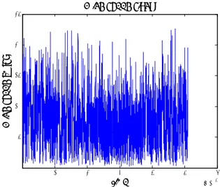
The variability of the wind speed for the two sites is shown in Fig. 1 and Fig. 2. To evaluate the efficiency of the approach that we have proposed, first, the original data is normalized with mean zero and standard deviation equal to one. For each dataset, various experiments were carried out with the use of different architectures and parameters.
0 1 2 3 4 5 6 x 10⁴ 0 5 10 15 20 25 time W ind spe ed (m /s)
Wind speed signal
Fig. 1: Time plot of wind data of Colorado site
0 1 2 3 4 5 6 x 10⁴ 0 5 10 15 20 25 time Wi n d spee d ( m /s)
Wind speed signal
Fig. 2: Time plot of wind data of Connecticut site
In this paper, we use the following error criteria: root mean square error (RMSE), mean absolute error (MAE) and the normalized mean square error (NMSE):
Where NT is the number of test samples; var(y) is the
variance of the output values estimated on all samples,
q
x fˆ is
the value predicted by the model, and yq is the measured
value.
C. Obtained results
4 scenarios for selecting historical time series variables are adopted. In the first one, 50 historical variables are used (full space), in the second, the last four variables are fed to the predictors, in the third and forth one, a PCA and KPCA transformations of the 50 variables are performed before introducing the new PCs to the ELM.
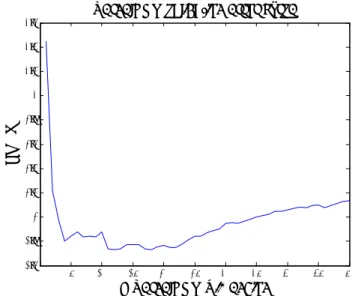
The errors obtained on the validation set is minimized in each case, allows us to have the optimal parameters (hidden nodes and number of principal components) are shown in Fig. 3 to Fig. 6. y't+T=f(yt,yt-1,…..yt-M+1)
RMSE
1
N
T
q
T1 N
f
ˆ
x
q
y
q
2
T NMAE
1
N
T
q1 qy
f
ˆ
x
qNMSE
y
var
1
N
T
q1
f
ˆ
x
q
y
q
2
T N0 5 10 15 20 25 30 35 40 45 50 0.7 0.8 0.9 1 1.1 1.2 1.3 1.4 # Principal Components R M S E
PCA validation error curve
Fig. 3: PCA-ELM validation error curve for wind dataset of Colorado Site
0 5 10 15 20 25 30 35 40 45 50 0.65 0.7 0.75 0.8 0.85 0.9 0.95 1 # KernelPCA Dimension R M S E
KernelPCA validation error curve
Fig. 4: KPCA-ELM validation error curve for Colorado Site
0 5 10 15 20 25 30 35 40 45 50 1.8 2 2.2 2.4 2.6 2.8 3 3.2 3.4 3.6 # Principal Components R M S E
PCA validation error curve
Fig. 5: PCA-ELM validation error curve for Connecticut Site
0 5 10 15 20 25 30 35 40 45 50 1.6 1.8 2 2.2 2.4 2.6 2.8 3 3.2 3.4 3.6 # KernelPCA Dimension R M S E
KernelPCA validation error curve
Fig. 4: KPCA-ELM validation error curve for Connecticut Site
For the sake of comparison, Tables II and IIIshow the results on the two data sets obtained by the different models as well as the corresponding computational time consumed in both learning and test phases using the same computer system.
TABLE II. COLORADO SITE
Dimensionality Reduction technique
Full Space Part of
Space PCA KPCA
Number of variable 50 5 11 12
RMSE 4.3266 15.0364 3.7757 3.0041 NMSE 5.0489 60.9816 3.8450 2.4340 MAE 3.4742 12.0225 3.2799 2.5223 Time(s) 0.9375 0.3906 15.3125 49.9219
TABLE III. CONNECTICUT SITE Dimensionality
Reduction technique
Full Space Part of
Space PCA KPCA
Number of variable 50 5 13 12 RMSE 10.9516 15.3422 6.9959 6.3619 NMSE 6.0453 11.8642 2.4669 2.0400 MAE 9.4312 10.0507 5.9429 5.0572 Time(s) 0.4688 0.3906 15.4531 53.7500 VI. CONCLUSION
A wind speed forecast can lead to an estimate of the expected electrical production of one or more wind turbines (wind farm) in the near future. By production is often meant available power for wind farm considered. Based on the results and discussions presented in this paper, the following conclusions are drawn: First, the KPCA improves the performance of the forecasting process compared to the linear PCA and other variable selection strategies. Second, unlike other neural networks and machine learning techniques, the ELM proved that it has fast convergence and low computational cost. The simulation results on a real datasets show that the proposed approach has a promising potential in
the field of time series forecasting and suitable for online forecasting applications.
REFECENCES
[1] Driss Zejli and Rachid Benchrifa“L’énergie éolienne: de la source d’énergie renouvelable la moins prometteuse à la plus convoitée,” Revue des Energies Renouvelables SMEE’10 pp. 359 – 368 Bou Ismail Tipaza 2010.
[2] Hassen Bouzgou, “A fast and accurate model for forecasting wind speed and solar radiation time series based on extreme learning machines and principal components analysis,” Journal of Renewable and Sustainable Energy, Vol. 6, Issue 1 January 2014.
[3] Mark L. Ahlstrom, and Robert M. Zavadil, “The Role of Wind Forecasting in Grid Operations & Reliability,” IEEE/PES Transmission and Distribution Conference & Exhibition, Asia and Pacific Dalian, China 2005.
[4] Chang, W.-Y. “A Literature Review of Wind Forecasting Methods,” Journal of Power and Energy Engineering, Vol.2, Issue 4, pp.161-168, April 2014.
[5] Saurabh S. Soman, Hamidreza Zareipour, Om Malik and Paras Mandal “A Review of Wind Power and Wind Speed Forecasting Methods with Different Time Horizons,” Conference: North American Power Symposium (NAPS), pp 1-8, September 2010.
[6] Xiaochen Wang, Peng Guoc, Xiaobin Huang “A Review of Wind Power Forecasting Models,” ICSGCE 2011, Chengdu, China, pp. 770-778. September 2011.
[7] Zhang Wei, Wang Weimin, “Wind Speed Forecasting via ensemble Kalman Filter,” The 2nd IEEE International Conference on Advanced Computer Control, Shenyang, China, Vol. 2, p. 73 ,March 2010.
[8] Bouzgou. H, & Benoudjit. N. “Multiple architecture system for wind speed prediction,”. Applied Energy, Vol. 88 Issue 7, pp. 2463-2471, July 2011.
[9] Jong-Min Leea, Chang Kyoo Yoob, Sang Wook Choia, Peter A. Vanrolleghemb, In-Beum Leea; “Nonlinear process monitoring using kernel principal component analysis,” Belgium Chemical Engineering Science, Vol. 59, Issue 1, pp. 223-234, Junuary 2004.
[10] Fauvel, M., Chanussot, J., & Benediktsson, J. A.. “Kernel principal component analysis for feature reduction in hyperspectrale images analysis,” NORSIG 2006. Proceedings of the 7th Nordic pp. 238-24, June 2006.
[11] Guang-Bin Huang, Qin-Yu Zhu, Chee-Kheong Siew, “Extreme learning machine: theory and applications,” Neurocomputing, Vol. 70, Issues 1– 3, pp. 489-501, December 2006.
[12] Peter Zhang “Time series forecasting using a hybrid ARIMA and neural network model,” Neurocomputing, Vol. 50, pp.159-175, January 2003.