Statistical analysis of areal quantities in the brain through permutation tests

(1)

Statistical analysis of

areal quantities in the brain

through permutation tests

dissertation

to obtain the joint degree of Doctor at Maastricht University and Université de Liège,

in Biomedical and Pharmaceutical Sciences.

on the authorities of the Rectores Magnifici, Professor Rianne Letschert and Professor Albert Corhay.

in accordance with the decision of the Board of Deans, to be defended in public on Monday the 10 July 2017 at 16h00.

by

(2)

- Prof. Dr. Gerard J. P. van Breukelen, Maastricht University, The Netherlands - Prof. Dr. Pierre Maquet, Université de Liège, Belgium

- Dr. Edouard Duchesnay, Commissariat à l’énergie atomique et aux énergies altern-atives (cea), France

- Prof. Dr. John Suckling, University of Cambridge, United Kingdom - Dr. Giancarlo Valente, Maastricht University, The Netherlands

The work presented in this thesis was funded by the European Union within the people Programme fp7: Marie Curie Initial Training Networks (fp7-people-itn-2008), Grant Agreement 238593 “Neurophysics”, in which Universiteit Maastricht, Université de Liège, Forschungszentrum Jülich, and GlaxoSmithKline were net-work partners.

(3)

Abstract

In this thesis we demonstrate that direct measurement and comparison across sub-jects of the surface area of the cerebral cortex at a fine scale is possible using mass conservative interpolation methods. We present a framework for analyses of the cortical surface area, as well as for any other measurement distributed across the cortex that is areal by nature, including cortical gray matter volume. The method consists of the construction of a mesh representation of the cortex, registration to a common coordinate system and, crucially, interpolation using a pycnophy-lactic method. Statistical analysis of surface area is done with power-transformed data to address lognormality, and inference is done with permutation methods, which can provide exact control of false positives, making only weak assumptions about the data. We further report on results on approximate permutation meth-ods that are more flexible with respect to the experimental design and nuisance variables, conducting detailed simulations to identify the best method for settings that are typical for imaging scenarios. We present a generic framework for per-mutation inference for complex general linear models (GLMs) when the errors are exchangeable and/or have a symmetric distribution, and show that, even in the presence of nuisance effects, these permutation inferences are powerful. We also demonstrate how the inference on GLM parameters, originally intended for inde-pendent data, can be used in certain special but useful cases in which independence is violated. Finally, we show how permutation methods can be applied to com-bination analyses such as those that include multiple imaging modalities, multiple data acquisitions of the same modality, or simply multiple hypotheses on the same data. For this, we use synchronised permutations, allowing flexibility to integrate imaging data with different spatial resolutions, surface and/or volume-based rep-resentations of the brain, including non-imaging data. For the problem of joint inference, we propose a modification of the Non-Parametric Combination (NPC) methodology, such that instead of a two-phase algorithm and large data storage requirements, the inference can be performed in a single phase, with more reas-onable computational demands. We also evaluate various combining methods and identify those that provide the best control over error rate and power across. We show that one of these, the method of Tippett, provides a link between correction for the multiplicity of tests and their combination.

(4)

(5)

Declaration

I hereby declare that except where specific reference is made to the work of oth-ers, the contents of this dissertation are original and have not been submitted in whole or in part for consideration for any other degree or qualification in these, or any other Universities. This dissertation is the result of my own work and in-cludes nothing which is the outcome of work done in collaboration, except where specifically indicated in the text.

Anderson M. Winkler January 2016

(6)

(7)

Acknowledgements

À minha família.

To the whole network of supervisors and promoters involved in this multi-insti-tutional project, especially Prof. Dr. Thomas E. Nichols and Prof. Dr. Stephen M. Smith, for their effective advisorship.

I am much thankful to the support of Prof. Peter de Weerd, Prof. Andre Luxen, Dr. Philip S. Murphy, and Prof. Paul M. Matthews. I also would like to thank the much helpful assistance of Mr. Ermo Daniëls, Ms. Christl van Veen and Ms. Jeannette Boschma.

I am extremely thankful to the funding provided by the Marie Curie — Initial Train-ing Network (mc-itn) “Methods in NeuroimagTrain-ing”, through its four core partners, Universiteit Maastricht, Université de Liège, Forschungszentrum Jülich and Glaxo-SmithKline.

Some chapters benefited from strong, prolific, and enriching collaboration. The work on areal interpolation (Chapter 2) would have been impossible without the help of, first and foremost, David C. Glahn. I am also much thankful to Mert R. Sabuncu, B. T. Thomas Yeo, Bruce Fischl, Douglas N. Greve, Peter Kochunov, and John Blangero. The work on permutation for the general linear model (Chapter 3) greatly benefited from the participation of Gerard R. Ridgway and Matthew A. Webster. The work on combined inference (Chapter 4) was much improved thanks to the participation of Matthew A. Webster, Jonathan C. Brooks and Irene Tracey.

(8)

(9)

Propositions

In complement of the dissertation:

Statistical analysis of areal quantities in the brain through permutation tests

by Anderson M. Winkler

Propositions 1–4 are related to the subject matter of the dissertation; Propositions 3–7 are related to the subject field of the doctoral candidate; Proposition 8 is not related to either.

1. Analysis of brain cortical surface area has received insufficient attention com-pared to thickness and volume, even though it provides a different kind of in-formation about the cortex, particularly when compared to thickness.

2. Pycnophylactic interpolation is the most appropriate method to resample areal quantities to allow comparisons between individuals.

3. The G-statistic provides a simple generalisation over various well known stat-istics. Written in matrix form, it can be computed quickly for imaging data, and assessed through permutations, sign flippings, or permutations with sign flippings, either freely or with restrictions imposed by exchangeability blocks, depending on knowledge or assumptions about the data and residuals.

4. Non-parametric combination can be modified so as to run in a single phase, rendering its use feasible for imaging data, and offering in general higher power compared to classical multivariate tests.

5. Voxel-based morphometry (vbm) had its time, but should no longer be used for serious research of cortical anatomy, particularly given that other methods are readily available.

6. Cortical surface area at finer resolution can provide adequate traits that are closer to gene action and may be more successful for the identification of genes that influence brain structure and function.

7. Cortical surface area is heritable and has potential to be an endophenotype for psychiatric disorders.

8. Knowledge of genetic influences on brain structure and function should be used to fight disease and improve quality of life. Its influences on policy making, however, must be seen with caution, and receive due, wide consideration.

(10)

(11)

List of Figures

1.1 Some possible analyses of cortical morphometric measurements

using permutation tests. . . 20

2.1 Surface- and volume-based representations of the cortex. . . 26

2.2 Example demonstrating differences between area and point meas-urements. . . 28

2.3 Overview of areal analyses. . . 30

2.4 Overlapping areas used to weight areal quantities during interpol-ation. . . 34

2.5 Geodesic spheres. . . 38

2.6 Differences between presentation of facewise and vertexwise area. 42 2.7 Effect of registration method on areal analyses. . . 45

2.8 The distribution of surface area is lognormal. . . 47

2.9 Results of the Shapiro–Wilk normality test. . . 48

2.10 Maps of the skewness of the areal data. . . 49

2.11 Histograms of the skewness of the areal data. . . 50

2.12 Maps of the kurtosis of the areal data. . . 51

2.13 Histograms of the kurtosis of the areal data. . . 52

2.14 Spatial distribution of the parameter λ. . . . 53

2.15 Example of a retessellated surface. . . 55

2.16 Comparison with expansion/contraction methods (i). . . 57

2.17 Comparison with expansion/contraction methods (ii). . . 58

2.18 Comparison with expansion/contraction methods (iii). . . 59

3.1 Examples of permutation and sign flipping matrix. . . 75 13

(16)

4.2 Overview of the original and modified npc . . . 140

4.3 Rejection regions of two partial tests with four different combining functions. . . 142

4.4 Examples of inconsistent combining functions. . . 144

4.5 Examples of inadmissible combining functions. . . 146

4.6 Overview of the main simulation parameters. . . 156

4.7 Histograms of p-values for the simulations. . . 159

4.8 Bland–Altman plots comparing original and modified npc. . . 160

4.9 Performance of the modified npc using different combining func-tions, compared to Hotelling’s T2_{. . . 162}

4.10 Results of the example pain study. . . 164

(17)

List of Tables

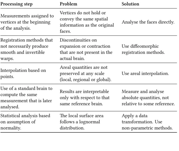
2.1 Problems solved by the proposed method. . . 55

2.2 Stability of areal measurements. . . 60

3.1 Summary of assumptions of permutation methods. . . 82

3.2 Methods available to construct the null distribution in the presence of nuisance variables. . . 83

3.3 Some tests of which the statistic G is a generalisation. . . . 86

3.4 Maximum number of unique permutations. . . 88

3.5 Coding for Example 1 . . . 94

3.11 Summary of simulation scenarios. . . 101

3.12 False positive rate and power for the statistics F and G. . . 106

3.13 Summary of the amount of error type i and power for the different permutation strategies. . . 107

3.14 Amount of error type i for representative simulation scenarios. . 107

4.1 Summary of various combining functions . . . 119

4.2 Joint hypotheses of uit and iut. . . 126

(18)

(19)

Chapter 1 Introduction

It has been suggested that the processes that drive horizontal (tangential) and vertical (radial) development of the cerebral cortex are separate from each other (Rakic, 1988). Variations on these would result, respectively, in variations on the extent of cortical surface area and on the thickness of the cortical mantle. Through the use of genetically informative samples, it has been demonstrated these two processes are indeed uncorrelated genetically (Panizzon et al., 2009; Winkler et al., 2010) and are each influenced by regionally distinct genetic factors (Schmitt et al., 2008; Rimol et al., 2010b). Moreover, it is variation on surface area that explains most of the variation observed in the amount of gray matter assessed with meth-ods that only measure volume, such as voxel-based morphometry (Winkler et al., 2010; Rimol et al., 2012).

These findings give prominence to the use of surface area alongside cortical thickness in studies of brain morphology and, and its interaction with brain func-tion. However, cortical surface area been measured only over gross regions or approached indirectly via comparisons with a standard brain. Of studies using the latter, few that have used area measurements on every point of the cortex (vertex-wise) and have offered detailed insight on the exact procedures used for this assess-ment. Some studies described their methods in terms of “expansion/contraction”, often using different definitions of what expansion or contraction would be. By 2011, various impromptu approaches had been considered, for example:

– Lyttelton et al. (2009): The authors describe that the asymmetry measure-ment is the logarithm of the ratio of the area per vertex of left and right

(20)

– Sun et al. (2009a): The authors state that “The distance between a center po-sition of the brain (…) and each brain surface point was calculated (…). The difference of the above radial distances between the follow-up and baseline brain surfaces (…) was defined as brain surface contraction”. Under this definition, not only contraction refers to an initial point in time, but it also refers not to a bidimensional feature, and instead to a linear distance between each point in the surface and a given central point in the brain.

– Sun et al. (2009b): The authors state that “The distance between two brain surfaces [i.e. inner skull and pial] was then measured at subvoxel resolution (…), the value in millimeters was assigned to the voxel as the intensity value and an image of the brain surface contraction was obtained”. Under this definition, for a longitudinal study, the contraction is the difference between initial and final distances between inner skull and pial surfaces, assigned to a volumetric (voxel-based) space.

– Hill et al. (2010): The article discusses growth of the cortex from birth to adulthood and compares it with the cortex of the monkey. Here expansion can be interpreted as in relation to an initial, developmental and/or evolu-tionary stage, not to a given template or to the other hemisphere.

– Rimol et al. (2010a): Expansion and contraction are measured in relation to a template, as in Joyner et al. (2009).

– Palaniyappan et al. (2011): The authors state that “In line with Joyner et al. (2009), we use the term contraction to suggest group differences in the sur-face area in patients compared to controls, rather than a reduction from pre-viously larger area.” This in fact seems a new interpretation over the method

(21)

19

used by Joyner et al. (2009), as the authors here would then be using expan-sion/contraction to compare to the control group. Yet, reading through the article, it appears clear that expansion/contraction still refers to the chosen template.

– Chen et al. (2011, 2012): The authors use a method similar to Joyner et al. (2009) and Rimol et al. (2010a), and so, expansion/contraction refer to the template.

All these different operating definitions of what expansion/contraction would be create already difficulties in the interpretation of their meaning. However, even if only one of these existed, it would still be difficult to interpret, due to the depend-ence of all these methods on a referdepend-ence brain or on the contra-lateral hemisphere, from which expansion or contraction is tentatively assessed.

In the present work, we propose a method that uses absolute quantities, as op-posed to being relative to a reference brain. While initially addressing these con-cerns, we found yet others that required further investigation. The first is that we found that surface area is lognormally distributed, such that direct use of statistical methods based on the assumption of normality are likely to yield incorrect results. The second concerns use of data assigned to each face of a mesh representation of the brain, as opposed to each vertex, which cannot be analysed in software designed to handle vertexwise data, nor stored in vertexwise file formats, thus demanding the development of new tools for analysis and a file format. The third is that in neuroimaging thousands of tests are performed in an image representation of the brain. None of the parametric methods can be considered for control of the fami-lywise error rate, given the lognormality and the spatial dependencies among the data assigned to each face of the mesh representation without appealing to many unrealistic assumptions, thus demanding the use of more flexible approaches.

Treating these problems eventually that led into a complete framework for the measurement and statistical analysis of areal quantities. It uses permutation tests in the general linear model, and yet allowing area and thickness to be studied jointly without appealing to cortical volume. Nonetheless, the method can also be used to study volume, either using the current approach of multiplying cortical area by cortical thickness, or else, using an improved method that we propose, in

(22)

(via permutations) Thickness

Figure 1.1: Some possible analyses of cortical morphometric measurements using per-mutation tests. Inter-subject comparisons of cortical area and other areal quantities, such as volume, that depends on both area and thickness, use the methods proposed in Chapter 2. Univariate statistical analysis of each of these separately use the strategy dis-cussed in Chapter 3. Joint (combined) analysis of area and thickness, that bypass volumes altogether, would use the methods proposed in Chapter 4, in particular the non-parametric combination (npc), but also classical multivariate tests.

which no pieces of the cortex are left over- or under-represented.

Although this work can be organised into three core topics that are relatively independent from each other, and that have each been published as separate pa-pers (Winkler et al., 2012, 2014, 2016), the flow of information in a complete study of cortical morphology visits all three, as shown in Figure 1.1. The next sections outline these three main chapters. Each chapter offers a detailed introduction de-scribing the problem that each aim to solve, along with review of the relevant literature, evaluation and implementation, including algorithms as needed, and a detailed discussion.

1.1 Methods for areal quantities

The general strategy for analyses of cortical measurements consists of the gener-ation of a surface-representgener-ation of the brain and its subsequent transformgener-ation into a sphere. Vertices of this sphere are then shifted along its surface to allow alignment that matches some feature of interest, such as sulcal depth, myelin

(23)

con-1.2. Methods for permutation inference 21

tent, or functional markers. As the alignment is performed, quantities assigned to vertices or faces, such as thickness or area, are carried along these vertices and faces. Once registration is done, these quantities are interpolated to a common grid (mesh), where comparisons between subjects can be performed.

While methods to study thickness across subjects are available (Fischl and Dale, 2000), and use interpolation to a common reference grid using methods such as nearest neighbour or barycentric, such interpolation strategies cannot be used for either cortical area itself, nor to other areal quantities, such as cortical volume, as these are not mass-conservative (pycnophylactic). Chapter 2 clarifies the dis-tinction between the nature of these measurements, and proposes the use of areal interpolation. This strategy permits quantities to be studied in absolute terms, as opposed to relative to some reference brain. The chapter proposes that areal quant-ities are analysed directly in the faces of the mesh from which they were computed, instead of resampled to vertices, which halves the resolution.

We demonstrate that areal data do not follow a normal distribution, being bet-ter characbet-terised by a mixture of normal and lognormal distributions, in propor-tions that vary across the brain and possibly according to the scale of measurement. A power transformation can be considered to address lognormality, although a better alternative is to use permutation methods, that not only do not rely on dis-tributional assumptions, but also allow correction for multiple testing and the use of non-standard statistics.

1.2 Methods for permutation inference

Permutation methods can provide exact control of false positives, making only weak assumptions about the data, and have been available in brain imaging for many particular cases (Holmes et al., 1996; Nichols and Holmes, 2002), although no implementation for surface-based methods, even less so for facewise data as we have developed, existed in the literature until this work. With the recent avail-ability of fast and inexpensive computing, the main limitation of permutation tests would be a certain lack of flexibility with respect to arbitrary experimental designs, in particular with respect to nuisance variables in the model, as well as repeated measurements.

(24)

provide control of false positives in a wide range of common and relevant imaging research scenarios.

We also demonstrate how the inference on glm parameters, originally inten-ded for independent data, can be used in certain special but useful cases in which independence is violated, by means of using exchangeability blocks, that is, sets of observations with shared non-independence, and that can sometimes be treated as a single unit for permutation, i.e., shuffled as a whole, or sometimes serve as delimiters such that permutations happen only within block. The definition of ex-changeability blocks allow for groups of observations with same variances, either known or assumed, thus requiring a statistic that preserves certain desirable prop-erties for control of multiple testing even under such scenarios. We provide such a statistic, dubbed G-statistic, which is a generalisation of the F -statistic, as well as others.

1.3 Methods for joint permutation inference

While gray matter volume can be studied directly using the methods discussed in Chapter 2, it may be the case that true effects affecting thickness and area in oppos-ite directions may cancel each other. Yet, analysing them separately using univari-ate methods as in Chapter 3 may not aggregunivari-ate power from having effects acting simultaneously on both. Likewise, participants of an imaging study are often sub-jected to the acquisition of more than one imaging modality. These modalities are often analysed separately. However, a joint analysis has potential to answer more complex questions and to increment power. Moreover, even a single modality can sometimes be partitioned into subcomponents that disentangle different aspects of brain structure or function. Examples include independent component analysis, as

(25)

1.3. Methods for joint permutation inference 23

well as scalar measurements from diffusion-tensor imaging.

In Chapter 4 we show how permutation methods can be applied to combin-ation analyses such as those that include multiple imaging modalities, multiple data acquisitions of the same modality, or simply multiple hypotheses on the same data. Using the well-known definition of union-intersection tests and closed test-ing procedures, we use synchronised permutations to correct for such multipli-city of tests, allowing flexibility to integrate imaging data with different spatial resolutions, surface and/or volume-based representations of the brain, including non-imaging data.

In particular for the problem of joint inference, we propose and evaluate a modification of the recently introduced Non-Parametric Combination (npc) meth-odology (Pesarin and Salmaso, 2010a), such that instead of a two-phase algorithm and large data storage requirements, the inference can be performed in a single phase, with reasonable computational demands. We also evaluate, in the context of permutation tests, various combining methods that have been proposed in the past decades, and identify those that provide the best control over error rate and power across a range of situations. We show that one of these, the method of Tippett (1931), provides a link between correction for the multiplicity of tests and their combination.

Finally, we discuss how the correction can solve certain problems of multiple comparisons in common designs, and how the combination is distinguished from conjunctions, even though both can be assessed using permutation tests. We also provide a common algorithm that accommodates combination and correction.

(26)

(27)

Chapter 2 Areal quantities in the cortex

2.1 Introduction

The surface area of the cerebral cortex greatly differs across species, whereas the cortical thickness has remained relatively constant during evolution (Mountcastle, 1998; Fish et al., 2008). At a microanatomic scale, regional morphology is closely related to functional specialization (Roland and Zilles, 1998; Zilles and Amunts, 2010), contrasting with the columnar organization of the cortex, in which cells from different layers respond to the same stimulus (Jones, 2000; Buxhoeveden and Casanova, 2002). In addition, Rakic (1988) proposed an ontogenetic model that ex-plains the processes that lead to cortical arealization and differentiation of cortical layers according to related, yet independent mechanisms. Supporting evidence for this model has been found in studies with both rodent and primates, including hu-mans (Chenn and Walsh, 2002; Rakic et al., 2009), as well as in pathological states (Rimol et al., 2010a; Bilgüvar et al., 2010).

At least some of the variability of the distinct genetic and developmental pro-cesses that seem to determine regional cortical area and thickness can be captured using polygon mesh (surface-based) representations of the cortex derived from T1

-weighted magnetic resonance imaging (mri) (Panizzon et al., 2009; Winkler et al., 2010; Sanabria-Diaz et al., 2010). In contrast, volumetric (voxel-based) representa-tions, also derived from mri, were shown to be unable to readily disentangle these processes (Winkler et al., 2010). Figure 2.1 shows schematically the difference between these two representations.

(28)

Surface area

Figure 2.1: Geometrical relationship between cortical thickness, surface area and grey matter volume. In the surface-based representation, the grey matter volume is a quad-ratic function of distances in the surfaces and a linear function of the thickness. In the volume-based representation, only the volumes can be measured directly and require par-tial volume-effects to be considered (Winkler et al., 2010).

Mesh representations of the brain allow measurements of the cortical thick-ness at every point in the cortex, as well as estimation of the average thickthick-ness for pre-specified regions. However, to date, analyses of cortical surface area have been generally limited to two types of studies: (1) vertexwise comparisons with a standard brain, using some kind of expansion or contraction measurement, either of the surface itself (Joyner et al., 2009; Lyttelton et al., 2009; Hill et al., 2010; Rimol et al., 2010a; Palaniyappan et al., 2011), of linear distances between points in the brain (Sun et al., 2009a,b), or of geometric distortion (Wisco et al., 2007), or (2) ana-lyses of the area of regions of interest (roi) defined from postulated hypotheses or from macroscopic morphological landmarks (Dickerson et al., 2009; Nopoulos et al., 2010; Kähler et al., 2011; Durazzo et al., 2011; Schwarzkopf et al., 2011; Eyler et al., 2011; Chen et al., 2011, 2012). Analyses of expansion, however, do not deal with area directly, depending instead on non-linear functions associated with the warp to match the standard brain, such as the Jacobian of the transformation. Moreover, by not quantifying the amount of area, these analyses are only interpretable with respect to the brain used for the comparisons. Roi-based analyses, on the other hand, entail the assumption that each region is homogeneous with regard to the feature under study, and have maximum sensitivity only when the effect of interest is present throughout the roi.

(29)

2.2. Method 27

These difficulties can be obviated by analysing each point on the cortical surface of the mesh representation, a method already well established for cortical thick-ness (Fischl and Dale, 2000). Pointwise measurements, such as thickthick-ness, are gener-ally taken at and assigned to each vertex of the mesh representation of the cortex. This kind of measurement can be transferred to a common grid and subjected to statistical analysis. Standard interpolation techniques, such as nearest neighbor, barycentric (Yiu, 2000), spline-based (De Boor, 1962) or distance-weighted (Shep-ard, 1968) can be used for this purpose. The resampled data can be further spatially smoothed to alleviate residual interpolation errors. However, this approach is not suitable for areal measurements, since area is not inherently a point feature. To illustrate this aspect, an example is given in Figure 2.2. Methods that can be used for interpolation of point features do not necessarily compensate for inclusion or removal of datapoints,¹ unduly increasing or reducing the global or regional sum of the quantities under study, precluding them for use with measurements that are, by nature, areal. The main contribution of this chapter is to address the technical difficulties in analysing the local brain surface area, as well as any other cortical quantity that is areal by nature. We propose a framework to analyse areal quant-ities and argue that a mass preserving interpolation method is a necessary step. We also study different processing strategies and characterize the distribution of facewise cortical surface area.

2.2 Method

An overview of the method is presented in Figure 2.3. Comparisons of cortical area between subjects require a surface model for the cortex to be constructed. A number of approaches are available (Mangin et al., 1995; Dale et al., 1999; van Essen et al., 2001; Kim et al., 2005) and, in principle, any could be used. Here we adopt the method of Dale et al. (1999) and Fischl et al. (1999a), as implemented in the FreeSurfer software package (fs).² In this method, the T1-weighted images

¹ A notable exception is the natural neighbor method (Sibson, 1981). However, the original method needs modification for use with areal analyses.

(30)

to be collected include the number of trees of a certain slow growing species, and the depth of the soil until a specific rocky formation is found. They prepare a trip to the field for data collection.

Figure 2.2: An example demonstrating differences in the nature of measurements. In this analogy, the depth of the soil is similar to brain cortical thickness, whereas the number of trees is similar to areal quantities distributed across the cortex. These areal quantities can be the surface area itself (in this case, the area of the terrain), but can also be any other measurement that is areal by nature (such as the number of trees).

(31)

2.2. Method 29

are initially corrected for magnetic field inhomogeneities and skull-stripped (Sé-gonne et al., 2004). The voxels belonging to the white matter (wm) are identified based on their locations, on their intensities, and on the intensities of the neigh-boring voxels. A mass of connected wm voxels is produced for each hemisphere, using a six-neighbors connectivity scheme, and a mesh of triangular faces is tightly built around this mass, using two triangles per exposed voxel face. The mesh is smoothed taking into account the local intensity in the original images (Dale and Sereno, 1993), at a subvoxel resolution. Topological defects are corrected (Fischl et al., 2001; Ségonne et al., 2007) ensuring that the surface has the same topological properties of a sphere. A second iteration of smoothing is applied, resulting in a realistic representation of the interface between gray and white matter (the white surface). The external cortical surface (the pial surface), which corresponds to the pia mater, is produced by nudging outwards the white surface towards a point where the tissue contrast is maximal, maintaining constraints on its smoothness and on the possibility of self-intersection (Fischl and Dale, 2000). The white surface is inflated in an area-preserving transformation and subsequently homeomorph-ically transformed to a sphere (Fischl et al., 1999b). After the spherical transform-ation, there is a one-to-one mapping between faces and vertices of the surfaces in the native geometry (white and pial) and the sphere. These surfaces are comprised exclusively of triangular faces.

2.2.1 Area per face and other areal quantities

The surface area for analysis is computed at the interface between gray and white matter, i.e. at the white surface. Another possible choice is to use the middle surface, i.e. a surface that runs at the mid-distance between white and pial. Although this surface is not guaranteed to match any specific cortical layer, it does not over or under-represent gyri or sulci (van Essen, 2005), which might be an useful property. The white surface, on the other hand, matches directly a morphological feature and also tends to be less sensitive to cortical thinning or thickening than the middle or pial surfaces. Whenever methods to produce surfaces that represent biologically meaningful cortical layers are available, these should be preferred.

(32)

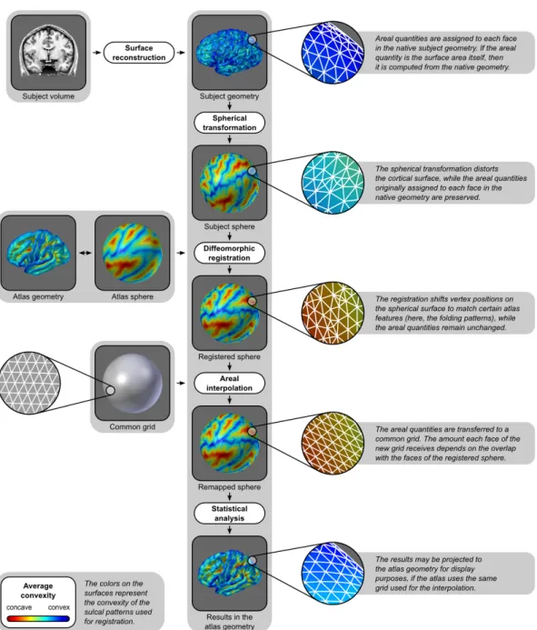
Figure 2.3: Diagram of the steps to analyse the cortical surface area. For clarity, the colors represent the convexity of the surface, as measured in the native geometry.

(33)

2.2. Method 31

at a given vertex is summed and divided by three, producing a measure of the area per vertex, for facewise analysis it is the area per face that is measured and analysed. Since for each subject, each face in the native geometry has its corres-ponding face on the sphere, the value that represents area per face, as measured from the native geometry, can be mapped directly to the sphere, despite any areal distortion introduced by the spherical transformation.

Furthermore, since there is a direct mapping that is independent of the ac-tual area in the native geometry, any other quantity that is biologically areal can also be mapped to the spherical surface. Perhaps the most prominent example is cortical volume (Section 2.2.3), although other cases of such quantities, that may potentially be better characterized as areal processes, are the extent of the neural activation as observed with functional mri, the amount of amyloid deposited in Alzheimer’s disease (Klunk et al., 2004; Clark et al., 2011), or simply the the number of cells counted from optic microscopy images reconstructed to a tri-dimensional space (Schormann and Zilles, 1998). Since areal interpolation (described below) conserves locally, regionally and globally the quantities under study, it allows ac-curate comparisons and analyses across subjects for measurements that are areal by nature, or that require mass conservation on the surface of the mesh represent-ation.

2.2.2 Computation of surface area

The facewise areas in the mesh representation of the brain can be computed trivi-ally: for a triangular face ABC with vertices a = [xA yA zA]′, b = [xB yB zB]′,

and c = [xC yC zC]′, the area is|u×v|/2, where u = a−c, v = b−c, × represents

the cross product, and| • | represents the vector norm.

2.2.3 Volume as an areal quantity

Gray matter volume can be assessed using the partial volume effects of the gray matter in a per-voxel fashion using volume-based representations of the brain, such as in voxel-based morphometry (vbm Ashburner and Friston, 2000), or as the amount of tissue present between the gray and white surfaces in surface-based representations. Using the surface-based representation, software such as

(34)

Free-across subjects (Drury et al., 1996). The registration is performed by shifting vertex positions along the surface of the sphere until there is a good alignment between subject and template (target) spheres with respect to certain specific features, usu-ally, but not necessarily, the cortical folding patterns. As the vertices move, the areal quantities assigned to the corresponding faces are also moved along the sur-face. The target for registration should be the less biased as possible in relation to the population under study (Thompson and Toga, 2002).

A registration method that produces a smooth, i.e. spatially differentiable, warp function enables the smooth transfer of areal quantities. A possible way to ac-complish this is by using registration methods that are diffeomorphic. A diffeo-morphism is an invertible transformation that has the elegant property that it and its inverse are both continuously differentiable (Christensen et al., 1996; Miller et al., 1997), minimising the risk of vagaries that would be introduced by the non-differentiability of the warp function.

Diffeomorphic methods are available for spherical meshes (Glaunès et al., 2004; Yeo et al., 2010a; Robinson et al., 2014), and here we adopt the Spherical Demons (sd) algorithm³ (Yeo et al., 2010a). Sd extends the Diffeomorphic Demons algorithm (Vercauteren et al., 2009) to spherical surfaces. The Diffeomorphic Demons al-gorithm is a diffeomorphic variant of the efficient, non-parametric Demons regis-tration algorithm (Thirion, 1998). Sd exploits spherical vector spline interpolation theory and efficiently approximates the regularization of the Demons objective function via spherical iterative smooting.

Methods that are not diffeomorphic by construction (Fischl et al., 1999b; Auzias

(35)

2.2. Method 33

et al., 2013), but in practice produce invertible and smooth warps could, in prin-ciple, be used for registration for areal analyses. In the Evaluation section we study the performance of different registration strategies as well as the impact of the choice of the template.

2.2.5 Areal interpolation

After the registration, the correspondence between each face on the registered sphere and each face from the native geometry is maintained, and the surface area or other areal quantity under study can be transferred to a common grid, where statistical comparisons between subjects can be performed. The common grid is a mesh which vertices lie on the surface of a sphere. A geodesic sphere, which can be constructed by iterative subdivision of the faces of a regular icosahedron, has many advantages for this purpose, namely, ease of computation, edges of roughly similar sizes and, if the resolution is fine enough, edge lengths that are much smaller than the diameter of the sphere (see Section 2.2.7 for details). These two spheres, i.e. the registered, irregular spherical mesh (source), and the common grid (target), typically have different resolutions. The interpolation method must, nevertheless, conserve the areal quantities, globally, regionally and locally. In other words, the method has to be pycnophylactic⁴ (Tobler, 1979). This is accomplished by assigning, to each face in the target sphere, the areal quantity of all overlapping faces from the source sphere, weighted by the fraction of overlap between them (Figure 2.4).

More specifically, let QS

i represent the areal quantity on the i-th face of the

registered, source sphere S, i = 1, 2, . . . , I. This areal quantity can be directly mapped back to the native geometry, and can be the area per face as measured in the native geometry, or any other quantity of interest that is areal by nature. Let the actual area of the same face on the source sphere be indicated by AS

i. The

quantities QS

i have to be transfered to a target sphere T , the common grid, which

face areas are given by AT

j for the j-th face, j = 1, 2, . . . , J, J ̸= I. Each target

face j overlaps with K faces of the source sphere, being these overlapping faces

⁴ From Greek pyknos = mass, density, and phylaxis = guard, protect, preserve, meaning that the method has to be mass conservative.

(36)

utes an amount of areal quantity. This amount is determined by the proportion between each overlapping area (represented in different colors) and the area of the respective source face. (c) The interpolation is performed at multiple faces of the target surface, so that the amount of areal quantity assigned to a given source face is conservatively redistributed across one or more target faces.

indicated by indices k = 1, 2, . . . , K, and the area of each overlap indicated by AO k.

The interpolated areal quantity to be assigned to the j-th target face is then given by: QT_j = K ∑ k=1 AO_k AS k QS_k (2.1)

Similar interpolation schemes have been devised to solve problems in geo-graphic information systems (gis) (Markoff and Shapiro, 1973; Goodchild and Lam, 1980; Flowerdew et al., 1991; Gregory et al., 2010). Surface models of the brain im-pose at least one additional challenge, which we address in the implementation (see Section 2.2.6). Differently than in other fields, where interpolation is performed over geographic territories that are small compared to Earth and, therefore, can be projected to a plane with acceptable areal distortion, here we have to interpolate across the whole sphere. Although other conservative interpolation methods exist for this purpose (Jones, 1999; Lauritzen and Nair, 2008; Ullrich et al., 2009), these methods either use regular latitude-longitude grids, cubed-spheres, or require a special treatment of points located above a certain latitude threshold to avoid sin-gularities at the poles. These disadvantages may render these methods suboptimal for direct use in brain imaging.

(37)

2.2. Method 35

2.2.6 Implementation

The areal interpolation for spheres is implemented in two parts. In the first, we compute inside of which source faces the target vertices are located, creating a lookup table to be used in the second part. This is the point-in-polygon prob-lem found in vector graphics applications (Vince, 2005). Here we calculate the area of each source face, AS

i, and the subsequent steps proceed iteratively for each

face in the source. The barycentric coordinates of each candidate vertex in rela-tion to the current face i is computed; if their sum equals to unity, the point is labelled as inside. However, to test if all vertices are inside every face would need-lessly waste computational time. Moreover, since all points are on the surface of a sphere, the vertices in the target are never expected to be coplanar to the source triangular faces, so the test would always fail. The first problem is treated by test-ing only the vertices located within a boundtest-ing box defined, still in the 3d space, from the source face extreme coordinates. The second could naïvely be treated by converting the 3d Cartesian coordinates to 2d spherical coordinates, which allow a fast flattening of the sphere to the popular plate carrée cylindrical projection. However, latitude is ill-defined at the poles in cylindrical projections. Moreover, cylindrical projections introduce a specific type of deformation that is undesired here: straight lines on the surface (geodesic lines) are distorted. The solution we adopt is to rotate the Cartesian coordinate system so that the barycenter of the current source face lies at the point [r 0 0]′_{, where r is the radius of the source}

and target spheres. The barycenter is used for ease of calculation and for being al-ways inside the triangle. After rotation, the current face and the nearby candidate target vertices are projected to a plane using the azimuthal gnomonic projection (Snyder, 1987), centered at the barycenter of the face. The point-in-polygon test can then be applied successfully. The key advantage of the gnomonic projection is that all geodesics project as straight lines, rather than loxodromic or other com-plex paths as with other projections, which would cause many target vertices to be incorrectly labelled. This projection can be obtained trivially after the rotation of the 3d Cartesian coordinate system as ϕ = y/x and θ = z/x, where [x y z]′

are the 3d coordinates of the point being projected. A potential disadvantage of the gnomonic projection is the remarkable areal distortion for regions distant from

(38)

tion depends on optimally finding crossings between multiple line segments (Bent-ley and Ottmann, 1979; Chazelle and Edelsbrunner, 1992; Balaban, 1995). Most of the efficient available algorithms assume that the polygons are all coplanar; those that work in the surface of a sphere use coordinates expressed in latitude and lon-gitude and require special treatment of the polar regions. The solution we adopt obviates these problems by first computing the area of each target face, AT

j; the

subsequent steps are performed iteratively for each face in the target sphere, using the azimuthal gnomonic projection, similarly as in the first part, but now centered at the barycenter of the current target face at every iteration. The areal quantities assigned to the faces in the target sphere are initialized as zero before the loop begins. If all three vertices of the current target face j lie inside the same source face k, as known from the lookup table produced in the first part, then to the cur-rent face the areal quantity given by QT

j = QSkA

T

j/ASk is assigned. Otherwise, the

source faces that surround the target are examined to find overlaps. This is done by considering the edges of the current target face as vectors organised in counter-clockwise orientation, and testing if the vertices of the candidate faces lie on the left, right or if they coincide with the edge. If all the three vertices of any candid-ate face are on the right of any edge, there is no overlap and the candidcandid-ate face is removed from further consideration. If all the three vertices are on the left of all three edges, then the candidate source face is entirely inside the target, which has then its areal quantity incremented as QT

j ← QTj + QSk. The remaining faces are

those that contain some vertices on the left and some on the right of the edges of the current, target face. The intersections between these source and target edges are computed and false intersections between edge extensions are ignored. A list containing the vertices for each candidate source face that are inside the target face (known for being on the left of the three target edges), the target vertices that are

(39)

2.2. Method 37

inside each of the source faces (known from the lookup table) and the coordinates of the intersections between face edges, is used to compute the convex hull, using the Quickhull algorithm (Barber et al., 1996). The convex hull delimits the over-lapping region between the current target face j and the candidate source face k, which area, AO

k, is used to increment the areal quantity assigned to the target face

as QT

j ← QTj + QSkAOk/ASk.

The algorithm runs in O(n) for n faces, as opposed to O(n2₎ _{that would be}

obtained by naïve search. Nevertheless, the current implementation, that runs in Octave (Eaton et al., 2015) or matlab (The MathWorks Inc., 2015), a dynamically typed, interpreted language, requires about 24 hours to run in a computer with 2.66 GHz Intel Xeon processors.

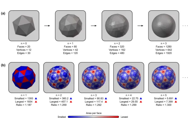
2.2.7 Geodesic spheres and areal inequalities

The only required feature for the common grid used for the areal interpolation is that all its vertices must lie on the surface of a sphere. The algorithm we present in Section 2.2.6 requires further that all faces of the sphere are triangular and that all edges of all faces are much smaller than the radius, so that areal distortion is minimised when projecting to a plane.

A common grid that meet these demands is a sufficiently fine geodesic sphere. There are different ways to construct such a sphere (Kenner, 1976). One method is to subdivide each face of a regular polyhedron with triangular faces, such as the icosahedron, into four new triangles. The new vertices are projected to the surface of the (virtual) circumscribed sphere along its radius and the process is repeated recursively a number of times (Lauchner et al., 1969). For the n-th iteration, the number of faces is given by F = 4n_F

0, the number of vertices by V = 4n(V0−2)+

2, and the number of edges by E = 4n_E

0, where F0, V0and E0are, respectively, the

number of faces, vertices and edges of the polyhedron with triangular faces used for the initial subdivision. For the icosahedron, F0 = 20, V0 = 12 and E0 = 30

(Figure 2.5a). For the analyses in this manuscript, we used n = 7, producing geodesic spheres with 327680 faces and 163842 vertices.

These faces, however, do not have identical edge lengths and areas (Kenner, 1976), even though the initial icosahedron was perfectly regular. This is

(40)

import-Figure 2.5: (a) The common grid can be a geodesic sphere produced from recursive subdi-vision of a regular icosahedron. At each iteration, the number of faces is quadruplied. (b) After the first iteration, however, the faces no longer have regular sizes, with the largest face being approximately 1.3 times larger than the smallest as n increases.

ant for areal interpolation, as larger faces on the target grid do overlap with more faces from the source surfaces, absorbing larger amounts of areal quantities, pos-sibly causing confusion if one attempts to color-encode the interpolated image according to the actual areal quantities, in which case, geometric patterns such as in Figure 2.5b will become evident. Moreover, smoothing can cause quantities that are arbitrarily large or small due to face sizes to be blurred into the neighbors. Both potential problems can be addressed by multiplying the areal quantity at each face j, after interpolation, by a constant given by 4πr2_/(AT

jF ), where ATj is the area of

the same face of the geodesic sphere, F is the number of faces, and r is the radius of the sphere.

2.2.8 Smoothing

Smoothing can be applied to alleviate residual discontinuities in the interpolated data due to unfavorable geometric configurations between faces of source and tar-get spheres. For the purpose of smoothing, facewise data can be represented either by their barycenters, or converted to vertexwise (see Section 2.2.11 for a discussion

(41)

2.2. Method 39

on how to convert), and should take into account differences on face sizes, as lar-ger faces will tend to absorb more areal quantities (see Section 2.2.7). Smoothing can be applied using the moving weights method (Lombardi, 2002), defined as

˜ QT_n = ∑ jQ T jG(g(xn,xj)) ∑ jG(g(xn,xj)) (2.2) where ˜QT

n is the smoothed areal quantity at the n-th face, QTj is the areal quantity

assigned to each of the J faces of the same surface before smoothing, g(xn,xj)is

the scalar-valued distance along the surface between the barycenter xnof the

cur-rent face and the barycenter xj of another face, and G(g) is the Gaussian kernel.⁵

2.2.9 Conversion from facewise to vertexwise

Whenever it is necessary to perform analyses that include measurements taken at each vertex (such as some areal quantity versus cortical thickness) or when only software that can display vertexwise data is available (Section 2.2.11, it may be ne-cessary to convert the areal quantities from facewise to vertexwise. The conversion can be done by redistributing the quantities at each face to their three constitu-ent vertices. The areal values assigned to the faces that meet at a given vertex are summed, and divided by three, and reassigned to this vertex. Importantly, this pro-cedure has to be done after the areal interpolation, since interpolation methods for vertexwise data are not appropriate for areal quantities, and before the statistical analysis, since the average of the results of the statistics of a test is not necessar-ily the same as the statistic for the average of the original data. It should also be observed that conversion from facewise to vertexwise data implies a loss of res-olution to approximately half of the original and, therefore, should be performed only if resolution is not a concern and there is no other way to analyse, visualize, or present facewise data or results. The conversion does not change the underlying distribution, provided that the resolution of the initial mesh is sufficiently fine.

⁵ As with other neuroimaging applications, smoothing after registration implies that the effective filter width is not spatially constant in native space, neither is the same across subjects. Smooth-ing on the sphere also contributes to different filter widths across space due to the deformation during spherical transformation.

(42)

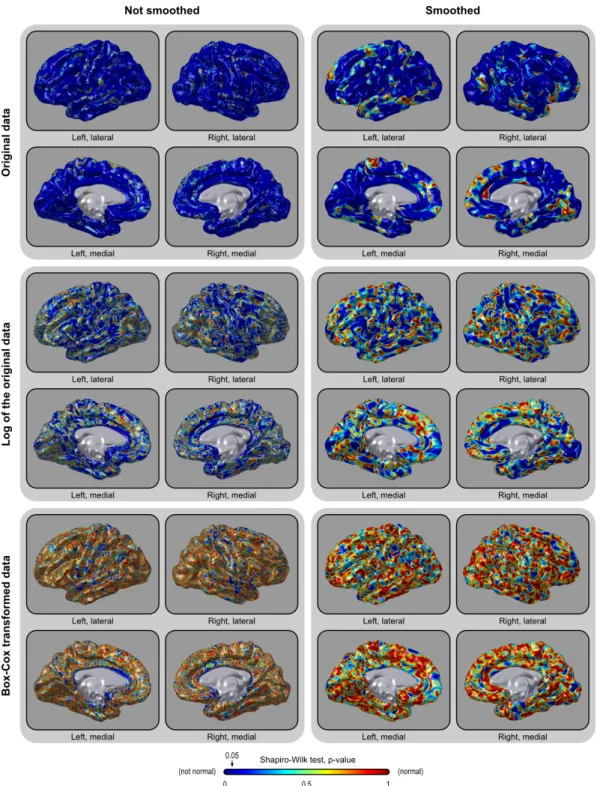
variance and are normally distributed. When these assumptions are not met, a non-linear transformation can be applied, as long as the true, biological or physical meaning that underlies the observed data is preserved. In the Evaluation section, we show empirically that facewise cortical surface area is largely not normal. In-stead, the distribution is skewed and can be better characterized as lognormal. A generic framework that can accommodate arbitrary areal quantities with skewed distributions is using a power transformation, such as the Box–Cox transformation (Box and Cox, 1964), which addresses possible violations of these specific assump-tions, allied with permutation methods for inference (Holmes et al., 1996; Nichols and Hayasaka, 2003, see also Chapter 3) when the observations can be treated as independent, such as in most between-subject analysis.

The application of a statistical test at each face allows the creation of a stat-istical map and also introduces the multiple testing problem, which can also be addressed using permutation methods. These methods are known to allow exact significance values to be computed, even when distributional assumptions can-not be guaranteed, and also to facilitate strong control over family-wise error rate (fwer) if the distribution of the statistic under the null hypothesis is similar across tests. If not similar, the result is still valid, yet conservative. An alternative is to use a relatively assumption-free approach to address multiple testing, controlling instead the false discovery rate (fdr) (Benjamini and Hochberg, 1995; Genovese et al., 2002), which offers also weak control over fwer. Other approaches for in-ference, such as the Random Field Theory (rft) for meshes (Worsley et al., 1999; Hagler et al., 2006) and the Threshold-Free Cluster Enhancement (tfce) (Smith and Nichols, 2009) have potential to be used.

(43)

2.3. Evaluation 41

2.2.11 Presentation of results

To display results, facewise data can be projected from the common grid to the template geometry, which helps to visually identify anatomical landmarks and name structures. Projecting data from one surface to another is trivial as there is a one-to-one mapping between faces of the grid and the template geometry. The statistics and associated p-values can be encoded in colors, and a color scale can be shown along with the surface model.

However, the presentation of facewise data has conceptual differences in com-parison with the presentation vertexwise data. For vertexwise data, each vertex cannot be directly colored, for being dimensionless. Instead, to display data per vertex, typically each face has its color interpolated according to the colors of its three defining vertices, forming a linear gradient that covers the whole face. For facewise data there is no need to perform such interpolation of colors, since the faces can be shown directly on the 3d space, each one in the uniform color that represents the underlying data. The difference is shown in Figure 2.6.

Interpolation of colors for vertexwise data should not be confused with the related, yet different concept of lightning and shading using interpolation. Both vertexwise and facewise data can be shaded to produce more realistic images. In Figure 2.6 we give an example of simple flat shading and shading based on linear interpolation of the lightning at each vertex (Gouraud, 1971).

Currently available software allow the presentation of color-encoded vertex-wise data on the surface of meshes. However, only very few software applications can handle a large number of colors per 3d object, being one color per face. One example is Blender (Blender Foundation, Amsterdam, The Netherlands), which we used to produce the figures presented in this chapter. Another option, for instance, is to use low-level mesh commands in matlab (The MathWorks Inc., 2015), such as “patch”.

2.3 Evaluation

We illustrate the method using data from the Genetics of Brain Structure and Func-tion Study, gobs, a collaborative effort involving the Texas Biomedical Institute,

(44)

Figure 2.6: Differences between presentation of facewise and vertexwise data can be ob-served in this zoomed portion of the mesh representation of the cortex. Vertices are di-mensionless and, to display vertexwise data, the faces have to be colored using linear interpolation. This is not necessary for facewise data, which can be shown directly in the uniform colors that represent the underlying data. In either case, the presentation can be improved by using a shading model, such as Gouraud in this example. Although the ver-texwise presentation may be visually more appealing, it contains only half the resolution of the facewise image.

(45)

the University of Texas Health Science Center at San Antonio (uthscsa) and the Yale University School of Medicine. The participants are members of 42 families, and total sample size, at the time of the selection for this study, is 868 subjects. We randomly chose 84 subjects (9.2%), with the sparseness of the selection minimiz-ing the possibility of drawminimiz-ing related individuals. The mean age of these subjects was 45.1 years, standard deviation 13.9, range 18.2–77.5, with 33 males and 51 females. All participants provided written informed consent on forms approved by each Institutional Review Board. The images were acquired using a Siemens magnetom Trio 3 T system (Siemens ag, Erlangen, Germany) for 46 participants, or a Siemens magnetom Trio/tim 3 T system for 38 participants. We used a T1

-weighted, mprage sequence with an adiabatic inversion contrast pulse with the following scan parameters: te/ti/tr = 3.04/785/2100 ms, flip angle = 13◦_{, voxel}

size (isotropic) = 0.8 mm. Each subject was scanned 7 (seven) times, consecutively, using the same protocol, and a single image was obtained by linearly coregistering these images and computing the average, allowing improvement over the signal-to-noise ratio, reduction of motion artifacts (Kochunov et al., 2006), and ensuring the generation of smooth, accurate meshes with no manual intervention. The im-age analysis followed the steps described in the Methods section, with some vari-ation to test different registrvari-ation strategies.

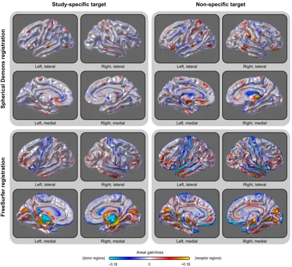
2.3.1 Registration

To isolate and evaluate the effect of registration, we computed the area per face after the spherical transformation⁶ and registered each subject brain hemisphere to a common target using two different registration methods, the Spherical Demons (Yeo et al., 2010a) and the FreeSurfer registration algorithm (Fischl et al., 1999b)⁷, each with and without a study-specific template as the target, resulting in four different variants. The study-specific targets for each of these methods were pro-duced using the respective algorithms for registration, using all the 84 subjects

⁶ Note that here the area was computed in the sphere with the aim of evaluating the registra-tion method. For analyses of areal quantities, these quantities should be defined in the native geometry, as previously described.

(46)

ing. This can be understood by observing that, as the vertices are shifted along the surface of the sphere, the faces that they define, and which carry areal quantities, are also shifted and distorted. The registration, therefore, causes displacement of areal quantities across the surface, which may accumulate on certain regions while other become depleted. Ideally, there should be no net accumulation when many subjects are considered and the target is unbiased with respect to the population under study. If pockets of accumulated or depleted areal quantities are present, this means that some regions are showing a tendency to systematically “receive” more areal quantities than others, which “donate” quantities. The average amount of area after the registration estimates this accumulation and, therefore, can be used as a measure of a specific kind of bias in the registration process, in which some regions consistently attract more vertices, resulting in these regions receiv-ing more quantities. The result for this analysis is shown in Figure 2.7. Usreceiv-ing default settings, sd caused less areal displacement across the surface, with less regional variation when compared to fs. The pattern was also more randomly dis-tributed for sd, without spatial trends matching anatomical features, whereas fs showed a structure more influenced by brain morphology. Using a study specific template further helped to reduce areal shifts and biases. The subsequent analyses we present are based on the sd registration with a study-specific template.

2.3.2 Distributional characterization

To evaluate the normality for the cortical area at the white surface of the nat-ive geometry, we used the Shapiro–Wilk normality test (Shapiro and Wilk, 1965), implemented with the approximations for samples larger than 50 as described by Royston (1993). The test was applied after each hemisphere of the brain was

(47)

re-2.3. Evaluation 45

Figure 2.7: A study-specific template (target for the registration) caused less systematic accumulation of areal quantities across the brain when compared with a non-specific tem-plate. Using default parameters, areal accumulation wa less pronounced and unrelated to sulcal patterns using Spherical Demons in comparison with FreeSurfer registration. Gains and losses refer to the area per face that would be expected for areal quantities being re-distributed with no bias, i.e. the zero corresponds to the average total surface area of all subjects, divided by the number of faces.

(48)

Cox transformation (Box and Cox, 1964). For a set of values y = {y1, y2, . . . , yn},

this transformation uses maximum-likelihood methods to seek a parameter λ that produces a transformed set ˜y ={˜y1, ˜y2, . . . , ˜yn} that approximately conforms to a

normal distribution. The transformation is a piecewise function given by:

˜ y =    yλ− 1 λ (λ̸= 0) ln y (λ = 0) (2.3)

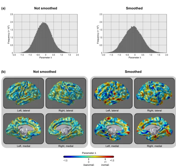
Not surprisingly, the Box–Cox transformation rendered the data more nor-mally distributed than a simple log-transformation. However, an interesting as-pect of this transformation is that the parameter λ is allowed to vary continu-ously, and it approaches unity when the data is normally distributed, and zero if lognormally distributed, serving, therefore, as a summary metric of how normally or lognormally distributed the data is. Throughout most of the brain, λ is close to zero, although with a relatively wide variation (mode =−0.057, mean = −0.099, sd = 0.493 for the analysed dataset), indicating that, at the resolution used, the white surface cortical area can be better characterized across the surface as a gradient of skewed distributions, with the lognormal being the most common case. The same was observed for facewise data smoothed in the sphere after interpolation with fwhm = 10 mm (mode =−0.142, mean = −0.080, sd = 0.578).⁸ Maps for the parameter λ are shown in Figure 2.14.

⁸ For scale comparison, the sphere has radius fixed and set as 100 mm, such that the Gaussian filter has an hwhm (half width) = 1.59% of the geodesic distance between the barycenter of any face and its antipode.

(49)

Figure 2.8: The area of the cortical surface is not normally distributed (upper panels). In-stead, it is lognormally distributed throughout most of the brain (middle panels). A Box– Cox transformation can further improve normality (lower panels). The same pattern is present without (left) or with (right) smoothing (fwhm = 10 mm). Although normality is not an assumption for inference as proposed, it offers some advantages, as discussed in the text.

(50)

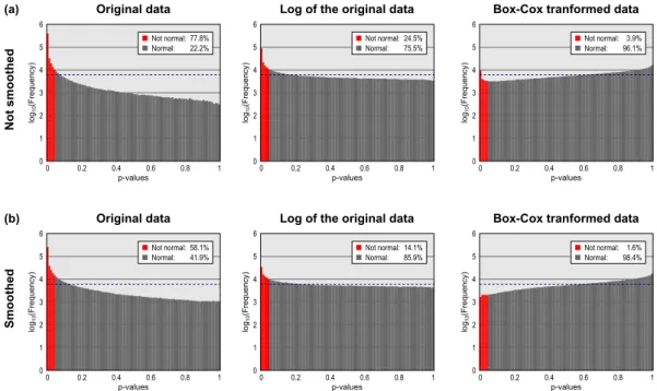
p-values 0 0.2 0.4 0.6 0.8 1 0 1 2 3 4 5 6 log 10 (Fre quency) Not normal: Normal: 58.1% 41.9% p-values 0 0.2 0.4 0.6 0.8 1 0 1 2 3 4 5 6 log 10 (Fre quency) Not normal: Normal: 1.6% 98.4% p-values 0 0.2 0.4 0.6 0.8 1 0 1 2 3 4 5 6 log 10 (Fre quency) Not normal: Normal: 14.1% 85.9% p-values 0 0.2 0.4 0.6 0.8 1 0 1 2 3 4 5 6 log 10 (Fre quency) Not normal: Normal: 24.5% 75.5% p-values 0 0.2 0.4 0.6 0.8 1 0 1 2 3 4 5 6 log 10 (Fre quency) Not normal: Normal: 3.9% 96.1% p-values 0 0.2 0.4 0.6 0.8 1 0 1 2 3 4 5 6 log 10 (Fre quency) Not normal: Normal: 77.8% 22.2%

Original data Log of the original data Box-Cox tranformed data

Not smoot

hed

Smooth

ed

Original data Log of the original data Box-Cox tranformed data (a)

(b)

Figure 2.9: Distribution of the uncorrected p-values of the Shapiro–Wilk normality test. For normally distributed data, 5% of these tests are always expected to be declared as not normal with a significance level of α = 0.05. Without transformation or smoothing, near 80% are found as not normal. Logarithmic and Box–Cox transformations render the data more normally distributed. Observe that the frequencies are shown in logscale. The dashed line (blue) is at the frequency that would be observed for uniformly distributed p-values.

(51)

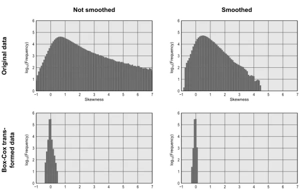
Figure 2.10: Maps of the skewness of the areal data, before and after the Box–Cox trans-formation, and with and without smoothing. The distribution is positively skewed (lognor-mal) throughout most of the brain, and the transformation successfully brings the data to symmetry (normality). The histograms are shown in Figure 2.11.

(52)

Skewness −1 0 1 2 3 4 5 6 7 log 10 (Fre quency) 0 1 2 3 4 6 5 Skewness −1 0 1 2 3 4 5 6 7 log 10 (Fre quency) 0 1 2 3 4 6 5 Skewness −1 0 1 2 3 4 5 6 7 log 10 (Fre quency) 0 1 2 3 4 6 5 Skewness −1 0 1 2 3 4 5 6 7 log 10 (Fre quency) 0 1 2 3 4 6 5

Not smoothed Smoothed

Original data

Box-C

ox

trans-formed dat

a

Figure 2.11: Histograms of the skewness of the areal data, before and after the Box–Cox transformation, and with and without smoothing. The distribution is positively skewed (lognormal) throughout most of the brain, and the transformation successfully brings the data to symmetry (normality). Note that the frequencies are shown in log scale. The corresponding maps are in Figure 2.10.

(53)

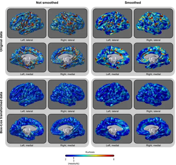
Figure 2.12: Maps of the kurtosis of the areal data, before and after the Box–Cox trans-formation, and with and without smoothing. The distribution is leptokurtic throughout most of the brain, and the transformation renders the kurtosis closer to the same value as for the normal distribution, i.e. closer to the value 3. The histograms are shown in Figure 2.13.