Analysis of Finite Word-Length Effects in Fixed-Point Systems

HAL Id: hal-01941888

https://hal.inria.fr/hal-01941888

Submitted on 4 Feb 2019

HAL is a multi-disciplinary open access

archive for the deposit and dissemination of

sci-entific research documents, whether they are

pub-lished or not. The documents may come from

teaching and research institutions in France or

abroad, or from public or private research centers.

L’archive ouverte pluridisciplinaire HAL, est

destinée au dépôt et à la diffusion de documents

scientifiques de niveau recherche, publiés ou non,

émanant des établissements d’enseignement et de

recherche français ou étrangers, des laboratoires

publics ou privés.

Analysis of Finite Word-Length Effects in Fixed-Point

Systems

Daniel Ménard, Gabriel Caffarena, Juan Antonio Lopez, David Novo, Olivier

Sentieys

To cite this version:

Daniel Ménard, Gabriel Caffarena, Juan Antonio Lopez, David Novo, Olivier Sentieys. Analysis of

Finite Word-Length Effects in Fixed-Point Systems. Shuvra S. Bhattacharyya. Handbook of Signal

Processing Systems, pp.1063-1101, 2019, 978-3-319-91733-7. �10.1007/978-3-319-91734-4_29�.

�hal-01941888�

Analysis of Finite Word-Length Effects in Fixed-Point Systems

D. Menard

, G. Caffarena

, J.A. Lopez

,

D. Novo

, O. Sentieys

February 4, 2019

Contents

1

Introduction

2

2

Background

4

2.1

Floating-Point vs. Fixed-Point Arithmetic . . . .

4

2.2

Finite Word-Length Effects . . . .

5

3

Effect of Signal Quantization

6

3.1

Error Metrics . . . .

7

3.2

Analytical Evaluation of the Round-Off Noise . . . .

7

3.2.1

Quantization Noise Bounds

. . . .

8

3.2.2

Round-Off Noise Power . . . .

12

3.2.3

Probability Density Function . . . .

15

3.3

Simulation-based and Mixed Approaches . . . .

16

3.3.1

Fixed-point Simulation-based Evaluation . . . .

16

3.3.2

Mixed Approach . . . .

17

4

Effect of Coefficient Quantization

18

4.1

Measurement Parameters . . . .

19

4.2

L

-Sensitivity . . . .

20

4.3

Analytical Approaches to Compute the L

-Sensitivity . . . .

21

5

System Stability due to Signal Quantization

22

5.1

Analysis of Limit Cycles in Digital Filters . . . .

23

5.2

Simulation-based LC Detection Procedures . . . .

24

∗_{Univ Rennes, INSA Rennes, IETR, Rennes, France} †_{University CEU-San Pablo, Madrid, Spain} ‡_{ETSIT, Universidad Polit´ecnica de Madrid, Spain}

§_{LIRMM, Universit´e de Montpellier, CNRS, Montpellier, France} ¶_{Univ Rennes, Inria, Rennes, France}

6

Summary

24

Abstract

Systems based on fixed-point arithmetic, when carefully designed, seem to behave as their infinite precision analogues. Most often, however, this is only a macroscopic impression: finite word-lengths inevitably approximate the reference behavior introducing quantization errors, and confine the macroscopic correspondence to a restricted range of input values. Understanding these differences is crucial to design optimized fixed-point implementations that will behave “as expected” upon deployment. Thus, in this chapter, we survey the main approaches proposed in literature to model the impact of finite precision in fixed-point systems. In particular, we focus on the rounding errors introduced after reducing the number of least-significant bits in signals and coefficients during the so-called quantization process.

1

Introduction

The use of fixed-point (FxP) arithmetic is widespread in computing systems. Demanding appli-cations often force computing systems to specialize their hardware and software architectures to reach the required levels of efficiency (in terms of energy consumption, execution speed, etc.). In such cases, the use of fixed-point arithmetic is usually not negotiable. Yet, the cost benefits of fixed-point arithmetic are not for free and can only be reached through an elaborated design methodology able to restrain finite word-length – or quantization – effects.

Digital systems are invariably subject to nonidealities derived from their finite precision arith-metic. A digital operator (e.g., an adder or a multiplier) imposes a limited number of bits (i.e., word-length) upon its inputs and outputs. As a result, the values produced by such an operator suffer from (small) deviations with respect to the values produced by its “equivalent” (infinite precision) mathematical operation (e.g., the addition or the multiplication). The more the bits allocated the smaller the deviation – or quantization error – but also the larger, the slower and the more energy hungry the operator. The so-called word-length optimization – or quantization – process determines the word-length of every signal (and corresponding operations) in a tar-geted algorithm. Accordingly, the best possible quantization process needs to select the set of word-lengths leading to the cheapest implementation while bounding the precision loss to a level that is tolerable by the application in hand. The latter can formally be defined as the following optimization problem:

minimize

w C(w)

subject to D(w) ≤ Ω,

(1)

where w is a vector containing the word-lengths of every signal, C(·) is a cost function that propa-gates variations in word-lengths to design objectives such as energy consumption, D(·) computes the degradation in precision caused by a particular w and Ω represents the maximum precision loss tolerable by the application.

From a methodological perspective, the word-length optimization process can be approached in two consecutive steps: (1) range selection and (2) precision optimization. The range selection step defines the left hand limit – or Most-Significant Bit (MSB) – and the subsequent precision optimizationstep fixes the right hand limit – or Least-Significant Bit (LSB) – of each word-length. Typically, the range selection step is designed to avoid overflow errors altogether, and therefore, the precision optimization step becomes the sole responsible for precision loss. Figure 1 gives a pictorial impression of the word-length optimization process and divides the precision optimiza-tion step into four interacting components, namely the optimizaoptimiza-tion engine, the cost estimaoptimiza-tion, the constraint selection and the error estimation.

• The optimization engine basically consists of an algorithm that iteratively converges to the best word-length assignment. It has been shown that the constraint space is non-convex in

Optimization engine Cost estimation Error estimation Precision constraint Word-lengths Error Cost Constraint selection Range selection Precision optimization LSB1...LSBS MSB1...MSBS Signal1 Signal2 SignalS MSB1 LSB1 MSB2 LSB2 MSBS LSBS ... Binary point

Figure 1: Basic components of a word-length optimizaton process

nature [29] – it is actually possible to have a lower quantization error at a system output by reducing the word-length at an internal node –, and that the optimization problem is NP-hard [35]. Accordingly, existing practical approaches are of a heuristic nature [32, 21, 22]. • A precise cost estimation of each word-length assignment hypothesis leads to impractical

optimization times as such heuristic optimization algorithms involve a great number of cost and error evaluations. Instead, word-length optimization processes use fast abstract cost models, such as the hardware cost library introduced in the chapter [132] of this book or the fast models proposed by Clarke et al. [28] to estimate the power consumed in the arithmetic components and routing wires.

• The precision constraint selection block is responsible of reducing the abstract sentence “the maximum precision loss tolerable by the application” into a magnitude that can be measured by the error estimation. Practical examples have been proposed for audio [103] or wireless applications [109].

• Existing approaches for error estimation can be divided into simulation-based and analytical methods. Simulation-based methods are suitable for any type of application but are gener-ally very slow. Alternatively, analytical error estimation methods can be significantly faster but often restrict the domain of application (e.g., only linear time-invariant systems [32]). There are also hybrid methods [122] that aim at combining the benefits of each method. While the chapter presented in [132] covers in breadth most of the blocks in Figure 1, this chapter takes a complementary in-depth approach and focuses on arguably the most important block in the word-length optimization process: the error estimation. The latter is crucial to ensure correctly behaving fixed-point systems and has received considerable attention in the research literature. Thus, in this chapter, we survey the main approaches proposed to model quantization errors. To understand their similarities and differences, we present a classification of the reviewed approaches based on their assumptions and coverage. We believe that this chapter will shed some light on the word-length optimization process as a whole and help readers choose the most conve-nient available approach to model quantization errors in their word-length optimization process.

The rest of the chapter is organized as follows. Section 2 introduces the main concepts re-garding quantization. The next section deals with signal quantization. Noise metrics and both simulation-based and analytical techniques for the evaluation of quantization noise are explained. Regarding the analytical evaluation, this covers both the estimation of noise power and noise bound. Section 4 addresses the quantization of coefficients. The different meausurement param-eters used to evaluate coefficient quantization are explained, with special enphasis on the use of the L2-sensitivity. System stability is described in section 5, again focusing on simulation-based

and analytical approaches. Finally, a summary is presented in the last section.

Specification Implementation Algorithmic refinement Bit-true optimizations Accuracy refinement Algebraic approximation Static data formatting ideal operators and signals real operators real operators and signals Algorithmic approximation i.e., Accurate operations and signals i.e., Accurate signals

but limited accuracy operators (e.g., divide by zero)

Bit-true specification

Figure 2: Basic DSP design flow

2

Background

A typical Digital Signal Processing (DSP) design flow begins with a design specification and follows a number of steps to produce a satisfactory implementation as illustrated in Figure 2. The original specification serves as a functional reference and is typically implemented in frame-works that prioritize software productivity, such as MATLAB, in floating-point or double pre-cision. For instance to illustrate, such a specification can include a 64-point Discrete Fourier Transform (DFT). Firstly, a skillful designer will reduce the algorithmic complexity in the algo-rithmic refinement step. The DFT matrix can be factorized into products of sparse factors (i.e., Fast Fourier Transform), which reduces the complexity fromO(n2) toO(nlogn). Additionally, the algorithmic refinement step can make use of approximations to further reduce the complex-ity – e.g., the Maximum Likelihood (ML) detector is approximated by a near-ML detector [109]. Once the algorithm structure is fixed, operators and signals are defined in the subsequent alge-braic transformationand static data formatting steps, respectively. An algebraic approximation can for instance reduce a reciprocal square root operator to a scaled linear function [109]. Finally, the static data formatting step is the responsible of finalizing the bit-true specification that will constrain all succeeding (bit-true) optimizations, such as loop transformations, resource binding, scheduling, etc.

Algorithmic and algebraic approximations are integrating parts of what is known as approx-imate computing[107]. Instead, data formatting is equivalent to the word-length optimization process introduced in the previous section. Although some prior work targets implementations that do not add quantization error to those of the inputs [9, 130, 84], lossy static data format-ting [34] – i.e., reduction of implementation cost by introducing additional quantization noise in intermediate nodes – is the common practice and the main focus of this chapter.

2.1

Floating-Point vs. Fixed-Point Arithmetic

The IEEE-754 standard [60] for floating-point (FlP) arithmetic – particularly the 64 bit double-precision format – is commonly used in implementations requiring high mathematical double-precision. However, many applications tolerate the use of less precise arithmetic modules in both FxP [34,

120] and non-standard FlP [51] formats. As introduced in Chapter [132], the FlP format represents numbers by means of two variables: an exponent e and a mantissa m. Given the pair (m, e), the value of the represented FlP number, V_FlP, is

VFlP= m · 2e. (2)

The combined use of mantissa and exponent provides the finest level of scaling: each number includes its own scaling factor. Thereby, FlP digital systems can effectively operate numbers with a very wide dynamic range. However, FlP arithmetic often involves overheads in terms of area, delay and energy consumption. Firstly, FlP requires wider bit-widths than FxP arithmetic to operate with equivalent precision on variables with low to moderate dynamic range [57], which is the typical case in most applications. Furthermore, FlP operators are more complex as they implement in hardware the alignment of the fractional point of the operands and the normalization of the output besides the actual operator.

Alternatively, FxP arithmetic constrains the exponent e to be a design time constant. Equa-tion (2) remains valid but only the mantissa m changes at run time – and thus needs to be stored in memory. Accordingly, describing an implementation employing FxP arithmetic is more complex and tedious as the designer is responsible of handling explicitly in the source code the scaling of variables.

2.2

Finite Word-Length Effects

Quantized systems suffer from two types of errors: overflow and precision errors. On the one hand, overflow errors result from variable values growing beyond the limits of the word-length. They are related to the lack of scaling and saturation and wrap-around [119, 97, 116] are the most common techniques used to handle them at the operator output. Saturation employs extra hardware to detect and reduce overflow error. Instead, wrap-around is hardware-free but leads to intolerably huge errors in underdimensioned word-lengths. On the other hand, precision errors are due to the unavoidable limited precision of quantized digital implementations [119, 97, 116]. Rounding and truncation are the most common techniques used to handle precision errors at the operator output. Rounding employs extra hardware to reduce the maximum error magnitude re-sulting from the removal of LSBs. Instead, truncation is hardware-free but often accumulates larger precision errors. The technique leading to the most implementation is application depen-dent: even though rounding requires more complex operators, they can generally operate shorter word-lengths to achieve the same precision error as truncation [98].

The limited precision effects of the DSP realizations have been studied extensively since the raise of digital systems, particularly in Linear Time Invariant (LTI) systems [119, 97, 116]. They are commonly divided in four different types: round-off noise, coefficient quantization, limit cy-cles and system stability. Round-Off Noise (RON) refers to the probabilistic deviation of the results of a quantized implementation with respect to the error-free reference [119, 97, 116]. Coefficient Quantization (CQ) refers to the deterministic deviation of the parameters of the transfer func-tion [71, 119, 97]. Limit Cycles (LC) are the parasitic oscillafunc-tions that appear in quantized system under constant or zero inputs due to the propagation of the quantization errors through feedback loops [27, 119]. Finally, in the case of digital filters, the coefficient quantization modifies the position of the poles of the transfer function, which might jeopardize the system stability when approached carelessly [110]. Table 1 summarizes the classification of these effects attending to linearity and whether they result from the quantization of signals or coefficients.

RON is the prominent finite precision effect during normal operation of FxP systems [71, 119, 97, 116]. It introduces stochastic variations around the system’s nominal operation point. Complementary, CQ effects modify the actual nominal operation point of the system and can lead to instability when such deviation is not carefully conducted. While RON and CQ effects apply to any FxP system, LCs effects are only relevant to particular types of systems (e.g., DSP filters) as they are the result of correlated quantization errors in feedback loops [119, 116]. For this reason,

Table 1: Classification of the finite WL quantization effects

Type of effect

Quantization object

Name of effect

Linear

Signals

Round-Off Noise (RON)

(Section III)

Coefficients

Coefficient Quantization (CQ)

(Section IV)

Nonlinear

Signals

Limit Cycle Oscillations

Coefficients

System Instability

in this chapter we focus mainly on RON (most of Section 3) and CQ effects (Section 4) while also covering LCs for the sake of completeness but in much less detail (end of Section 3).

3

Effect of Signal Quantization

Finite precision arithmetic leads to unavoidable deviations of the finite precision values from the infinite precision ones. Such deviations, due to signal quantizations, modify the quality of the ap-plication output. Thus, they must be evaluated and maintained within reasonable bounds. In most cases these deviations are accurately modeled as additive white noise, or quantization noise. The quantization noise can be evaluated through analytical or fixed-point simulation based approaches. In the case of analytical approaches, a mathematical expression of a metric is determined. Com-puting an expression of an quality metric for every kind of application is generally an issue. Thus, the quality degradations are not analyzed directly in the quantization process, but an intermediate metric measuring the fixed-point accuracy is used instead.

Word-length optimization is split into two main steps. Firstly, a computational accuracy con-straint is determined according to application quality and, secondly, the word-length optimization is carried out using this constraint. Interestingly, fixed-point simulation approaches enable the direct evaluation of the effect of quantization on application quality. But, in many cases, an in-termediate accuracy metric is used because less samples are required to estimate this metric in contrast to directly computing or simulating application quality under quantization effects.

The different approaches available to analyze quantization noise effects that are covered in this section are displayed in Fig. 3. The techniques are first divided into the three main major groups: simulation-based, analytical and mixed (that combines the two previous ones) approaches. The graph include all techniques covered in the subsequent subsections and also the main related publications.

Fig. 4 shows the main classification of systems used by the different techniques devoted to RON evaluation: LTI systems, smooth systems and all systems. Smooth systems are those whose operations are differentiable and can be linearized without commiting a significant error. This classification also distinguishes between recursive systems – systems with loops or cyclic – and non-recursive systems – systems without loops or acyclic. The different regions displayed in the graph are related to different techniques that are only able to handle a particular type of systems.

Section 3.1 introduces the different noise metrics used. Section 3.2 covers the analytical evaluation of the quantization noise effect, embracing both the noise power and noise bound

Analysis of quantization effects Simulation based approaches Optimized Fixed-point Data Types Hardware Emulation [78, 73, 39, 82, 37, 38] Bit-level Mapping optimization [39, 82, 76, 36, 143] Object-Oriented Data Types [75, 96, 11, 104, 77] Mixed approaches Application Quality Metric Mixed approach [113] Analytical approaches

Figure 3: Classification of the different approaches to analyze the quantization noise effects

computation. Then the techniques based on fixed-point simulation and the hybrid techniques are presented in Section 3.3.

3.1

Error Metrics

Different metrics can be used to measure the accuracy of a fixed-point realization. This accuracy can be evaluated through the bounds of the quantization errors [43, 2], the number of significant bits [24], or the power of the quantization noise [102, 126, 18]. The shape of the power spectral density (PSD) of the quantization noise is used as metric in [7] or in [31] for the case of digital filters. In [20], a more complex metric able to handle several models is proposed.

Regarding the metric that computes the bounds of the quantization errors, the maximum devi-ation between the exact value and the finite precision value is determined. This metric is used for critical systems when it is necesary to ensure that the error will not surpass a maximum deviation. In this case, the final quality has to be numerically validated.

As for the noise power computation, the error is modeled as a noise, and the second order moment is computed. This metric analyzes the dispersion of the finite precision values around the exact value and the mean behaviour of the error. The noise power metric is used in applications which tolerate sporadic high-value errors that do not affect the overall quality. In this case, the system design is based on a trade-off between application quality and implementation cost.

3.2

Analytical Evaluation of the Round-Off Noise

The aim of analytical approaches is to determine a mathematical expression of the fixed-point error metric. The error metric function depends on the word-length of the different data inside the

Figure 4: Classification of systems targeted by RON evaluation techniques

Analytical approaches Error Power Metric Perturbation Theory Hybrid Approach [126, 33, 56] Impulse Response Deter-mination [100, 122], AA-based Simulation [18, 93] Probability Density function Metric Unsmooth [127, 115] Smooth Karhunen-Loeve Expansion (KLE) [145, 3] Polynomial Chaos Expansion (PCE) [146, 50] Error Bound Metric Interval Arithmetic (IA) [23, 5], [45, 41, 124] Affine Arithmetic (AA)[52], [95, 86, 93], [111, 13] Multi-IA (MIA) [94, 1, 80, 81]

Figure 5: Classification of the different analytical approaches to analyze the quantization noise effects

application. The main advantage of these approaches is the short time required for the evaluation of the accuracy metric for a given set of word-lengths. The time required to generate this analytical function can be more or less important but this process is done only once, before the optimization process. Then, each evaluation of the accuracy metric for a given WL sets corresponds to the computation of a mathematical expression. The main drawback of these analytical approaches is that they do not support all kinds of systems. Figure 5 depicts a classification of existing analytical approaches to analyze the quantization noise effects. This classification depends on the type of metric used (bound, power or probability density function), on the smooth/unsmooth nature of the noise, and on the technique used. In this section, we review the different analytical approaches for computing: RON bounds, RON power, and the effect of RON on any quality metric in the presence of unsmooth operators.

3.2.1

Quantization Noise Bounds

There are a number of techniques and methods that have been suggested in the literature to mea-sure the bounds of the quantization noise. Since the numerical techniques typically lead to exceed-ingly long computation times, different alternatives have been proposed to obtain results faster.

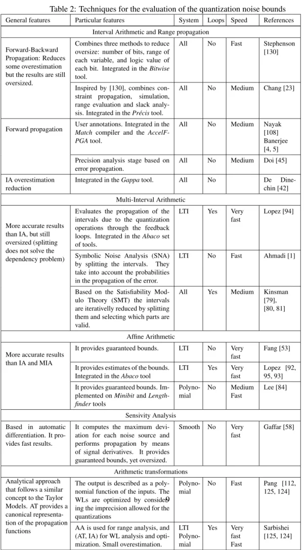
Table 2 shows the most relevant techniques related to the evaluation of noise bounds. The first column indicates the name of the technique. The second column displays the main characteristics of the technique, while the third column shows particular features of the cited approaches. The next three columns contain information about the type of systems that the approaches can be applied to (all, polynomial, based on smooth operations and LTI systems), the existence of loops and the computational speed of the approach.

The analytical techniques used to evaluate the noise bounds can be classified in two major groups: (i) interval-based computation (Interval Arithmetic (IA), Multi-IA (MIA), Affine Arith-metic (AA) and satisfiability modulo theory) and (ii) polynomial representation with interval re-mainders (sensitivity analysis and Arithmetic Transformations (AT)). Principal techniques are described in the following paragraphs.

Interval-based computations

In the last decade, interval-based computations have emerged as an alternative to simulation-based techniques. A high number of simulations are required in order to cover a significant set of possible values of the inputs, so traditional simulation-based techniques imply very long computation times. As an alternative, interval-based methods have been suggested to speedup

Table 2: Techniques for the evaluation of the quantization noise bounds

General features Particular features System Loops Speed References

Interval Arithmetic and Range propagation Forward-Backward

Propagation: Reduces some overestimation but the results are still oversized.

Combines three methods to reduce oversize: number of bits, range of each variable, and logic value of each bit. Integrated in the Bitwise tool.

All No Fast Stephenson

[130]

Inspired by [130], combines con-straint propagation, simulation, range evaluation and slack analy-sis. Integrated in the Pr´ecis tool.

All No Medium Chang [23]

Forward propagation User annotations. Integrated in the Match compiler and the AccelF-PGAtool.

All No Medium Nayak

[108] Banerjee [4, 5] Precision analysis stage based on

error propagation.

All No Medium Doi [45]

IA overestimation reduction

Integrated in the Gappa tool. All No De

Dine-chin [42] Multi-Interval Arithmetic

More accurate results than IA, but still oversized (splitting does not solve the dependency problem)

Evaluates the propagation of the intervals due to the quantization operations through the feedback loops. Integrated in the Abaco set of tools.

LTI Yes Very

fast

Lopez [94]

Symbolic Noise Analysis (SNA) by splitting the intervals. They take into account the probabilities in the propagation of the error.

LTI No Fast Ahmadi [1]

Based on the Satisfiability Mod-ulo Theory (SMT) the intervals are iterativelly reduced by splitting them and selecting which parts are valid.

All Yes Medium Kinsman

[79], [80, 81]

Affine Arithmetic More accurate results

than IA and MIA

It provides guaranteed bounds. LTI No Very fast

Fang [53] It provides estimates of the bounds.

Integrated in the Abaco tool

LTI Yes Very

fast

Lopez [92, 95, 93] It provides guaranteed bounds.

Im-plemented on Minibit and Length-findertools Polyno-mial No Medium Fast Lee [84] Sensivity Analysis Based in automatic differentiation. It pro-vides fast results.

It computes the maximum devi-ation for each noise source and performs propagation by means of signal derivatives. It provides guaranteed bounds, yet oversized.

Smooth No Very

fast

Gaffar [58]

Arithmetic transformations Analytical approach

that follows a similar concept to the Taylor Models. AT provides a canonical representa-tion of the propagarepresenta-tion functions

The output is described as a poly-nomial function of the inputs. The WLs are optimized by consider-ing the imprecision allowed for the quantizations

Polyno-mial

No Fast Pang [112,

125, 124]

AA is used for range analysis, and (AT, IA) for WL analysis and opti-mization. Small overestimation.

LTI Polyno-mial Yes Very fast Fast Sarbishei [125, 124]

9

the computation process. The results are obtained much faster, but they have to deal with the continuous growth of the intervals (oversizing) through the sequence of operations. Thus, these techniques are restricted to a limited subset of systems (mostly LTI or quasi-LTI), or combined with other techniques to reduce the oversize.

The most classical approach is the computation using interval arithmetic (IA), also called forward propagation, value propagation or range propagation techniques. Given the ranges of the inputs of a system, represented by intervals, IA computes the guaranteed ranges of the outputs. The main drawback of these techniques is the so-called dependency problem, which is produced when the same variable is used in several places within the algorithms under analysis, since IA is not able to track dependency between variables, ranges are overestimated. To alleviate this situation, some authors have suggested splitting the intervals in a number of sections, generating a Multi-IA approach.

One of the earliest work that applied value propagation to the computation of the noise bounds was developed by Stephenson et al. in the Bitwise project [130]. They perform forward and backward range propagation, and combine three different types of analysis to optimize the WLs with guaranteed accuracy: analysis of the number of bits, the ranges of the operands, and the logic value of each bit. The analysis of the number of bits provides larger WLs than the analysis of ranges, but limits the LSB of the result. In combination with backward propagation, the evaluation of the logic values of the operands enables some optimization, but it is not significant in the general case. Since the oversizing of these techniques rapidly increases along the sequence of operations, this approach does not provide practical results in complex systems. However, it provides fast and guaranteed results for smaller blocks.

Chang et al. have applied a similar approach in the Pr´ecis tool [23]. By including fixed-point annotations in Matlab code, they perform fixed-fixed-point simulation, range analysis, forward and backward propagation, and slack analysis. The annotations are based on the routine fixp, which allows modelling different integer and fractional WLs, as well as overflow and underflow quantization strategies. They indicate that the combined application of range analysis (MSB) and propagation analysis (LSB) provides accurate WLs, and that the propagation based on the number of bits is more conservative than range analysis for the MSBs. Slack analysis uses the difference between these two results to provide an ordered list of signals that provide better results when their LSBs are optimized [23].

Nayak [108] and Banerjee et al., [4, 5] have applied the propagation techniques to the compu-tation of the noise bounds. They have developed an automatic quantization environment that has been included in the Match project and the AccelFPGA tool.

In [45], Doi et al., present a WL optimization method that estimates the optimum WLs using noise propagation. They propagate the noise ranges using IA, and apply it in combination with a nonlinear programming solver to estimate the optimum WLs in LTI blocks without loops. Due to the oversizing of the interval-based computations, the bounds provided in this process are conservative in most cases, but the difference with the optimum result is not significant in blocks without loops.

The Gappa tool [42, 41] uses a different approach to deal with the oversizing associated to the interval computations. It creates a set of theorems to rewrite the most common expressions into similar ones that are less affected by the correlations in the interval computations. This approach provides guaranteed and accurate results, but up to now its application is limited to systems without loops and branches [41], and requires a very good knowledge of the target system [42].

Multi-IA(MIA) has also been applied by several authors to reduce the width of the bounds of the quantization noise. In [94], the authors suggest a method to reduce the overestimation of IA and use it to provide refined bounds in the impulse response and the transfer function of an IIR filter. Although MIA provides less conservative bounds than IA, MIA does not solve the dependency problem and is therefore not a good option for systems with loops [95].

The Symbolic Noise Analysis (SNA) method presented in [1] splits the noise intervals into smaller parts and performs IA propagation of each part. At the output, intervals are combined

according to their probabilities to provide the histogram of the output noise. When there is small or no oversizing, this approach provides accurate estimates of the PDF of the output noise. However, in the general case, this only provides bounds associated to each part, and less conservative global bounds than IA or range propagation methods.

Kinsman and Nicolici [80, 81] propose to use Satisfiability Modulo Theory (SMT). This ap-proach initially performs IA propagation of the values of all the signals and noise sources, and provides an initial (conservative) estimate of the bounds at the output. After that, all the sources are successively split using the bisection method to provide less conservative ranges in each iter-ation. The process finishes after reaching a given constraint or when all the intervals have zero width (degenerated intervals). The authors indicate that this method is particularly useful in pres-ence of discontinuities (such as in systems with divisions or inverse functions) and that it provides more accurate results than AA in non-linear systems [79]. In later work, the authors have general-ized this idea to handle floating- and fixed-point descriptions using the same solver [80] and have introduced vectors to reduce the amount of terms in the splitting process [81].

Affine Arithmetic(AA) [131] was proposed to optimize the bounds of signals and noise sources in LTI fixed-point realizations [53]. The authors propose to apply AA for feed-forward systems to obtain guaranteed bounds and also to obtain a practical estimation based on a confidence interval. Moreover, an iterative method is proposed for systems with feedback and is proved to always converge although the bounds are overestimated. A more detailed analysis about the application of AA to characterize quantized LTI systems has been carried out in [92, 95, 93]. The authors have evaluated the source and propagation models of AA in fixed-point LTI systems with feedback loops, and have concluded that AA propagates the exact results in systems described by sequences of affine operations (i.e., LTI systems). In [92] and [95], they propose a variation of the description of the quantization operations of AA that provides more accurate estimates of the noise bounds. A comparison between IA, MIA, AA and the proposed approach shows that IA and MIA are affected by the dependency problem in most LTI systems with feedback loops (whenever the filter has complex poles), and do not provide useful results [95]. In [93], the expressions for the generation of the affine sources, the propagation of the noise terms, and the computation of the output results are provided. Although they are oriented to the computation of the MSE statistics, the derivation of the corresponding expressions to obtain the minimum guaranteed bounds is very easily obtained.

AA has also been suggested in combination with Adaptive Simulated Annealing (ASA) to perform WL optimization of fixed-point systems without feedback loops in the tool Minibit [85]. Polynomial representations with interval remainders

The polynomial representations with interval remainders are based on the perturbation theory and follow a similar idea to the Taylor Models. They perform a polynomial Taylor series decom-position and the smallest uncertainties can be merged in one or more terms, or simply they can be neglected. These approaches have been suggested, in particular in recent years, to perform efficient evaluation of polynomial sequences of operations.

Perturbation theory is based on a Taylor series decomposition of a given order and can include intervals to provide guaranteed bounds of the results. This idea was first presented by Wadekar and Parker [140], but the implementation details of the computation were not given. The most relevant contributions are those based on sensitivity analysis (using first-order derivatives) and arithmetic transformations (canonical polynomial representations with an error interval remainder). Handel-man representations [12] can handle more detailed representations of the internal descriptions, they are out of the scope of this paper since their application so far is to floating-point systems.

Gaffar et al. [58] have suggested an approach based on an automatic differentiation method and have applied it to linear or quasi-linear systems. The noise bounds are computed as the sum of the maximum deviation of each noise signal multiplied by its corresponding sensitivity. The main advantage of this approach is that the bounding expression is very easily obtained, since in this type of systems the sensitivities are the operands of the multiplications and the other terms of the Taylor series are considered negligible. However, since it is aimed at providing guaranteed

i i  0  0 j j

+

+

Figure 6: Model for the computation of output RON power based on noise sources b

and gains α

bounds of the results, the provided WLs are usually overestimated even for small blocks [58]. Another interesting approach which acquired relevance in the latest years is the optimization of systems using Arithmetic Transformations (AT) [112, 125, 124]. ATs are polynomials that rep-resent pseudo-boolean functions. Their extensions also include word-level inputs and sequential variables in the representations. AT representations are canonical, so the propagation of the poly-nomial terms is guaranteed to be accurate. In addition, due to their origin, they are particularly well suited to describe and optimize the operations of a given circuit.

In [112], authors distinguish three sources of error: approximation by the finite-order poly-nomial, quantization of the input signals, and optimization of the WLs of coefficients and result [112]. The combination of these three sources must be less than the specified error bound to provide a valid implementation. They initially determine the order of the Taylor series and the amount of input quantization. After that, a branch and bound algorithm, tuned for this applica-tion and guided by the sensitivity, is used for the optimizaapplica-tion process [112]. In [125] and [124], the authors extend this approach to evaluate systems containing feedback loops. In [125], they provide the analytical expressions for the analysis of IIR filters, taking into account both MSE statistics and bounds as the target measurements. In [124], they extend this analysis to polyno-mial systems with loops, and show that AT paired with IA is more efficient than AA to provide the noise bounds. One of the main features of this approach is that it does not require numerical simulations, unlike other similar approaches.

3.2.2

Round-Off Noise Power

Existing approaches to compute the analytical expression of the quantization noise power are based on perturbation theory, which models finite precision values as the addition of the infinite precision values and a small perturbation. At node i, a quantization error signal biis generated

when some bits are eliminated during a fixed-point format conversion (quantization). This error is assimilated to an additive noise which propagates inside the system. This noise source contributes to the output quantization noise bythrough the gain αi, as shown in Fig. 6.

The aim of this approach is to define the output noise bypower expression according to the

noise source biparameters and the gains αibetween the output and a noise source.

Table 3 summarizes the main techniques to compute the RON power. The first column indi-cates the type of technique used. The second column displays the main characteristic of the tech-nique, while the next column shows particular features of the cited approaches. The next three columns contain information about the type of systems that the approches handle (All, based on smoothoperations and LTI), the existance of loops and the computational speed of the approach. The last columns shows the references to the published works.

The next paragraphs focus on the model used for the quantization process, which has three phases: (i) noise generation, (ii) noise propagation, and (iii) noise aggregation.

Noise Generation

In finite precision arithmetic, signal quantization leads to an unavoidable error. A commonly used model for the continuous-amplitude signal quantization has been proposed in [141] and refined in [129]. The quantization of signal x is modeled by the sum of this signal and a random variable b (quantization noise). This additive noise b is a uniformly distributed white noise that is uncorrelated with signal x and any other quantization noise present in the system (due to the quantization of other signals). The validity conditions of the quantization noise properties have been defined in [129]. These conditions are based on characteristic function of the signal x, which is the Fourier transform of the probability density function (PDF). This model is valid when the dynamic range of signal x is sufficiently greater than the quantum step size and the signal bandwidth is large enough.

Table 3: Techniques for the analytical evaluation of the quantization noise power

Hybrid Techniques Based on statistical expressions. Requires large matrix computations.

Coefficients Kiand Li jare

computed using fixed-point simulations and then subtituted in the statistical matrix equations.

Smooth Yes Medium Shi [126] Smooth Yes Medium Constantinides

[33] Smooth Yes Medium Fiore [56] Impulse Response Determination

Based on system transformations. Provides fast results.

Coefficients Kiand Li jare

computed from the impulse response between the noise sources and the output. Integrated in the ID.Fix tool.

LTI Yes Very

fast

Menard [100] Smooth Yes Fast Rocher [122]

Affine Arithmetic Simulations Based on AA

simulations. Provides fast results.

Coefficients Kiand Li jare

computed from the results of the AA simulations. Integrated in the Abaco and Quasar tools.

LTI Yes Very

fast

Lopez [93]

Smooth Yes see

note1

Caffarena[18]

Combines MAA and PCE.

Provides accurate results in strongly nonlinear systems.

Poly-nomial Yes Medium/ Fast Esteban [50] 1_{: Fast for}

LTI & non-linear acyclic systems and slow for non-linear cyclic systems

This model has been extended to include the computation noise in a system resulting from some bit elimination during a fixed-point format conversion. More especially, the round-off error resulting from the multiplication of a constant by a discrete amplitude signal has been studied in [6]. This study is based on the assumption that the PDF is continuous. However, this hypothesis is no longer valid when the number k of bits eliminated during a quantization operation is small. Thus, in [30], a model based on a discrete PDF is suggested and the first and second-order mo-ments of the quantization noise are given. In this study, the probability value of each eliminated bit to be equal to 0 or 1 is assumed to be 1/2.

Noise Propagation

Each noise source bipropagates to the system output and contributes to the noise byat the output.

The propagation noise model is based on the assumption that the quantization noise is sufficiently small compared to the signal to consider that the finite precision values can be modeled by using the addition of the infinite precision values and a small perturbation. A first-order Taylor

imation [33, 121] is used to linearize the operation behavior around the infinite precision values. This approach allows obtaining a time-varying linear expression of the output noise according to the input noise [99]. In [126], a second-order Taylor approximation is used directly on the expression of the output quantization noise. In [93] and [18], affine arithmetic is used to model the propagation of the quantization noise inside the system. Affine expression allows obtaining directly a linear expression of the output noise according to the input noises. For non-affine op-erations, a first order Taylor approximation is used to obtain a linear behaviour. These models, based on the perturbation theory, are only valid for smooth operations. An operation is considered to be smooth if the output is a continuous and differentiable function of its inputs.

Noise Aggregation

Finally, the output noise byis the sum of all the noise source contributions. The second order

moment of bycan be expressed as a weighted sum of the statistical parameters of the noise source:

E(b2_y) = Ne

∑

∑

∑

bi are respectively the mean and the variance of noise source bi, and Ne is the

total number of error sources. These terms depends on the fixed-point formats and are determined during the evaluation of the accuracy analytical expression. The terms Ki and Li j are constant

and depend on the computation graph between biand the output. Thus, these terms are computed

only once for the evaluation of the accuracy analytical expression. These constant terms can be considered as the gain between the noise source and the output.

For the case of Linear Time-Invariant systems, the expressions of Kiand Li jare given in [101].

The coefficient Li jcan now be computed by the multiplication of terms Liand Lj, which can be

calculated independently. The coefficients Kiand Li jare determined from the transfer function

Hi(z) or the impulse response hi(n) of the system having bias input and byas output. In [102, 100],

a technique is proposed to compute these coefficients from the SFG (Signal Flow Graph) of the application. The recurrent equation of the output contribution of bi is computed by traversing

the SFG representing the application at the noise level. To support recursive systems, for which the SFG contains cycles, this SFG is transformed into several Directed Acyclic Graphs (DAG). The recurrent equations associated to each DAG are computed and then merge together after a set of variable substitutions. The different transfer functions are determined from the recurrent equations by applying a Z transform.

In [18], AA is used to keep track of the propagation of every single noise contribution along the datapath, and from this information the coefficients Kiand Liare extracted. The method has

been proposed for LTI in [93] and for non-LTI systems in [18]. An affine form, defined by a central value and an uncertainty term (error term in this context), is assigned to each noise source. These terms depend on the mean and variance of the noise source. Then, the central value and the uncertainty terms associated to each noise source are propagated inside the system through an affine arithmetic based simulation. The values of the coefficients Kiand Liiare extracted from

the affine form of the output noise. In the case of recursive systems, it is necessary to use a large number of iterations to ensure that the results converge to stable values. In some cases, this may lead to large AA error terms and therefore to long computation time.

In the method proposed in [122], an analytical expression of the coefficients Ki and Li j is

determined. For each noise source bi, the recurrent equation of the output contribution of bi

is determined automatically from the application SFG with the technique presented in [100]. A time-varying impulse response hiis computed from each recurrent equation. The output

quantiza-tion noise byis the sum of the noise source biconvolved with its associated time varying impulse

response. The second-order moment of byis determined. The expression of the coefficients is

proposed in [122]. These coefficients can be computed directly from their expression by approx-imating an infinite sum, or a linear prediction approach can be used to obtain more quickly the value of these coefficients. The statistical parameters of the signal terms involved in the

expres-sion of the coefficients are computed from a single floating-point simulation, leading to reduced computation times. The analysis to compute coefficients Kiand Li jis done on an SFG

represent-ing the application and where the control flow has been removed. To avoid loop unrollrepresent-ing which can lead to huge graph, a method based on polyhedral analysis has been proposed in [44].

Different hybrid techniques [126, 33, 56] that combine simulations and analytical expressions have been proposed to compute the coefficients Kiand Li j from a set of simulations. In [126],

these Ne(Ne+ 1) coefficients are obtained by solving a linear system in which Kiand Li jare the

variables. The way to proceed is to carry out several fixed-point simulations where a range of val-ues for σbiand µbi is covered for each noise source. The fixed-point parameters of the system are

set carefully to control each quantizer and to analyze its influence on the output. For each simula-tion, the statistical parameters of each noise source biare known from the fixed-point parameter

and the output noise power is measured. At least Ne(Ne+ 1) fixed-point simulations are required

to be able to solve the system of linear equations. A similar approach is used in [56] to obtain the coefficients by simulation. Each quantizer is perturbed to analyze its influence at the output to determine Kiand Lii. To obtain the coefficients Li jwith i 6= j, the quantizers are perturbed in

pairs. This approach requires again Ne(Ne+ 1) simulations to compute the coefficients, which

requires long computation times.

During the last fifteen years, numerous work on analytical approaches for RON power esti-mation have been conducted and interesting progresses have been made for the autoesti-mation of this process. These approaches allow for the evaluation of the RON power and are very fast compared to simulation-based approaches. Theoretical concepts have been established enabling the devel-opment of automatic tools to generate the expression of the RON power. The limit of the proposed methods have been identified. Analytical approaches based on perturbation theory are valid for systems made-up of only smooth operations.

3.2.3

Probability Density Function

The probability density function (PDF) of the quantization noise has been used as a metric to ana-lyze the effect of signal quantization. This metric provides more information than the quantization error bounds or the quantization noise power. They are of special interest if applied to the analysis of unsmooth operations since error bounds or noise power are mainly suitable for differentiable operations.

There are two types of measures used to optimize quantized systems: statistical analysis of the quantization noise, and guaranteed bounds of the results. In most cases, statistical analysis tech-niques only compute the mean and variance of the quantization noise (or, alternatively, the noise power) at the output signal. Since the number of noise sources is usually high, these techniques assume that the Central Limit Theorem is valid, and the output noise follows a Gaussian distri-bution. Consequently, these two parameters fully characterize the distribution of the quantization noise. However, in systems with non-linear blocks (such as slicers) the Central Limit Theorem can no longer be valid, and a more detailed analysis is required. In this sense, some work focused on evaluating the PDF of the quantization noise.

In the context of guaranteed bounds, the objective is to ensure that the maximum distortion in-troduced in the quantization process is below a given constraint. Some techniques select the WLs and perform the computations to ensure that the bounds of the quantization noise are below this constraint. Other techniques focus on ensuring that the output of the quantized system is equal to a valid reference (e.g., the floating-point one). In both cases, to obtain efficient implementations, it is important to ensure that the provided bounds are close to the numerical ones, and that the oversizing included in the process (if any) is small.

Stochastic approaches, based on Karhunen-Lo`eve Expansion (KLE) and Polynomial Chaos Expansion (PCE), have been used to model the quantization noise at the output of a system. The output quantization noise PDF can be extracted from the coefficients of the KLE or PCE. In the domain of fixed-point system design, these techniques have been previously proposed to

Figure 7: Simulation-based computation of quantization error

determine the signal dynamic range in LTI [145] and non-LTI systems [146]. In [3], a stochastic approach using KLE is used to determine the quantization noise PDF of an LTI system output. The KLE coefficients associated to a noise source are propagated to the output by means of the impulse response between the noise source and the system output. In [50], a stochastic approach based on a combination of Modified Affine Arithmetic (MAA) and Polynomial Chaos Expansion (PCE) is proposed to determine the output quantization noise PDF. Compared to KLE based approach, PCE allows supporting non-LTI systems. This technique is based on decomposing the random variables into weighted sums of Legendre orthogonal polynomials. The Legendre polynomial bases are well suited to represent uniformly distributed random variables, thus, they are very efficient to model quantization noise.

The determination of the PDF is required to handle unsmooth operations. In [127], the effect of quantization noise on the signum function is analyzed. This work has been extended in [115] to handle more complex decision operations which have specific contours like in QAM (Quadrature Amplitude Modulation) constellation diagrams. These two models are defined for one single unsmooth operation. Handling systems with several unsmooth operations is still an open issue for purely analytical approaches.

3.3

Simulation-based and Mixed Approaches

3.3.1

Fixed-point Simulation-based Evaluation

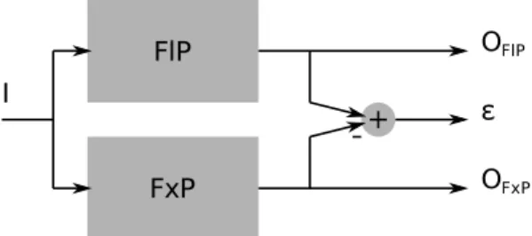
The quantization error can be obtained by extracting the difference between the outputs of sim-ulation when the system has a very large precision (e.g. simsim-ulation with double-precision floating-point) and when there is quantization (bit-true fixed-point simulation), as shown in Fig. 7. Floating-point simulation is considered to be the reference given that the associated error is definitely much smaller than the error associated to fixed-point computation. Different error metrics can be computed from the quantization error obtained from this simulation. The main advantage of simulation-based approaches is that every kind of application can be supported. Fixed-point simulation can be performed using tools such as [40, 75, 96, 47].

Different C++ classes, to emulate the fixed-point mechanisms have been proposed, such as sc fixed(SystemC) [11], ac fixed (Algorithm C Data Types) [104] or gFix [77]. The C++ class attributes define the fixed-point parameters associated to the data: integer and fractional word-lengths, overflow and quantization modes, signed/unsigned operations. For ac fixed, the fixed-point attributes can be parametrized through template parameters. For sc fixed, these attributes can be static to obtain fast simulations or dynamic so they can be modified at run-time. Bit-true operations are performed by overloading the different arithmetic operators. During the execution of a fixed-point operation, the data range is analyzed and the overflow mode is applied if required. Then, the data is cast with the appropriate quantization mode. Thus, for a single fixed-point operation, several processing steps are required to obtain a bit true simulation. Therefore, these techniques suffer from a major drawback which is the extremely long simulation time [39]. This becomes a severe limitation when these methods are used in the data word-length optimiza-tion process where multiple simulaoptimiza-tions are needed. The simulaoptimiza-tions are made on floating-point

machines and the extra-code used to emulate fixed-point mechanisms increases the execution time between one to two orders of magnitude compared to traditional simulations with native floating-point data types [76, 36]. Besides, to obtain an accurate estimation of the statistical parameters of the quantization error, a great number of samples must be taken for the simulation. This large number of samples combined with the fixed-point mechanism emulation lead to very long simu-lation time.

Different techniques have been proposed to reduce this overhead. The execution time of the fixed-point simulation can be reduced by using more efficient fixed-point data types. In [77], the aim is to reduce the execution time of the fixed-point simulation by using efficiently the floating-point units of the host computer. The mantissa is used to compute the integer operations. Thus, the word-length of the data is limited to 53 bits for double data types. The execution time is one order of magnitude greater than the one required for a fixed-point simulation. This technique is also used in SystemC [11] for the fast fixed-point data types.

The fixed-point simulation can be accelerated by executing it on a more adequate machine like a fixed-point DSP [78, 73, 39, 82, 37] or an FPGA [38] through hardware acceleration. In the case of hardware implementation, the operator word-length, the supplementary elements for overflow and quantization modes are adjusted to comply exactly with the fixed-point specification which has to be simulated. In the case of software implementation, the operator and register word-lengths are fixed. When the word-length of the fixed-point data is lower than the data word-length supported by the target machine, different degrees of freedom are available to map the fixed-point data into the target storage elements. In [39], to optimize this mapping, the execution time of the fixed-point simulation is minimized. The cost integrates the data alignment and the overflow and quantization mechanism. This combinatorial optimization problem is solved by a divide and conquer technique and several heuristics to limit the search space are used. In [82] a technique is proposed to minimize the execution time due to scaling operations according to the shift capa-bilities of the target architecture. In the same way, the aim of the Hybris simulator [76] [36] is to optimize the mapping of the fixed-point data described with SystemC into the target architecture register. All compile-time information are used to minimize the number of operations required to carry-out the fixed-point simulation. The overflow and quantization operations are implemented by conditional structures, a set of shift operations or bit mask operations. Nevertheless, to obtain fast simulation, some quantization modes are not supported. In [143], the binary point alignment is formulated as a combinatorial optimization problem and an integer linear programming ap-proach is used to solve it. But, this apap-proach is limited to simple applications to obtain reasonable optimization times. These methods reduce the execution time of the fixed-point simulation but, this optimization needs to be performed every time that the fixed point configuration changes. Accordingly, it might not compensate for the execution time gain of the fixed-point simulation when involving complex optimizations.

3.3.2

Mixed Approach

To handle systems made-up of unsmooth operations, a mixed approach which combines analyti-cal evaluations and simulations has been proposed in [113, 114]. The idea is to evaluate directly the application performance metric with fixed-point simulation and to accelerate drastically the simulation with analytical models. In this technique the analytical approach is based on the per-turbation theory and the simulation is used when the assumptions associated with perper-turbation theory are no longer valid (i.e. when a decision error occurs). In this case, the quantization noise at the unsmooth operation input can modify the decision at the operation output compared to the one obtained with infinite precision.

This technique selectively simulates parts of the system only when an decision error occurs [114]. Given that decision errors are rare event the simulation time is not so important as for classical fixed-point simulations. The global system is divided into smooth clusters made-up of smooth operations. These smooth clusters are separated by unsmooth operations. The single

source noise model [103] is used to capture the statistical behavior of quantization noise accu-rately at the output of each smooth cluster. In [103], The authors propose to model the output quantization noise of a LTI system with a weighted sum of a Gaussian random variable and a uni-form random variable. In [123], the output quantization noise of a smooth system is modeled by a generalized Gaussian random variable, whose parameters define the shape of the PDF. These pa-rameters are analytically determined from the output quantization noise statistics (mean, variance and kurtosis). The general expression of the noise moments are given in [123], and are computed from the impulse responses between the noise sources and the system output.

4

Effect of Coefficient Quantization

Coefficient Quantization (CQ) is the part of the implementation process that describes the degra-dation of the system operation due to the finite WL representation of the constant values of a system. Especially this problematic is of high importance for LTI systems with the quantization of the coefficients. Opposite to RON, CQ modifies the impulse and frequency responses for LTI system and the functionality for other systems. In the analysis of the quantization effects for LTI systems, this parameter is the first to be determined, since it involves two major tasks: (i) the selection of the most convenient filter structure to perform the required operation, and (ii) the determination of the actual values of the coefficients associated to it.

Figure 8 illustrates the amount of deviation due to CQ by means of interval simulations. A butterworth filter has been realized in DFIIt (Direct Form II transposed) form, and each coefficient has been replaced by a small interval that describes the difference between the ideal coefficient and the quantized one using 7 fractional bits. Figure 8.a shows the impulse response of the real-ization, where the size of each interval reveals how sensitive is each sample to this quantization of coefficients. Figure 8.b shows the transfer function associated to it, where in this case the intervals reveal the most sensitive frequencies to the same set of quantizations.

(a) (b)

Figure 8: Effect of CQ on a given filter realization: (a) Evolution in time of the impulse response

of the differences in the output response. (b) Distribution of the effects in the frequency domain.

The intervals represent the deviation between the quantized and unquantized samples of the impulse

response and the transfer function.

In LTI systems, CQ has been traditionally measured using the so-called Coefficient Sensi-tivity (CS). Although this parameter was originally defined for LTI systems, whose operation is described by H(z), its current use has also been extended to non-linear systems.

Table 4 summarizes the most important techniques and groups related to the computation of the CS. The first column indicates the type of technique used to compute this parameter (residues,

geometric sum of matrices, Lyapunov equations, perturbation theory). The second and third columns respectively provide the most important work in this area, and the most relevant fea-tures in each case. The last two columns provide the main advantages and disadvantages of the different approaches. First, an overview of the different parameters used in the literature to measure the CS is presented, before discussing in more detail the L2-sensitivity. Second, the most

commonly-used L2-sensitivity computation procedures are described. Finally, a generic algorithm

that perform fast computation of the L2-sensitivity is described.

Table 4: Measurement techniques for the computation of the Coefficient Sensitivity (CS)

Features Advantages Disadvantages References

Evaluation of the Residues General analytical procedure

based on complex mathematical equality.

General method. Provides exact results.

Very complex to de-velop. Different anal-ysis for each struc-ture.

Roberts [119]

Geometric Sum of Matrices Analytical procedure that

ap-proximates SL12by using infinite

sums in state-space realizations.

The analytical expres-sionis easier to obtain.

Limited to state-space realizations. Provides an upper bound. Hinamoto [66] Lyapunov Equations Provides the analytical

expres-sion for families of filter struc-tures, mainly state-space realiza-tions.

Fast and exact re-sults (without infinite sums).

Iterative method. Limited to certain fil-ter structures. Li [89] Hilaire [64] Perturbation Theory Compute the sum of deviations of all the coefficients. Analytical ap-proach based on Lyapunov Equa-tion.

Extremely fast, if the analytical expression is obtained Limited to state-space realizations. Xiao [147] Interval-based pro-cedure.

Fast and automatic. Valid for all types of systems. Approximated value. Requires interval computations sup-port. Lopez [91]

4.1

Measurement Parameters

A number of procedures have been initially suggested to minimize the degradation of H(z) with respect to the quantization of all coefficients of the realization under different constraints [133, 134, 135]. In these procedures, the coefficients of the realization have been obtained by minimiz-ing the so-called L1/L2-sensitivity, SL12 [133, 134, 135, 69, 59, 144, 68, 67]. The main feature

of this parameter is that its upper bound is easily obtained [59, 144, 88]. However, two different norms are applied to obtain the result. Therefore, its physical interpretation is not clear.

Instead, it is more natural to measure the deviations of H(z) using only the L2-norm [68, 88].

For this reason, the so-called L2-sensitivity, SL2, is currently applied [68, 67]. The main feature

of this parameter is that it is proportional to the variance of the deviation of H(z) due to the quantization of all the coefficients of the realization [59, 144, 68, 67]. However, the computa-tion of its analytical expression requires performing extremely complex mathematical operacomputa-tions [144, 68, 89]. Due to this fact the computation of the L2-sensitivity has been limited to simple

linear structures, typically SSR (State-Space Representation) forms. Since each analytical expres-sion only characterizes one family of filter structures, it requires developing a new mathematical expression to optimize or compare each new structure. The most recent work in this area are focused on minimizing the L2-sensitivity of two-dimensional (2-D) SSR filter structures [68, 67],

and of structures based on the generalized delta operator [89, 148].

In [136, 137, 138], the authors have compared the performance of the filter structures by computing the maximum value of the magnitude sensitivity, Smag, or the relative sensitivity, Smag.

The main feature of Smag and Srel is that their numerical values are more easily computed than

the analytical expressions of SL12 or SL2. For this reason, they have been used in combination

with simulated annealing or genetic algorithms that perform automated search of the most robust structures against the quantization of coefficients [136, 137, 138]. However, Smag and Srel only

provide information of the maximum deviations of H(z). In contrast, the L2-sensitivity provides

global information about the deviations of H(z). For this reason, this parameter is widely preferred [59, 68, 88, 89, 66].

In [64], the authors introduce a unified algebraic description able to represent the most widely used families of filter realizations. They focus on the fixed- and floating-point deviation of the transfer function and pole measures using CS parameters. They apply Adaptive Simulated An-nealing to obtain the optimal realization among these structures. In particular, they introduce the SW_L2measure, which considers the individual quantization of coefficients into the traditional L2-sensitivity parameter. This work has been further expanded in [62] to include L2-scaling

con-straints, and in [63] to include the evaluation of MIMO filters and controllers.

Table 5 summarizes the parameters introduced in this Section. In each column, the representa-tion of the different parameters, the main references associated to them, and their most important features, advantages and disadvantages are also briefly outlined.

Table 5: Measurement parameters for coefficient quantization

Parameter Features Advantages Disadvantages References

SL12 Initial measure of the

coef-ficient sensitivity,

based on the L1and the L2

-norms. It has a sim-ple expression in some filter structures Only provides an upper bound, based on two different norms.

[133, 134, 135, 69]

SL2 Advanced measurement,

based only on the L2-norm.

Development of the expres-sions associated to each filter structure. Global measure-ment. It has statistical meaning. Complex to de-velop. [59, 144, 68, 67, 88, 89, 148]

Smag, Srel Information about the

mag-nitude of the quantizations.

Computationally simple. Only provides information about the maximum deviations. [136, 137, 138]

SW_L2 Measures the actual devi-ations of coefficients with different amount of quanti-zations. More accurate than SL2. Requires com-plex analytical developments. [64, 62, 63]

4.2

L

-Sensitivity

Since the L2-Sensitivity is much more commonly used than the others CQ measurement

parame-ters, in this section its mathematical definition and physical interpretation are described in more detail.