Asymptotic analysis for the multiscale modeling of defects in mechanical structures

HAL Id: hal-01516460

https://hal.archives-ouvertes.fr/hal-01516460

HAL is a multi-disciplinary open access

archive for the deposit and dissemination of sci-entific research documents, whether they are pub-lished or not. The documents may come from teaching and research institutions in France or abroad, or from public or private research centers.

L’archive ouverte pluridisciplinaire HAL, est destinée au dépôt et à la diffusion de documents scientifiques de niveau recherche, publiés ou non, émanant des établissements d’enseignement et de recherche français ou étrangers, des laboratoires publics ou privés.

Public Domain

Asymptotic analysis for the multiscale modeling of

defects in mechanical structures

Eduard Marenic, Delphine Brancherie, Marc Bonnet

To cite this version:

Eduard Marenic, Delphine Brancherie, Marc Bonnet. Asymptotic analysis for the multiscale modeling of defects in mechanical structures. 12e Colloque national en calcul des structures, CSMA, May 2015, Giens, France. �hal-01516460�

CSMA 2015

12e Colloque National en Calcul des Structures 18-22 Mai 2015, Presqu’île de Giens (Var)

Asymptotic analysis for the multiscale modeling of defects in

mechan-ical structures

E. Mareni´c1, D. Brancherie1, M. Bonnet2

1_{Laboratoire Roberval, Université de Compiegne, {eduard.marenic, delphine.brancherie}@utc.fr} 2_{POems, ENSTA, Palaiseau, mbonnet@ensta.fr}

Abstract — This research is a first step towards designing a numerical strategy capable of assessing the nocivity of a small defect in terms of its size and position in the structure with low computational cost, using only a mesh of the defect-free reference structure. The proposed strategy aims at taking into account the modification induced by the presence of a small defect through displacement field correction using an asymptotic analysis. Such an approach would allow to assess the criticality of defects by introducing trial micro-defects with varying positions, sizes and mechanical properties.

Key words — defect, asymptotic analysis, elastic moment tensor.

1

Introduction

The role played by defects in the initiation and development of rupture is crucial and has to be taken into account in order to realistically describe the behavior till complete failure. The difficulties in that context revolve around (i) the fact that the defect length scale is much smaller than the structure length scale, and (ii) the random nature of their position and size. Even in a purely deterministic approach, taking those defects into consideration by standard models imposes to resort to geometrical discretisations at the defect scale, leading to very costly computations and hindering parametric studies in terms of defect location and characteristics.

Our current goal is to design an efficient two-scale numerical strategy which can accurately predict the perturbation (in terms of displacement or stress concentration) caused by an inhomogeneity in elastic (background) material given by elasticity tensor (C). To make it computationally efficient, the analysis uses only a mesh for the defect-free structure, i.e. the mesh size does not depend on the (small) defect scale. The latter is instead taken into account by means of a multiscale asymptotic expansion (see e.g. [1, 2]), in which the concept of elastic moment tensor (EMT) [3, 4] plays an important role.

2

Problem definition

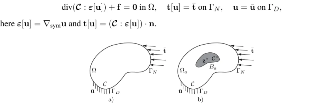
We consider an elastic body occupying a smooth bounded domain Ω ⊂ R3 characterized by elasticity tensor C. The background solution in terms of displacement field u arising in the reference solid Ω due to prescribed excitation (f , ¯t, ¯u), is defined by the problem

div(C : ε[u]) + f = 0 in Ω, t[u] = ¯t on ΓN, u = ¯u on ΓD, (1)

where ε[u] = ∇symu and t[u] = (C : ε[u]) · n.

Figure 1: Model scheme showing the unperturbed a) and perturbed b) domains, Ω and Ωa, respectively. The

The transmission problem for a small trial inhomogeneity involves a small elastic (C?) inhomogene-ity located at z ∈ Ω, of characteristic linear size a, occupying the domain Ba:= z+aB, where B ⊂ R3is

a smooth fixed domain centered at the origin and defines the inhomogeneity shape. The elastic properties of the whole solid are defined as

C_a:= Cχ_Ω\Ba+ C?χBa, (2)

where χDis the characteristic function of a domain D. Material contrast, or elastic tensor perturbation, is

given by ∆C = C?−C. The displacement field uaarising in the solid containing the small inhomogeneity

due to prescribed excitation (f , ¯t, ¯u), solves the transmission problem

(a) div(Ca: ε[ua]) + f = 0 in Ω, (b) t[ua] = ¯t on ΓN, (c) u = ¯uaon ΓD. (3)

(where the perfect-bonding transmission conditions are implicitly enforced via (3a) written in the distri-butional sense and the usual smoothness assumption ua∈ H1(Ω)).

Furthermore, let the displacement perturbation va := ua− u be given as the difference of the total

and unperturbed displacement. Two distinct asymptotic expansions of va arise, namely a near-field

expansion and a far-field expansion. The near-field expansion is given by

va(x) = avB(¯x) + o(a), (4)

where ¯x := (x − z)/a are coordinates at the defect scale and vBis the solution (in terms of displacement

perturbation) of the auxiliary problem of a perfectly bonded inhomogeneity B embedded in an infinite elastic medium and subjected to the constant remote stress C : ∇u(x). Such solutions vB are known

analytically for simple inhomogeneity shapes (in which case they correspond to the famous Eshelby inclusion problem), see [5]. Expansion (4) is valid for finite ¯x, i.e. within a neighbourhood of Bawhose

linear size is O(a).

The far field expansion is given by

va(x) = −∇G(z, x) : A(B, C, ∆C) : ∇u(z)a3+ o(a3), x 6= z, (5)

where G(z, x) denotes Green’s tensor for the domain Ω, and A(B, C, ∆C) is the elastic moment tensor (EMT), both entities being described thereafter. In this work, as a first step, we only address the compu-tation of the far-field approximation (5), which is valid at a finite (independent on a) distance from the inhomogeneity.

Elastostatic Green’s tensor and elastic moment tensor. The quantities in (5) are now briefly intro-duced. Starting with the elastostatic Green’s tensor G(ξ, x) which is defined as a solution of

div(C : ε[G(·, x)]) + δ(· − x)I = 0 in Ω, t[G(·, x)] = 0 on ΓN, G(·, x) = 0 on ΓD. (6)

The Green’s tensor gathers the three linearly independent elastostatic displacement fields Gk(·, x) re-sulting from unit point forces δ(· − x)ek applied at x ∈ Ω along direction k. We further introduce a

decomposition of G as

G(·, x) = G∞(· − x) + Gc(·, x), (7)

where G∞is the singular, infinite-space Green’s tensor, such that

div(C : ε[G∞]) + δI = 0 in R3, |G∞(ξ − x)| → 0 as |ξ − x| → ∞, (8)

and the complementary Green’s tensor Gcis bounded at ξ = x and represents a correction of G∞due

to the finite size of Ω. More precisely, by a superposition argument, Gcsolves the elastostatic

boundary-value problem (BVP) with regular boundary data and zero body force density:

div(C : ε[∇Gc]) = 0, ∇Gc= −∇G∞on ΓD, t[∇Gc] = −t[∇G∞] on ΓN, (9)

where the boundary data is related to the trace of ∇G∞ on ∂Ω, treated columnwise as displacement

fields, and the traction vectors associated with those displacements. Note that problem (9) in fact involves 9 loading cases for 3D conditions (and 4 for 2D conditions).

We continue with the EMT, which as shown in e.g. [4] is the key mathematical concept in the asymp-totic expansion of va, and is also involved for formulating accurate effective elastic properties of

compos-ite materials. The EMT carries important microstructural information, namely the material contrast ∆C, the inhomogeneity shape B and its orientation (see e.g. Definition 2.3. in [3] for details and properties of the EMT). We focus here on the EMT A associated with an ellipsoidal inhomogeneity (B, C + ∆C) embedded in a medium with elasticity tensor C, which is given by [3]

A = |B|C : (C + ∆C : S)−1: ∆C, (10)

where S = S(B, C) denotes the (fourth-order) Eshelby tensor of the normalized inclusion B [5]. We now focus on the special case of plane strain, corresponding to an ellipsoidal inclusion B infinitely elongated in the x3direction, assuming C and C? to be both isotropic. In this case, the nonzero components of the

Eshelby tensor S are given explicitly as

S1111 = A(1 − m)(3 + γ + m), S1122 = A(1 − m)(1 − γ − m),

S2222 = A(1 − m)(3 + γ − m), S2211 = A(1 + m)(1 − γ + m), (11)

S1212 = A(1 + m2+ γ),

where A = 1/[8(1 − ν)], γ = 2(1 − 2ν), and m = (a1− a2)/(a1 + a2), with a1and a2 denoting the

semi-axes of the ellipse B in principal directions x1and x2, respectively (while a3 → ∞).

3

Computational steps and numerical example

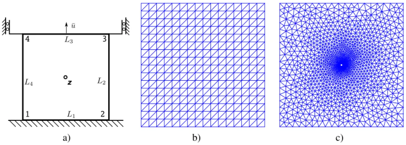
The capabilities of the proposed strategy are illustrated on a preliminary and academic example involving the uniaxial stretch of a membrane clamped on its upper and lower edges (Fig. 2a). The steps of the proposed strategy for accurate evaluation of the perturbation caused by an inhomogeneity are as follows. We first compute the background solution u defined by (1) using a coarse mesh (Fig. 2b). The goal is, as described above, to correct this unperturbed solution using (5) in order to achieve results comparable with the reference solution performed on a fine mesh (Fig. 2c).

Next, for a inhomogeneity with given location, shape and properties (z ∈ Ω, B, C?), we extract the gradient of the background displacement ∇u(z) and compute the EMT A(B, C, ∆C) using (10).

Having these results in hand, we then proceed to the calculation of the gradient of the Green’s tensor ∇G = ∇G∞+ ∇Gc. The part ∇G∞ is a simple derivative of the textbook fundamental solution

(usually called Kelvin solution), see e.g. [6]. The complementary part ∇Gcis then computed numerically

by solving problem (9).

All the required ingredients for evaluating the far-field asymptotic approximation (5) of vaare now

available, and that solution may afterwards be post-processed for evaluating the defect criticality.

z

1 2

3 4

a) b) c)

Figure 2: Scheme of the geometry and boundary conditions of the uniaxial stretch of the membrane clamped on upper and lower edges a). The position of the inhomogeneity is given with z. FE mesh of unperturbed, background b) and reference models c). Unperturbed consists of 289, and reference of 2346 nodes.

58E+00 1 2 E+00 3 1 E 01 3 1 E 01 1 2 E+00 58E+00 9 E+00 9 E+00 DISPLACEMENT Time = 0 00E+00 4 93E+00 3 94E+00 2 96E+00 1 97E+00 9 85E 01 0 00E+00 9 85E 01 1 97E+00 2 96E+00 3 94E+00 4 93E+00 5 91E+00 5 91E+00 DISPLACEMENT 1 Time = 0 00E+00

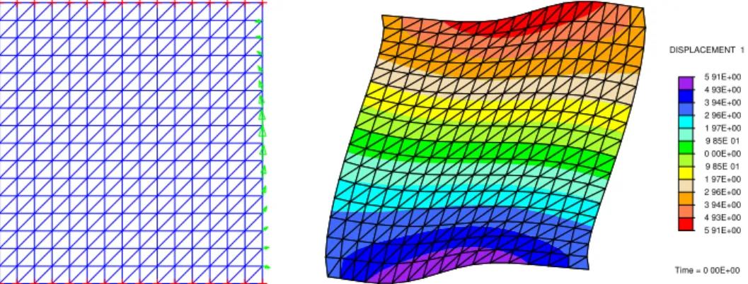
Figure 3: Mesh and BCss used to solve (9) (left). The upper and lower edges are Dirichlet boundaries, the others being Neumman boundaries. The corresponding solution (component 1) is shown on the right with a large amplification factor.

4

Conclusion and perspectives

A numerical strategy for predicting the perturbation caused by an inhomogeneity in an elastic solid is outlined. We focus on the evaluation of the far field displacement correction. Thanks to the use of an asymptotic expansion, the defect scale is not meshed. The computations involved are straightforward. Special attention is given to the computation of the complementary part of Green’s tensor, i.e. the direct calculation of its gradient and the correct imposition of the BC’s, a step that also does not require any meshing at the defect scale.

The next steps of this work include (i) matching the near and far-field asymptotic expansions to obtain uniform expansions, and (ii) applying the developed strategy to assessing the criticality of defects by considering virtual micro-defects and varying their positions, sizes and mechanical properties.

Acknowledgement. The authors are funded by ANR through project ARAMIS (ANR 12 BS01-0021).

References

[1] D. Brancherie, M. Dambrine, G. Vial, and P. Villon. Effect of surface defects on structure failure: a two-scale approach. Eur. J. Comput. Mech., 17:613–624, 2008.

[2] M. Dambrine and G. Vial. A multiscale correction method for local singular perturbations of the boundary. ESAIM: Mathematical Modelling and Numerical Analysis, 41(1):111–127, 2007.

[3] M. Bonnet and G. Delgado. The topological derivative in anisotropic elasticity. Quart. J. Mech. Appl. Math., 66:557–586, 2013.

[4] H. Ammari. Polarization and moment tensors. With applications to inverse problems and effective medium theory. Springer-Verlag, New York, Applied Mathematical Sciences Series Vol. 162s, 2007.

[5] T. Mura. Micromechanics of Defects in Solids. Martinus Nijhoff Publishers, 1987.