HAL Id: hal-00428967
https://hal.archives-ouvertes.fr/hal-00428967
Submitted on 30 Oct 2009
HAL is a multi-disciplinary open access
archive for the deposit and dissemination of
sci-entific research documents, whether they are
pub-lished or not. The documents may come from
teaching and research institutions in France or
L’archive ouverte pluridisciplinaire HAL, est
destinée au dépôt et à la diffusion de documents
scientifiques de niveau recherche, publiés ou non,
émanant des établissements d’enseignement et de
recherche français ou étrangers, des laboratoires
A Constraint on the Number of Distinct Vectors with
Application to Localization
Gilles Chabert, Luc Jaulin, Xavier Lorca
To cite this version:
Gilles Chabert, Luc Jaulin, Xavier Lorca. A Constraint on the Number of Distinct Vectors with
Application to Localization. CP’09 (15th International Conference on Principles and Practice of
Constraint Programming), Sep 2009, Lisbon, Portugal. p. 196-210. �hal-00428967�
A Constraint on the Number of Distinct Vectors
with Application to Localization
Gilles Chabert1, Luc Jaulin2, and Xavier Lorca1 1 Ecole des Mines de Nantes LINA CNRS UMR 6241,
4, rue Alfred Kastler 44300 Nantes, France
gilles.chabert@emn.fr xavier.lorca@emn.fr
2 ENSIETA, 2, rue Fran¸cois Verny 29806 Brest Cedex 9, France
luc.jaulin@ensieta.fr
Abstract. This paper introduces a generalization of the nvalue con-straint that bounds the number of distinct values taken by a set of vari-ables.The generalized constraint (called nvector) bounds the number of distinct (multi-dimensional) vectors. The first contribution of this paper is to show that this global constraint has a significant role to play with continuous domains, by taking the example of simultaneous localization and map building (SLAM). This type of problem arises in the context of mobile robotics. The second contribution is to prove that enforcing bound consistency on this constraint is NP-complete. A simple contrac-tor (or propagacontrac-tor) is proposed and applied on a real application.
1
Introduction
This paper can be viewed as a follow-up of [7] on the application side and [1] on the theoretical side. It proposes a generalization of the nvalue global constraint in the context of a relevant application. The nvalue constraint is satisfied for a set of variables x(1),. . ., x(k) and an extra variable n if the cardinality of
{x(1), . . . , x(k)} (i.e., the number of distinct values) equals to n. This constraint
appears in problems where the number of resources have to be restricted. The generalization is called nvector and matches exactly the same definition, except that the x(i)are vectors of variables instead of single variables. Of course, all the
x(i)must have the same dimension (i.e., the same number of components) and the constraint is that the cardinality of {x(1), . . . , x(k)} must be equal to n.
We first show that this new global constraint allows a much better modeling of the SLAM (simultaneous localization and map building) problem in mobile robotics. In fact, it allows to make automatic and thus robust a process part of which was performed by hand. Second, we classify the underlying theoretical complexity of the constraint. Finally, a simple algorithm is given and illustrated on a real example.
Since the application context involves continuous domains, we shall soon focus on the continuous case although the definition of nvector does not depend on
the underlying type of domains.
The application is described in Section 2. We first give an informal description of what SLAM is all about. The model is then built step-by-step and its main limitation is discussed. Next, the constraint itself is studied from Section 3 to Sec-tion 5. After providing its semantic (SecSec-tion 3), the complexity issue is analyzed (Section 4), and a simple contractor is introduced (Section 5). Finally, Section 6 shows how the nvector constraint is used in the SLAM problem modeling, and the improvements obtained are illustrated graphically.
In the rest of the paper, the reader is assumed to have basic knowledge on constraint programming over real domains and interval arithmetics [9]. Domains of real variables are represented by intervals. A Cartesian product of intervals is called a box. Intervals and boxes are surrounded by brackets, e.g., [x]. Vectors are in boldface letters. If x is a set of vectors, x(i)stands for the ithvector and
x(i)j for the jth component of the ith vector. The same convention for indices
carries over vector of boxes: [x(i)] and [x(i)
j ] are respectively the domains of x(i)
and x(i)j . Given a mapping f , range(f, [x]) denotes the set-theoretical image of
[x] by f and f ([x]) denotes the image of [x] by an interval extension of f .
2
Application Context
The nvector constraint can bring substantial improvements to constraint-based algorithms for solving the simultaneous localization and map building (SLAM) problem. This section describes the principles of the SLAM and provides a con-straint model of this application.
2.1 Outline of the SLAM problem
The SLAM problem can be described by an autonomous robot moving for a period of time in an unknown environment where the self-location cannot be performed accurately with the help of external equipments (typically, the GPS), and the observation of the environment can only be performed by the robot itself. Examples of such environments include under the sea and the surface of other planets (where the GPS is unavailable). Both limitations are also present indoor where the GPS is often considered unreliable.
In the SLAM problem, we have to compute as precisely as possible a map of the environment (i.e., the position of the detected objects), as well as the trajectory of the robot. The input data is the set of all measures recorded by the robot during the mission from its embedded sensors. These sensors can be divided into two categories: proprioceptive, those that allow to estimate the position of the robot itself (e.g.: a gyroscope) and exteroceptive, those that allows to detect objects of the environment (e.g.: a camera). Note that the positions of the robot at the beginning and the end of the mission are usually known with a good precision. Objects are called landmarks (or seamarks under the sea).
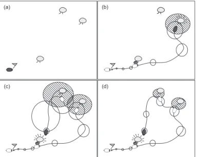
Since nothing can be observed from outside (should it be a landmark or the robot itself), uncertainties of measures get accumulated every time step. The more the mission lasts, the more the robot gets lost. Likewise, detection of landmarks is achieved with less and less accuracy. However, when the robot detects again a landmark that was already placed with a good accuracy on the map, its position can be adjusted from that of the landmark and the whole process of estimation (trajectory and map building) can be refined (see Figure 1). Hence, localization
(b)
(d) (c)
(a)
Fig. 1: A simple SLAM example. The robot is a mouse and landmarks are trees. Un-certainties on the robot position (resp. trees) are represented by blank (resp. hatched) ellipsis. (a) At initial time, the robot knows where it is. (b) The uncertainty on the robot position increases while it moves. When a second tree is detected, there is a significant uncertainty on its real position. (c) The first tree is met again and used to adjust the position of the robot. (d) With a backward computation of the trajectory, uncertainties on the previous positions and observations are reduced.
and map building are two connected goals. This interdependence is one of the reason that makes traditional probabilistic approaches inadequate. In contrast, it makes no difficulty in the constraint programming framework, as shown below.
2.2 Basic Constraint Model
Let us now focus on a basic modeling of the SLAM. Many details on a real experiment (description of the robot, experimental setup, full constraint model, etc.) can be found in [7] and [8] that deal with SLAM in a submarine context.
The SLAM problem is cast into a CSP as follows. First, the motion of the autonomous robot obeys a differential equation: p′(t) = f (u(t)), where p(t) is
the position of the robot in space, u(t) a vector of m inputs (speed, rotation angles, etc.) and f a mapping from Rm
to R3. This equation can be cast into a CSP using a classical interval variant of the Euler method. Details can be found in [7] and [8]. The discretization introduces a set of (N + 1) variables p(0),. . .,
p(N )where δtis the time lapse between to measures and N δtthe total duration
of the mission. These variables represent a discretization of the trajectory p, i.e., ∀i, 0 ≤ i ≤ N, p(i)= p(t0+ iδt) (1)
has to be fulfilled. The discretization also introduces N constraints.
Thus, the CSP provides a rigorous enclosure of the trajectory, i.e., for every possible input u(t) there exists a feasible tuple (p(0), . . . , p(N )) such that the
trajectory p corresponding to the inputs satisfies (1). 2.3 Introducing Detections
Now that the motion of the vehicle has been cast into a CSP, let us take into account detections. In the mission, n landmarks have to be localized. Their coordinates will be denoted by o(1), . . . , o(n). Once the mission is over, a human
operator scans the waterfall of images provided by exteroceptive sensors. When a group of pixels are suspected to correspond to a landmark, a box encompassing the corresponding area is entered as a potential detection. The position of a pixel on the image can be directly translated into a distance between the landmark and the robot. First, the detection time τ (i) (i.e., the number of time steps since t0)
and the distance riare determined. Then, the landmark number σ(i) is identified
which amount to match detections with each others. Finally, a distance constraint dist(p(τ (i)), o(σ(i))) = ri between the landmark and the robot is added into the model. Therefore, in [7], the model was augmented as follows:
(P′) additional variables: o(1)∈ [o(1)], . . . , o(n)∈ [o(n)] domains: [o(1)] := (−∞, +∞), . . . , [o(n)] := (−∞, +∞) additional constraints:
dist(p(τ (i)), o(σ(i))) = ri (i = 1..k)
Humans are subject to three types of mistakes: (1) Omission, a landmark on the waterfall is missed by the operator; (2) Illusion, the operator adds a detec-tion where there is no landmark; (3) Mismatching, the operator makes a wrong identification (do not match detections properly). On the one hand, the two first types of mistakes have been experimentally proven as irrelevant1. On the other 1 The overall accuracy may suffer from a lack of detections but the consistency of the
model is always maintained (at any time, many landmarks are anyway out of the scope of the sensors and somehow “missed”). Besides, perception is based on very specific visual patterns that rule out any confusion with elements of the environment.
hand, if identifying the type of a landmark is fairly easy, recognizing one partic-ular landmarkis very hard. In other words, the main difficulty in the operator’s task is matching landmarks with each others. The bad news is that mismatch-ing makes the model inconsistent. Hence, the third type of mistakes is critical and requires a lot of energy to be avoided. Up to now, in the experiments made in [7, 8], matching was simply performed using a priori knowledge of seamark positions.
2.4 Our contribution
The ambition of our work is simply to skip the operator’s matching phase. The idea is to use the knowledge on the number of landmarks to make this matching automatically by propagation. This is a realistic approach. In all the missions performed with submarine robots, a set of beacons is dropped into the sea to make the SLAM possible. The positions of the beacons at the bottom is not known because of currents inside water (consider also that in hostile areas they may be dropped by plane) but their cardinality is.
3
The Number of Distinct Vectors Constraint
Consider k vectors of variables x(1), . . . , x(k) of equal dimension (which is 2
or 3 in practice) and an integer-valued variable n. The constraint nvector(n, {x(1), . . . , x(k)}) holds if there is n distinct vectors between x(1) and x(k)which
can be written:
nvector(n, {x(1), . . . , x(k)}) ⇐⇒ |{x(1), . . . , x(k)}| = n,
where |{x(1), . . . , x(k)}| stands for the cardinality of the set of “values” taken
by x(1), . . . , x(k). An equivalent definition that better conform to the intuition
behind is that the number of distinct “values” in {x(1), . . . , x(k)} equals to n.
A family of constraints can be derived from nvector in the same way as for nvalue[2]. The constraint more specifically considered in this paper is atmost nvectorthat bounds the number of distinct vectors:
atmost nvector(n, {x(1), . . . , x(k)}) ⇐⇒ |{x(1), . . . , x(k)}| ≤ n. It must be pointed out that, with continuous domains, the constraints nvector and atmost nvector are operationally equivalent. Indeed, excepted in very par-ticular situations where some domains are degenerated intervals (reduced to sin-gle points), variables can always take an infinity of possible values. This means that any set of k non-degenerated boxes always share at least n values. In the nvector constraint, only the upper bound (“at most n”) can actually filters. This remark generalizes the fact that all diff is always satisfied with non-degenerated intervals. Figure 2a shows an example with n = 2 (the variable is ground) and k = 5 in two dimensions. Figure 2b shows the corresponding result of a bound consistency filtering.
000000000 000000000 000000000 000000000 000000000 000000000 000000000 111111111 111111111 111111111 111111111 111111111 111111111 111111111 0000 0000 0000 0000 0000 0000 0000 0000 0000 0000 0000 0000 0000 0000 0000 0000 0000 0000 0000 1111 1111 1111 1111 1111 1111 1111 1111 1111 1111 1111 1111 1111 1111 1111 1111 1111 1111 1111 [x(3)] [x(5)] [x(4)] v(1) v(2) [x(1)] [x(2)]
(a) Initial state
000000000 000000000 000000000 000000000 000000000 000000000 000000000 000000000 111111111 111111111 111111111 111111111 111111111 111111111 111111111 111111111 0000 0000 0000 0000 0000 0000 0000 0000 0000 0000 0000 0000 0000 0000 0000 0000 0000 0000 0000 1111 1111 1111 1111 1111 1111 1111 1111 1111 1111 1111 1111 1111 1111 1111 1111 1111 1111 1111 [x(4)] [x(2)] [x(3)] [x(5)] [x(1)] (b) Final state
Fig. 2: (a) The atmost nvector constraint with n = 2 and k = 5. The domains of x(i)is the cross product of two intervals [x(i)] = [x(i)
1 ] × [x (i)
2 ]. The constraint is satisfiable
be-cause there exists two vectors v(1)and v(2)such that ∀i, 1 ≤ i ≤ n, [x(i)]∩{v(1), v(2)} 6=
∅. The set of all such pairs (v(1), v(2)) is represented by the two little dashed boxes. (b) Result of the bound consistency with respect to the atmost nvector constraint. The domain of [x(4)] encloses the two little rectangles.
4
Operational Complexity
Enforcing generalized arc consistency (GAC) for the atmost-nvalue constraint is NP-hard [3]. Worse, simply computing the minimum number of distinct val-ues in a set of domains is NP-hard [2]. However, when domains are intervals, these problems are polynomial [1, 6]. The question under interest is to know if atmost-nvectoris still a tractable problem when domains are boxes (vector of intervals), i.e., when the dimension is greater than 1. We will show that it is not. Focusing on this type of domains is justified because continuous constraints are always handled with intervals. This also implies that bound consistency is the only acceptable form of filtering that can be applied with continuous domains.2
We shall restrict ourselves to the calculation of the minimum number of distinct values (also called the minimum cardinality) and to boxes of dimension 2, i.e., rectangles. As noticed in [2], the minimum number of distinct values shared by a set of rectangles is also the cardinality of the minimum hitting set. A hitting set is a collection of points that intersects each rectangle. In the two following subsections, we consider the equivalent problem of finding the cardinality of the minimum clique partitionof a rectangle graph.
4.1 Rectangle Graphs and Clique Partitions
A rectangle graph is a n-vertices graph Gr = (Vr, Er) that can be extracted
from n axis-aligned rectangles in the plane by (1) creating a vertex for each
2 Allowing gaps inside intervals and applying GAC filtering leads to unacceptable
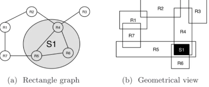
a rectangle, and (2) adding an edge when there is a non-empty intersection between two rectangles. Figure 3 depicts the two views of a rectangle graph. A clique partition of a graph is a collection of complete subgraphs that parti-tion all the vertices. A minimal clique partiparti-tion is a clique partiparti-tion with the smallest cardinality (i.e., with the smallest number of subgraphs). Since any set of pairwise intersecting rectangles intersect all mutually (by Helly’s theorem), a k-clique in a rectangle graph represents the intersection of k rectangles in the geometrical view. For instance, the 3-clique S1 of Gr in Figure 3a represents
the intersection of three rectangles (R4, R5, R6) in Figure 3b, depicted by the black rectangle S1. As a consequence, looking for the minimum hitting set or the
S1 R1 R2 R4 R3 R7 R5 R6
(a) Rectangle graph
R1 R7 R5 R4 R2 R3 R6 S1 (b) Geometrical view
Fig. 3: A rectangle graph and its geometrical representation (axis-aligned rectangles).
minimum clique partition are indeed equivalent problems for rectangle graphs. The final problem under consideration can then be formulated as follows:
Rectangle Clique Partition (RCP)
– Instance: A rectangle graph Gr = (Vr, Er) given in the form of |Vr|
axis-aligned rectangles in the plane and k ≤ |Vr|.
– Question: Can Vr be partition into k disjoint sets V1, . . . , Vk such that
∀i, 1 ≤ i ≤ k the subgraph induced by Vi is a complete graph?
Proposition 1. RCP is NP-complete.
The fact that RCP belongs to NP is easy to prove: the given of a k–partition is a certificate that can be checked in polynomial time. The rest of the proof, i.e., the reduction of a NP-complete problem to RCP is given below. Note that the transformation below is inspired from that in [10] but contains fundamental differences.
4.2 Building a Rectangle Graph from a Cubic Planar Graph
The problem we will reduce to RCP involves planar graphs which require the introduction of extra vocabulary. An embedding of a graph G on the plane is a
representation of G (see Figure 4) in which points are associated to vertices and arcs are associated to edges in such a way:
– the endpoints of the arc associated to an edge e are the points associated to the end vertices of e,
– no arcs include points associated to other vertices,
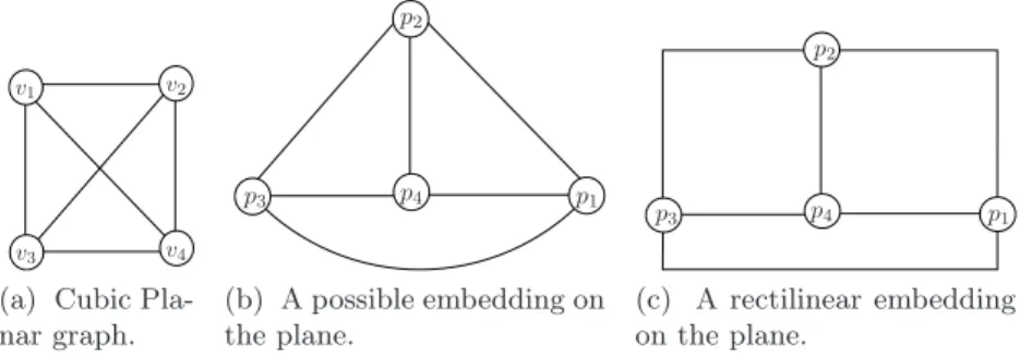
– two arcs never intersect at a point which is interior to either of the arcs. A planar graph (Figure 4a) is a graph which admits an embedding on the plane (Figure 4b), and a cubic graph is a 3-regular graph, i.e., a graph in which every vertex has 3 incident edges. A rectilinear embedding is an embedding where every arc is a broken line formed by horizontal and vertical segments (Figure 4c).
v1
v3
v2
v4 (a) Cubic Pla-nar graph. p1 p4 p2 p3 (b) A possible embedding on the plane. p3 p2 p1 p4 (c) A rectilinear embedding on the plane.
Fig. 4: A (cubic) planar graph, one of its embedding on the plane, and one of its rectilinear embedding.
We are now in position to discuss about the transformation itself. Consider a pla-nar cubic graph GP. First, Tammassia and al. gave a polytime algorithm in [11]
for computing a 5-rectilinear embedding of a planar graph, i.e., a rectilinear embedding where each broken line is formed by 5 segments. This is illustrated by Figure 5. Second, this embedding can be transformed into a rectangle graph
p3 p4 p1
p2
Fig. 5: A 5-rectilinear embedding of the cubic planar graph given in Figure 4 (segments are delineated by arrows).
using the patterns depicted on Figures 6a and 6b:
– Every segment of the 5-rectilinear embedding of Gpis replaced by a rectangle
such that if two segments do not intersect in the 5-rectilinear embedding, the corresponding rectangles do not intersect (should they be flat).
– For segments having a vertex at a common endpoint, the corresponding rectangles intersect all mutually in the neighborhood of this vertex (Figure 6a). Remember that the case of a leaf node is irrelevant because Gpis cubic.
– For segments having a bend in common, the rectangles are disjoint.
– An extra rectangle is added in the neighborhood of each bend. This rectangle intersects the two rectangles associated to the segments (Figure 6b). The three rectangles cannot intersect all mutually due to the previous point.
p S R3 R2 R1 R1 R2 R3
(a) Transformation of segments at a common endpoint.
R1 R2
R3
R3 R1 R2
(b) Transformation of segments having a bend in common.
Fig. 6: Atomic operations to transform the 5-rectilinear embedding of a cubic planar graph (left) into the geometrical view (middle) of a rectangle graph (right).
4.3 Reduction From Cubic Planar Vertex Cover
Consider the well-known vertex cover problem. This problem remains NP-Complete even for cubic planar graphs [12]. It is formally stated as follows:
Cubic Planar Vertex Cover (CPVC)
– Instance: A cubic planar graph Gp= (Vp, Ep) and k ≤ |Vp|.
– Question: Is there a subset V′ ⊆ V
pwith |V′| ≤ k such each edge of Ephas
at least one of its extremity in V′?
Lemma 1. Let Gp be a n-vertex m-edges cubic planar graph and an integer
value k≤ n. Let Grbe the rectangle graph obtained by the transformation of§4.2.
The answer to CPVC with (Gp, k) is yes iff the answer to RCP with (Gr, k+
4 × m) is yes.
Proof. This proof is illustrated in Figure 7.
Forward implication:Assume a n-vertex m-edges cubic planar graph Gp has
a vertex cover V′ of cardinality k. We shall build a partition P of G
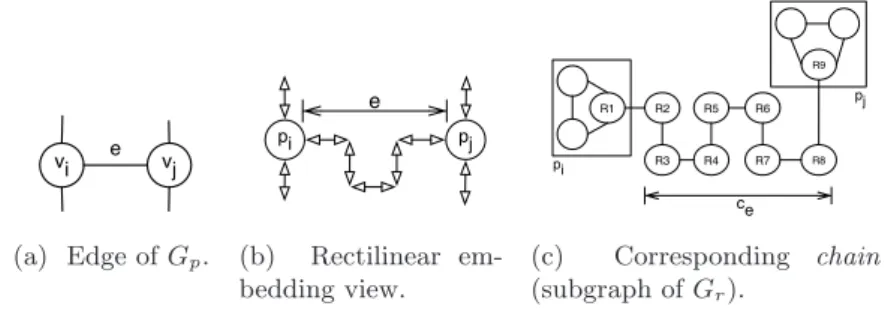
empty. To each edge e = (vi, vj) of Ep corresponds a 2-degree chain ce in Gr,
with exactly nine vertices, from a vertex of the 3-clique pi(associated to vi) to a
vertex of the 3-clique pj (associated to vj).
First, for every vi ∈ V′, add the 3-clique pi in P. Since V′ is a covering set,
every chain has now one of its extreme vertex inside a clique of P. The 8 other remaining vertices of the chain can then easily be partitioned into 4 additional cliques. Add these cliques to P.
Once all these additional cliques are added to P, the latter is a partition of Gr
whose size is k + 4 × m. vi e vj (a) Edge of Gp. pj pi e (b) Rectilinear em-bedding view. R1 R2 R3 R4 R5 R6 R7 R8 R9 pi pj ce (c) Corresponding chain (subgraph of Gr).
Fig. 7: Transforming an edge of the cubic planar graph GP into, first, its rectilinear
view, second, a rectangle graph Gr.
Backward implication:Assume Grcan be partition into k + 4 × m cliques and
let P be such a partition. We shall call a free clique a clique that only contain vertices of the same given chain. Similarly, a shared clique is a clique involving (extreme) vertices of at least two different chains.
Every chain contains 9 vertices. One can easily see that it requires at least 5 cliques to be partitioned, 4 of which are free. For every chain c, remove 4 free cliques of c from P. Then there is still (at least) one clique left in P that involves a vertex of c. When this process is done, the number of remaining cliques in P is k + 4 × m − 4 × m = k.
Now, for every clique C of P: if C is shared, put the corresponding vertex of GP in V′. If C is free, consider the edge e of GP associated to the chain and
put anyone of the two endpoint vertices of e into V′. We have |V′| = k and
since every chain has a vertex in the remaining cliques of P, every edge of GP
is covered by V′. ⊓⊔
5
A Very First Polytime Contractor
We shall now propose a simple algorithm for computing bound consistency with respect to atmost nvector. Let us denote by dim the dimension of the vectors.
The contractor is derived from the following implication: atmost nvector(n, {x(1), . . . , x(k)}) =⇒ atmost nvalue(n, {x(1) 1 , . . . , x (k) 1 }) ∧ . . . ∧ atmost nvalue(n, {x (1) dim, . . . , x (k) dim}).
Therefore, applying a contractor for atmost nvalue with the projections of the boxes onto each dimension in turn gives a contractor for atmost nvector. Since a contractor for atmost nvalue enforcing GAC (hence, bound consistency) when domains are intervals already exists [1], we are done. This is achieved in O(dim× klog(k)). Although the purpose of this paper is not to describe an efficient contractor, we shall introduce right away a first (but significant) improvement of our naive algorithm.
000000000000000 000000000000000 000000000000000 000000000000000 000000000000000 000000000000000 111111111111111 111111111111111 111111111111111 111111111111111 111111111111111 111111111111111 000000000000 000000000000 000000000000 000000000000 000000000000 000000000000 000000000000 111111111111 111111111111 111111111111 111111111111 111111111111 111111111111 111111111111 projection onto kernels [x(5)] [x(6)] [x(7)] [x(2)] [x(1)] [x(3)] [x(1)1 ] [x(5)1 ] [x(4)1 ] [x(3)1 ] [x(7)1 ] [G1] [G2] x1 [G3] [x(4)] [x(2)1 ] [x(6)1 ]
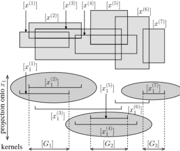
Fig. 8: Illustration of what the at most nvalue algorithm yields. Here, k = 7, dim = 2, n= 3 and the algorithm is run for the first projection (i.e., onto the horizontal axis). Three groups, represented by gray ellipsis, are identified, namely G1 = {x(1)1 , x
(2) 1 },
G2= {x(4)1 , x (5)
1 } and G3= {x(7)1 }. The variables of the same group are proven to be all
equal (otherwise, the constraint is violated). E.g., x(1)1 and x(2)1 must satisfy x(1)1 = x(2)1 . Domains for the variables of a given group can be replaced by the corresponding kernel (e.g., [x(1)1 ] and [x(2)1 ] can be set to [G1]). Notice that the kernels are all disjoint.
In our suggested improvement, the whole boxes are intersected instead of the first components only. Hence the domains of [x(1)] and [x(2)] are intersected, which gives
one of the hatched rectangles. The other hatched rectangle is [x(4)] ∩ [x(5)].
The reader must simply admit that the contractor of atmost nvalue(n, {x(1)i ,
. . ., x(k)i }) works in two steps (see Figure 8). First, it builds groups of variables.
If the number of groups turns to be n, it is then proven that for all x(j)i and
x(l)i that belong to the same group, x(j)i and x(l)i must satisfy x(j)i = x(l)i . Hence, the domains of all the variables of the same group G can be shrunk to their
common intersection denoted by [G]. Furthermore, this process results in a set of n disjoint intervals [G1], . . . , [Gn] that we will call kernels.
In the favorable case of n groups, the last step can be improved. If two variables x(j)i and x(l)i belong to the same group G, the whole vector variables x
(j)and x(l)
are actually constrained to be equal. Indeed, assume that x(j)and x(l)could take
two different vectors. The k − 2 other variables necessarily share n − 1 different vectors because their ithcomponents must “hit” the n − 1 (disjoint) kernels [G′]
with G′ 6= G. This means that the overall number of distinct vectors is at least
(n − 1) + 2 > n.
Hence, the algorithm of atmost nvalue can be modified to intersect boxes (in-stead of just one component). This multiplies the complexity by dim (which is small in practice).
6
Experimental Evaluation: the SLAM Problem
This section shows how the atmost nvector constraint allows to improve the modeling and resolution of the SLAM problem. We propose an extension of the original model given in Section 2, and provide a graphical validation.
We introduce k 3-dimensional variables d(1), . . . , d(k) related to all the
detec-tions. A distance constraint involving each of the latters is added into the model, as well as a nvector constraint capturing the fact that only n landmarks exist.
(P′′) additional variables: d(1)∈ [d(1)], . . . , d(k)∈ [d(k)] domains: [d(1)] := (−∞, +∞), . . . , [d(k)] := (−∞, +∞) additional constraints:
dist(pτ(i), d(i)) = ri (i = 1..k) atmost− nvector(n, {d(1), . . . , d(k)})
The introduction of the atmost-nvector constraint has provided the expected results. Let us first explain how the benefits of this constraint can be quantified. In the context of differential equations, we are dealing with a very large number of variables and a sparse system with an identified structure. Moreover, the system is subject to many uncertainties. Under these conditions, the quality of the result is more relevant than the computation time, as we justify now.
No choice point. In applications, the number of variables can be huge (more than 1140000 in [7, 8] in order to represent the three coordinates of the robot, the Euler angles, the speed, the altitude and the components of the rotation matrix at each time step). This prevents us for making choice points. Note that the situation is even worse since the solution set is not a thin trajectory (formed by isolated points). The numerous uncertainties make the best solution ever a thick
beam of trajectories (as depicted in Figure 9). Continuums of solutions usually dissuade one from making choice points, even for much smaller problems. Handcrafted propagation. The size of our problem also prevents us for using a general-purpose AC3-like propagation algorithm, since building an adjacency matrix for instance would simply require too much memory. Furthermore, we have a precise knowledge of how the network of constraints is structured. Indeed, the discretization of the motion yields a single (long) chain of constraints and cycles in the network only appear with detection constraints. An appropriate strategy is then to base propagation on the detection constraints, which are much fewer. Every time a detection reduces significantly the domain of a position p(i),
the motion constraints are propagated forward (from p(i)to p(N )) and backward
(from p(i) downto p(0)). In a nutshell, propagation in this kind of problems is
guided by the physics.
Irrelevance of computation time. When the application is run, it takes a couple of seconds to load data of the sensors (which amount to initialize the domains of variables representing input vectors) and to precalculate expressions (e.g., rotation matrices). With or without the nvector constraint, propagation takes a negligible time (less than 1%) in comparison to this initialization. There-fore, focusing on computation time is not very informative.
Quality of the result. Our contribution is to make propagation for the SLAM problem automatic whereas part of it was performed by a human operator so far. This is a result in itself. However, one may wonder which between the automatic matching and the operator’s is most competitive. This, of course, is hard to evaluate a priori. In the experiment of [7, 8], both have provided the optimal matching. The question that still remains is to know the extent to which our matching (the one provided by the algorithm in Section 5) improves the “quality” of the result, i.e., the accuracy of the trajectory.
The idea was to make the robot looping around the same initial point so that many detections would intersect.3For this purpose, we have controlled the robot
with a classical feedback loop which gives the expected cycloidal trajectory. Four landmarks have been placed in the environment and we have basically considered that a landmark is detected everytime the distance between the robot and itself reaches a local minimum (if less than a reasonable threshold). The estimation of the landmark position is then calculated from this distance (with an additional noise) and a very rough initial approximation.
Figure 9 illustrates the effect of automatic matching on the estimation of the trajectory and the positions of the landmarks. All the results have been obtained in a couple of seconds by the Quimper system [5].
3 The experiment of [7, 8] was not appropriate for this illustration because matching
seamarks was actually too easy (6 seamarks and a rectangle graph of detections with 6 strongly connected components).
(a) Basic SLAM: trajectory and de-tections (1200 iterations).
(b) Basic SLAM: Detections (4000 iterations).
(c) Basic SLAM: trajectory (4000 it-erations).
(d) Improved SLAM: trajectory and detections (4000 iterations).
Fig. 9: Comparing SLAM with the atmost-nvector contractor (Improved SLAM) and without(Basic SLAM). The trajectory is represented by gray filled boxes, detections by thick-border rectangles and landmarks by the little black squares. Figure 9(d) depicts the fixpoint of all the contractors: the four landmarks are very well localized and the trajectory is much thiner (after 4000 iterations, the largest diameter is 10 times less than in Figure 9(c)). Our algorithm has contracted many detections to optimal boxes around landmarks. We can also observe the weakness of our algorithm which has poorly reduced boxes whose projections on both axis encompass two projections of landmarks. This however exclude a detection which really encloses two landmarks: in this case, either there is a real ambiguity or it is the propagation to blame.
7
Conclusion
A somewhat natural generalization of the nvalue constraint, called nvector has been proposed. The nvector constraint can help modeling and solving many
localization problems where a bound on the number of landmarks to localized is known. This has been illustrated on the SLAM problem and applied on a real experiment. We have also analyzed the complexity of this global constraint and given a simple contractor.
The benefit of this constraint in terms of modeling has a direct impact on the way data of the experiments have to be processed. Indeed, the constraint allows to avoid requiring someone that matches landmarks by hand. Hence, it reduces considerably the amount of work and the probability of mistake this operation entails.
The field of application is not restricted to the SLAM problem. Ongoing works show that the nvector is as crucial for the passive location of vehicles using TDOA (time difference of arrival) in signal processing. All these problems involve real variables. Hence, as a side contribution, this paper also offsets the lack of activity about global continuous constraints.
Future works include the design of more sophisticated contractors with bench-marking. The nvector constraint also leads up to the study of other global constraints. As soon as several estimations of the same landmark position are matched by nvector, this position satisfies indeed a global constraint (namely, the intersection of several spheres if estimations result from distance equations).
References
1. N. Beldiceanu. Pruning for the minimum Constraint Family and for the number of distinct values Constraint Family. In CP, pages 211–224. Lecture Notes in Computer Science, 2001.
2. C. Bessi`ere, E. H´ebrard, B. Hnich, Z. Kiziltan, and T. Walsh. Filtering Algorithms for the NValue Constraint. In CPAIOR’05, pages 79–93. Springer, 2005.
3. C. Bessi`ere, E. H´ebrard, B. Hnich, and T. Walsh. The Complexity of Global Constraints. In AAAI’04, pages 112–117, 2004.
4. G. Chabert. Techniques d’Intervalles pour la R´esolution de Syst`emes d’ ´Equations. PhD Thesis, Universit de Nice-Sophia Antipolis, 2007.
5. G. Chabert and L. Jaulin. Contractor Programming. Artificial Intelligence, 173:1079–1100, 2009.
6. U.I. Gupta, D.T. Lee, and Y.T. Leung. Efficient Algorithms for Interval Graphs and Circular-Arc Graphs. Networks, 12:459–467, 1982.
7. L. Jaulin. Localization of an Underwater Robot using Interval Constraint Propa-gation. In CP. Springer, 2006.
8. L. Jaulin. A Nonlinear Set-membership Approach for the Localization and Map Building of an Underwater Robot using Interval Constraint Propagation. IEEE Transaction on Robotics, 25(1):88–98, 2009.
9. R. Moore. Interval Analysis. Prentice-Hall, 1966.
10. C.S. Rim and K. Nakajima. On Rectangle Intersection and Overlap Graphs. IEEE Transactions on Circuits and Systems, 42(9):549–553, 1995.
11. R. Tamassia and I.G. Tollis. Planar Grid Embedding in Linear Time. IEEE Trans. Circuits Systems, 36:1230–1234, 1989.
12. R. Uehara. NP-Complete Problems on a 3-connected Cubic Planar Graph and their Applications. Technical Report Technical Report TWCU-M-0004, Tokyo Woman’s Christian University, 1996.